Type-1 OWA Operators in Aggregating
Multiple Sources of Uncertain Information :
Properties and Real World Applications
Shang-Ming Zhou,
Member, IEEE,
Francisco Chiclana, Robert I. John,
Senior Member, IEEE,
Jonathan M. Garibaldi,
Senior Member, IEEE,
and Lin Huo
Abstract—The type-1 ordered weighted averaging (T1OWA) operator has demonstrated the capacity for directly aggregating multiple sources of linguistic information modelled by fuzzy sets rather than crisp values. Yager’s OWA operators possess the properties of idempotence, monotonicity, compensativeness, and commutativity. This paper aims to address whether or not T1OWA operators possess these properties when the inputs and associated weights are fuzzy sets instead of crisp numbers. To this end, a partially ordered relation of fuzzy sets is defined based on the fuzzy maximum (join) and fuzzy minimum (meet) operators of fuzzy sets, and an alpha-equivalently-ordered relation of groups of fuzzy sets is proposed. Moreover, as the extension of orness and andnessof an Yager’s OWA operator,joinnessand meetness of a T1OWA operator are formalised, respectively. Then, based on these concepts and the Representation Theorem of T1OWA operators, we prove that T1OWA operators hold the same properties as Yager’s OWA operators possess, i.e.: idempotence, monotonicity, compensativeness, and commutativity. Various numerical examples and a case study of diabetes diagnosis are provided to validate the theoretical analyses of these properties in aggregating multiple sources of uncertain information and improving integrated diagnosis, respectively.
Index Terms—OWA operator, type-1 OWA operator, ag-gregation, linguistic agag-gregation, fuzzy sets, soft decision making, diabetes, integrated diagnosis.
I. Introduction
In domains where information fusion/integration or multi-factorial evaluation is needed, an aggregation pro-cess is nepro-cessary to combine multiple sources of
infor-Manuscript received ***, 2018.(Corresponding author: Shang-Ming Zhou, Lin Huo)
This work is supported by the EPSRC Research Grant EP/C542215/1, Major Project of National Social Science Foundation of China (16ZDA0092), and Guangxi University ‘Digital ASEAN Cloud Big Data Security and Mining Technology’ Innovation Team.
Shang-Ming Zhou is with Health Data Research UK, Institute of Life Science, Swansea University, UK (E-mail: [email protected]; [email protected]).
Francisco Chiclana is with the the Institute of Artificial Intelligence, De Montfort University, Leicester, UK; the Dept. of Computer Science and Artificial Intelligence, University of Granada, Spain (E-mail: [email protected]).
Robert I. John and Jon M. Garibaldi are with School of Computer Science, University of Nottingham, Nottingham, UK (E-mail:[email protected]; [email protected]).
Lin Huo is with China-ASEAN Research Institute, Guangxi Univer-sity, Nanning, Guangxi, China (Email:[email protected]).
mation into a global result so that in the final deci-sion, all the individual sources of information are taken into account [1]. For example, in medicine, diagnosis or measurement can rarely be decided based on an individual criterion. Particularly, in the age of big data, the use of information aggregation is rapidly increas-ing, both because data is easily collected by ubiquitous information technologies and because the availability of cost-effective computational power allows combining information from multiple sources to be readily feasible. Yager’s ordered weighted averaging (OWA) operators [2], [3] have become a popular tool to aggregate infor-mation from multiple sources due to their flexibility for modeling a wide variety of aggregation scenarios via the appropriate definition/selection of the OWA operator’s weighting vector [3]. However, Yager’s OWA operators exclusively aggregate crisp numbers, while in real-world decisions, one is often not certain about the exact value of a crisp attribute. For example, in medicine, patients often find it difficult to describe how they feel, and doc-tors/nurses often find it difficult to describe what they observed. Thus it is desirable to develop a technique that can aggregate multiple sources of uncertain information of attributes. T1OWA operators and the associated α-level T1OWA aggregations are such a technique [4], [5], in which uncertain information is modelled by fuzzy sets. In this way, with appropriately definitions of un-certain weights, T1OWA operators extend Yager’s OWA operator [2], themeetoperator of fuzzy sets and thejoin
operators of fuzzy sets [7], [8].
Since their appearance, the T1OWA operators have received increasing attention in scientific applications [9]–[14]. To select optimal routes under uncertain en-vironments, T1OWA operators have been designed to guide human decision-making in a fuzzy weighted graph [10]. In addition to the α-level approach to fast imple-mentation of T1OWA operators, another new method of calculating T1OWA was proposed via an opposite direction searching [11]. A T1OWA unbalanced fuzzy linguistic aggregation method has been applied to credit risk evaluation [12]. In group decision making, T1OWA operators can be used to combine multiple granular linguistic information and improve consensus reaching processes [13]. In type-2 fuzzy logic system modelling, the type-reduction of general type-2 fuzzy sets can be
1 2 3 4 5 6 7 8 9 10 11 12 13 14 15 16 17 18 19 20 21 22 23 24 25 26 27 28 29 30 31 32 33 34 35 36 37 38 39 40 41 42 43 44 45 46 47 48 49 50 51 52 53 54 55 56 57 58 59 60
efficiently implemented via T1OWA operators [14]. Despite the above mentioned advances on the devel-opment and applications of T1OWA operators, one issue remains unclear regarding aggregation mechanism prop-erties. Yager’s OWA operators areidempotent,monotonic,
compensative, and commutative [2]. The question to be answered in our case is whether or not T1OWA oper-ators hold these same properties when the inputs and associated weights become uncertain, being expressed as fuzzy sets instead of crisp numbers in soft decision making. This question is not trivial at all, because the mechanisms of operations on a group of (fuzzy) sets are completely different from those on crisp values, with more advanced computing techniques to be required. In this paper, we aim to answer this important question.
To this end, based on the α-cuts of fuzzy sets, we suggest a new relation of fuzzy sets, named the alpha-equivalently-orderedrelation of a group of fuzzy sets, and address thejoinand themeetbasedpartial order relation
of fuzzy sets. Then we prove that the T1OWA operation is commutative, idempotent,monotonic, and compensative
with respect to the fuzzy set partial order relation. The rest of this paper proceeds as follows. In Sec-tion II, we briefly review two definiSec-tions of the T1OWA operator: one based on theExtension Principle, the other based on the α-cuts of fuzzy sets. Section III defines a fuzzy set partial order relation based on the meet and join operators of fuzzy sets. As the extension of the
andness andornessof Yager’s OWA operators. Section IV defines the meetness and joinness of T1OWA operators. The properties of a T1OWA operator are then analysed and proved in Section V. Section VI provides a case study of diabetes diagnosis and further validation of computing efficiency ofα-level T1OWA aggregation. The paper concludes with Section VII.
II. Preliminaries
Although the T1OWA operators can be defined either via Zadeh’s Extension Principle or via the α-cuts of fuzzy sets [4], [5], their final aggregation results coincide.
Let F(X) be the power set of fuzzy subsets on the domain of discourse X. One can define the T1OWA operator via the Extension Principle [4] as follows: Definition 1. “Given n linguistic weights nWfi
on
i=1 in the form of fuzzy sets defined on the domain of discourse U = [0,1], a T1OWA operator is a mappingΦ,
Φ:F(X)× · · · ×F(X) −→ F(X) (Ae1,· · ·,Aen) 7→ Ye
(1)
The membership function of outcome fuzzy set Ye
(aggrega-tion result) is µeY(y) = sup n X i=1 ¯ wiaσ(i)=y wi∈U , ai∈X µfW1(ω1) ∧ · · · ∧µ f Wn(ωn) ∧µ e A1(a1)∧ · · · ∧µAen(an) ! (2) where ω¯i= Pnωi i=1ωi, and σ: {1,· · ·, n} −→ {1,· · ·, n}is a
per-mutation function such thataσ(i)≥aσ(i+1), ∀i= 1,· · ·, n−1, i.e.,aσ(i) is the ith largest element in the set{a1,· · ·, an}.”
Definition (2) can lead to a procedure for implement-ing T1OWA operations, called the Direct Approach [4]. Alternatively, one can define T1OWA operators using the α-cuts of a fuzzy set [5] as follows:
Definition 2. “Let nWfi on
i=1 be a set of linguistic weights characterised by fuzzy sets on the domain of discourseU = [0,1], andα∈[0,1].Theα-level type-1 OWA operator with α-cutsnWfαi
on
i=1is the operator that aggregates theα-cuts of the fuzzy sets{Ae1,· · ·,Aen}as follows:
ΦαAe1α,· · ·,Aenα = n P i=1 ωiaσ(i) n P i=1 ωi ωi∈Wfαi, ai∈Aeiα, i= 1,· · ·, n (3)
where σ is a permutation function such that aσ(i) ≥
aσ(i+1),∀i= 1,· · ·, n−1, Wfαi ={ω|µ f Wi(ω)≥α}, and Aeiα = {x|µ e Ai(x)≥α}.”
In fact, one can use theα-level setsΦαAe1α,· · ·,Aenα
to create a fuzzy set as follows:
e G= ∪ 0≤α≤1αΦα e A1α,· · ·,Aenα (4) where the membership function is
µGe(x) = ∨
α:x∈Φα(Ae1α,···,Aenα)
α (5)
The above two methods of aggregating fuzzy sets via Yager’s OWA mechanism are equivalent [5] as stated below.
Theorem 1 (Representation Theorem of T1OWA Op-erators). “Given a set of linguistic weights nWfi
on
i=1 in the form of fuzzy sets on U. For any fuzzy sets Ae1,· · ·,Aen on F(X), letY be the outcome aggregation result defined in (2) and Gebe the result defined in (4), then Ye=Ge.”
According to this Representation Theorem, one can implement the T1OWA aggregation through a series of α-level T1OWA operators. This provides a new way of theoretically analysing the properties of T1OWA op-erators. The procedure for implementing the T1OWA aggregation through a series ofα-level T1OWA operators is called theAlpha-Level Approach[5].
III. Join and Meet Based Partial Order Relation of Fuzzy Sets
Zadeh defined the meet and the join of fuzzy sets to aggregate linguistic variablesAeandeBfor the statements “Aeand B” and “e Aeor B” respectively [6]. Thee meet and thejoinof fuzzy sets now become fundamental operators in developing type-2 fuzzy systems [7], [8].
1 2 3 4 5 6 7 8 9 10 11 12 13 14 15 16 17 18 19 20 21 22 23 24 25 26 27 28 29 30 31 32 33 34 35 36 37 38 39 40 41 42 43 44 45 46 47 48 49 50 51 52 53 54 55 56 57 58 59 60
Definition 3. Given two fuzzy sets eS and Te, the join (∪)
and meet (∩) operators are defined as µeS∪eT(v) = sup s∨t=v s, t∈X µeS(s) ∧µ e T(t) (6) µeS∩eT(v) = sup s∧t=v s, t∈X µeS(s) ∧µ e T(t) (7)
wheresupis a t-conorm,∧is the minimum operator and∨
is the maximum operator.
It should be noted that the join (6) and the meet (7) operators can aggregate a set of criteria based on an imperative, such as “one of the criteria should be satisfied” and “all the criteria should be satisfied” respectively [6].
A. Join and Meet are T1OWA Operators
By appropriately choosing linguistic weights in a T1OWA operator, the join operator (6) of fuzzy sets is, in fact, a special T1OWA operator.
Theorem 2. Let a T1OWA operator, J, be defined by the first linguistic weight being the singleton weight ˜1: Wf1= ˜1, all
other weights being the singleton weight ˜0: Wfi= ˜0 (i,1),
where, µ˜1(ω) = ( 1 f or ω= 1 0 f or ω,1 (8) µ˜0(ω) = ( 1 f or ω= 0 0 f or ω,0 (9) For any groups of fuzzy sets nAei
on i=1, JAe1,Ae2,· · ·,Aen =[n i=1Ae i (10) Proof. Omitted
Example 2in the Supplemental Materialshows thejoin
operation as a T1OWA operator in nature.
Interestingly, in T1OWA aggregation, if the first lin-guistic weight moves towards ˜1, all the others towards ˜0 (seeExample 3in theSupplemental Material), then this operator demonstrates a join-like behavior. This type of operator is called ajoin-likeT1OWA operator.
Similarly, the meet operation (7) of fuzzy sets is also a special T1OWA operator.
Theorem 3. Let a T1OWA operator, M, be defined by the last linguistic weight being the singleton weight ˜1 :Wfn= ˜1,
all the others being the singleton weight ˜0 :Wfi= ˜0 (i,n).
For any groups of fuzzy sets nAei on i=1, MAe1,Ae2,· · ·,Aen =\n i=1Ae i (11) Proof. Omitted
Example 5 in the Supplemental Material shows the results of the Meet operator to aggregate three fuzzy aggregated objects.
Correspondingly, in T1OWA aggregation, if the last linguistic weight moves towards ˜1, all the other weights
towards ˜0, then this operator demonstratesmeet-liketype behavior (seeExample 6in theSupplemental Material). We call it ameet-like T1OWA operator.
B. Partial Order Relation of Fuzzy Sets
The set of real numbersRis linearly ordered, and the (R,∧,∨) forms a lattice. Then, for anya, b∈R, a partially ordered relation “≥”(“≤”) can be defined as
s≥t ⇐⇒ s∨t=s
⇐⇒ s∧t=t (12)
As a matter of fact, according to Zadeh’ Extension Principle, the meet (∩) and join (∪) operators are just fuzzification of the min (∧ ) and max (∨) operators of crisp numbers, respectively. In this way,Se∩TeandSe∪Te are no other than the fuzzified minimum,S, and fuzzfiede maximum, Te, of the fuzzy sets. It can be proved that (F(R),∩,∪) is a distributive lattice [15], with partial order relation defined as follows:
Definition 4. Given two fuzzy numbers eS and Te, a
par-tially ordered relation“<” is defined as e
S<Te ⇐⇒ Se∪Te=Se ⇐⇒ Se∩Te=Te
(13) We have the following theorem:
Theorem 4. Let eS and Te∈F(R) be fuzzy numbers with
core centresv1 and v2 respectively, andv1≥v2, then based on the t-conorm and t-norm,
e S<Te ⇐⇒ µ e S(s)≤µTe(s)for s ≤v2 andµ e S(s)≥µeT(s) for s≥v1.
Proof. 1) First, ifeS<Te, then according to (13), for any s≤v2, we haveµ e T(v2) = 1 and µTe(s) =µeS∩eT(s) = sup s1∧s2=s s1, s2∈X µeS(s1) ∧µ e T(s2) Becausex∧v2=s, µTe(s) ≥µ e S(s)∧µTe(v2) =µeS(s)∧1 =µeS(s) For anys≥v1, we haveµ
e S(v1) = 1 and µeS(s) =µSe∪Te(s) = sup s1∨s2=s s1, s2∈X µeS(s1) ∧µ e T(s2) Becausev1∨s=s, µSe(s) ≥µ e S(v1)∧µeT(s) = 1∧µ e T(s) =µTe(s) 2) If µeS(s) ≤µ e
T(s) for any x≤v2 and µSe(s)
≥µ
e
T(s) for anys≥v1, we proveeS∪Te=eS in the following.
1 2 3 4 5 6 7 8 9 10 11 12 13 14 15 16 17 18 19 20 21 22 23 24 25 26 27 28 29 30 31 32 33 34 35 36 37 38 39 40 41 42 43 44 45 46 47 48 49 50 51 52 53 54 55 56 57 58 59 60
Let us denote Ce≡eS∪Te. For any s, s1 and s2 ∈X with s1 ∧s2 = s, then s = s1 or s = s2. Hence,
the membership function of fuzzy set Ce can be decomposed as follows: µCe(s) =u1(s) ∨u2(s) where u1(s) =s ∨ 1:s1≤s µeS(s1) ∧µ e T(s) =µTe(s) ∧ ∨ s1:s1≤s µeS(s1) ! u2(s) = ∨ s1:s1≤s µeS(s)∧µ e T(s1) =µeS(s) ∧ ∨ s1:s1≤s µTe(s1) ! Then if s ≤ v2, the µ e S(·) and µTe(
·) are both non-decreasing functions. So we have u1(s) = µeT(s)
∧ µeS(s), andu2(s) =µeS(s) ∧µ e T(s), which lead to µCe(s) =µeS(s) ∧µ e T(s) =µeS(s) If v2 ≤s≤v1, µeT( ·) is non-increasing, and µ e S(·) is non-decreasing. Then we have u1(s) =µTe(s)
∧µ e S(s), and u2(s) =µeS(s) ∧1 =µ e S(s), which lead to µCe(s) =µeS(s) ∨µ e T(s)∧µeS(s) =µeS(s) If v1 ≤ x, µTe( ·) is non-increasing, and µ e S(·) is non-increasing. So we have sup
s1:s1≤s µeS(s) = 1, and sup s1:s1≤x µTe(s) = 1. Then, µCe(s) =µeS(s) ∨µ e T(s) =µeS(s) HenceSe∪Te=eS.
Theorem 4 provides a more strict finding than that investigated by Ramik and Rimanex [15] in the context of fuzzification of the min and max operators, which states that Se < Te ⇐⇒ there must be v1, u∗ and v2
with v1 ≥u∗ ≥v2, µSe(v1) =µTe(v2) = 1, µeS(s)≤µeT(s) for
anys < u∗ andµeS(s)≥µTe(s) for any s > u∗.
Based on the α-cuts of fuzzy sets, the following order relation has been defined [15]:
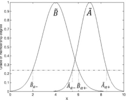
Definition 5. “For any fuzzy numberseSandTe, an ordering
relation e≥is defined as e Se≥Te ⇐⇒ Seα+≥Teα+andeSα−≥Teα−∀α∈[0,1] whereSeα= h e Sα−,Seα+ i andTα= h e Tα−,Teα+ i
are theα-cuts of
e
S and Te, respectively. ”
The following example shows an ordering relation between two fuzzy sets.
Example 1 (Ordering Relation). Figure 1 illustrates two fuzzy sets such that Aee≥Be.
Fig. 1: Two fuzzy setsAeandeBhaving ordering relation.
The relatione≥is a partially ordered relation onF(R), known as the fuzzy max order [15]. Interestingly, the two apparently different order relations , < and e≥, are equivalent onF(R) as it was proved in [15]:
Lemma 1. The following three relations are equivalent for any fuzzy numbersSeandTe:
i)See≥Te; ii)Se∪Te=Se; iii)Se∩Te=Te
IV. Joinness and meetness of a T1OWA operator A popular way to evaluate the behaviour of an OWA operator is to use the measure of orness and its dual
andness proposed by Yager [2], [3]. The two measures aim to assess the similarity of an OWA operator with the maximum and minimum operators, respectively based on the associated weighting vector.
Similarly, in T1OWA aggregation, the following def-initions of joinness and meetness associated with the linguistic weights evaluate how the T1OWA aggregation behaves like the operations ofjoinandmeet, respectively. Definition 6. For a T1OWA operator with fuzzy set weights
n f Wi
on
i=1on U⊆[0, 1], its joinness is:
µjoinness(u) = sup jω1,···,ωn=u
µWf1(ω1)
∗ · · · ∗µ
f
Wn(ωn) (14)
where∗is a t-norm operator, and jω1,···,ωn= 1 (n−1)Pn i=1 ωi n X i=1 (n−i)ωi (15)
The corresponding meetness of the T1OWA is:
µmeetness(u) = sup mω1,···,ωn=u µWf1(ω1) ∗ · · · ∗µ f Wn(ωn) (16) where mω1,···,ωn= 1− 1 (n−1)Pn i=1 ωi n X i=1 (n−i)ωi (17)
Clearly, the definedjoinnessandmeetnessof a T1OWA are fuzzy sets describing the linguistic expressions of ag-gregations behaving like thejoin andmeet, respectively.
1 2 3 4 5 6 7 8 9 10 11 12 13 14 15 16 17 18 19 20 21 22 23 24 25 26 27 28 29 30 31 32 33 34 35 36 37 38 39 40 41 42 43 44 45 46 47 48 49 50 51 52 53 54 55 56 57 58 59 60
It is not difficult to calculate that the joinness and
meetness of the join operator as a particular T1OWA operator (see the Theorem 2), are joinnessnWfi
on i=1 = ˜1 and meetnessnWfi on i=1
= ˜0,which further confirms that this particular T1OWA operator is the join operator of fuzzy sets. Correspondingly, the joinness and meetness
of the meet operator as a particular T1OWA operator (see the Theorem 3), are joinnessnWfi
on i=1 = ˜0 and meetnessnWfi on i=1
= ˜1, confirming that this particular T1OWA operator is themeet operator of fuzzy sets.
Moreover, Example 4 in the Supplemental Material
depicts the joinness of the T1OWA operator shown in
Example 3 in theSupplemental Material. V. Properties of T1OWA Operators
Yager’s OWA operators possess the properties of idempo-tence, monotonicity, compensativeness, and commutativity
[2]. In this section, we investigate the conditions for these properties to be verified by T1OWA operators.
Firstly, because Yager’s OWA operators and the sup
operators in the (6) and (7) are commutative, the T1OWA operator iscommutativeas well according to its definition in (2).
Theorem 5. For any T1OWA operator Φ andAe1,· · ·,Aen∈ F(R),
ΦAe1,· · ·,Aen
=ΦAep1,· · ·,Aepn
where the sequence {p1,· · ·, pn} is a permutation of the
sequence {1,· · ·, n}.
The T1OWA operators with linguistic weights also verify the property of idempotence as addressed by the following Theorem.
Theorem 6. For any fuzzy numberAe, the T1OWA operators Φ with fuzzy number weights verify
ΦA,e· · ·,Ae
=Ae
Proof. Let y ∈R and w1,· · ·, wn, a1,· · ·, an ∈R such that y= Pn i=1 ¯ wiaσ(i) with ¯wi=wi n P i=1 wi.Convexity ofAe∈F(R) implies that µAe(y) =µAe n P i=1 ¯ wiaσ(i) ! ≥µ e A(aσ(1))∧ · · · ∧µAe(aσ(n)) =µAe(a1) ∧ · · · ∧µ e A(an) ≥µ f W1(w1)∧ · · · ∧µWfn(wn) ∧µ e A(a1)∧ · · · ∧µAe(an)
The above inequality is true for any possible set of values w1,· · ·, wn, a1,· · ·, an ∈ R such that y = n P i=1 ¯ wiaσ(i) and
therefore it is true that µAe(y)≥ sup n X k=1 ¯ wiaσ(i)=y wi∈U , ai∈R µWf1(w1)∧ · · · ∧µWfn(wn) ∗µ e A1(a1)∧ · · · ∧µAen(an) ! =µYe(y) whereYe=Φ e A1,· · ·,Aen .
In order to prove µYe(y) =µAe(y), we only need to find a specific combination of ˆw1,· · ·,wˆn, ˆa1,· · ·,aˆn∈R such thatµfW1( ˆw1) ∧ · · · ∧µ f Wn( ˆwn)∧µAe( ˆa1) ∧ · · · ∧µ e A( ˆan) reaches µAe(y). For fW
i (∀i) being a fuzzy number, there exists at least one value ˆwi such that µWfi( ˆwi) = 1 (
∀i). Taking ˆ ai=y (∀i), we have µWf1( ˆw1) ∧ · · · ∧µ f Wn( ˆwn)∧µA( ˆa1)∧ · · · ∧µAe( ˆan) =µAe(y)∧ · · · ∧µ e A(y) =µAe(y)
Consequently µGe(y) =µAe(y).
In what follows, we investigate how monotonicity is verified by T1OWA operators. Firstly, we propose the
alpha-equivalently-ordered relation between two sets of fuzzy numbers: Definition 7. LetnAei on i=1 and n e Bion
i=1 be two sets of fuzzy numbers. The σ and η represent permutations of{1,· · ·, n}
defined by nAeiα+ on i=1 and n e Aiα− on
i=1, respectively. If for any
α∈[0,1] e Aσα(1)+ ≥Ae σ(2) α+ ≥ · · · ≥Ae σ(n) α+ =⇒ e Bσα(1)+ ≥Be σ(2) α+ ≥ · · · ≥Be σ(n) α+ and e Aηα(1)− ≥Ae η(2) α− ≥ · · · ≥Ae η(n) α− =⇒ e Bηα(1)− ≥Be η(2) α− ≥ · · · ≥Be η(n) α−
then the fuzzy setsnBei on
i=1are said to be alpha-equivalently-ordered with the setsnAei
on i=1.
The following example illustrates the
alpha-equivalently-ordered relation, while Example 7 in theSupplemental Materialgives a counterexample of the
alpha-equivalently-ordered relation.
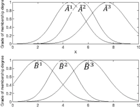
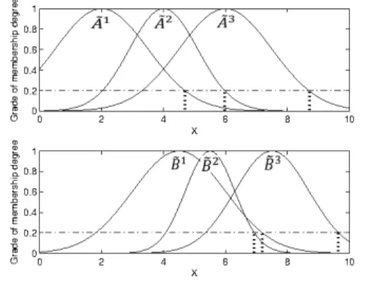
Example 2 (Alpha-equivalently-ordered Relation). Fig-ure 2 illustrates a group of three fuzzy numbers{Be1,eB2,Be3}
being alpha-equivalently-ordered with the group of three fuzzy numbers{Ae1,Ae2,Ae3}.
Fig. 2: Alpha-equivalently-ordered fuzzy numbers
e
B1,eB2,Be3 (bottom) withAe1,Ae2,Ae3 (up)
1 2 3 4 5 6 7 8 9 10 11 12 13 14 15 16 17 18 19 20 21 22 23 24 25 26 27 28 29 30 31 32 33 34 35 36 37 38 39 40 41 42 43 44 45 46 47 48 49 50 51 52 53 54 55 56 57 58 59 60
The following Theorem states the conditions under which T1OWA operators are monotonic in the sense of partial order relation of fuzzy sets.
Theorem 7. Let Φ be a T1OWA operator. Supposing the two sets of fuzzy numbers nAei
on i=1 and n e Bion i=1 be alpha-equivalently-ordered. If ∀i,Aei <Bei , then ΦAe1,· · ·,Aen <ΦBe1,· · ·,eBn
Proof. As defined in (3), for each α ∈[0,1], the α-level aggregation of nAei on i=1by Φ is ΦαAe1α,· · ·,Aenα = n P i=1 wiaσ(i) n P i=1 wi wi∈fWαi, ai∈Aeiα, i= 1,· · ·, n
We know from Theorem 1 that ΦAe1,· · ·,Aen α = Φα e A1α,· · ·,Aenα , therefore ΦAe1,· · ·,Aen α+ =Φα e A1α,· · ·,Aenα + = max f Wαi−≤wi≤Wfαi+ e Aiα−≤ai≤Aeiα+ n P i=1 wiaσ(i) n P i=1 wi = max f Wαi−≤wi≤Wfαi+ n P i=1 wiAe σ(i) α+ n P i=1 wi BecauseAei<eBi, and n e Bion i=1 isalpha-equivalently-ordered with nAei on
i=1, then we have thatAe σ(1) α+ ≥Ae σ(2) α+ ≥ · · · ≥Ae σ(n) α+ implies eB σ(1) α+ ≥Bσα(2)+ ≥ · · · ≥eB σ(n) α+ . Thus, ΦAe1,· · ·,Aen α+ ≥ max f Wαi−≤wi≤Wfαi+ n P i=1 wiBe σ(i) α+ n P i=1 wi =ΦαBe1α,· · ·,eBnα + Because ΦBe1,· · ·,Ben α = Φα e B1α,· · ·,Benα , we conclude thatΦAe1,· · ·,Aen α+≥ ΦBe1,· · ·,Ben α+.A similar rea-soning leads to ΦAe1,· · ·,Aen α− ≥ ΦBe1,· · ·,Ben α−. Hence ΦAe1,· · ·,Aen <ΦBe1,· · ·,eBn
The following example illustrates how the monotonic relation of aggregation in terms of <can be maintained for the aggregated objects which are alpha-equivalently-ordered.
Example 3 (Monotonic Relation). The fuzzy sets nBei o3
i=1 depicted in Figure 2 are alpha-equivalently-ordered with
n e Aio3 i=1, and Ae i < e
Bi (i = 1,2,3). Figure 4 illustrates the
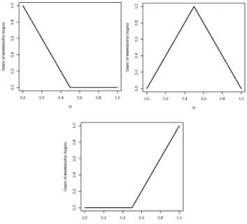
results of aggregating the fuzzy numbers in Figure 2 by a T1OWA operator Φ with the linguistic weights defined in Figure 3 respectively:G¯=ΦAe1,Ae2,Ae3
,Gˆ=ΦBe1,Be2,Be3
. It is clear that for each α ∈[0,1],G¯α−≥Gˆα−, and G¯α+ ≥
ˆ
Gα+, i.e.G¯<Gˆ.
Fig. 3: Linguistic weights of a T1OWA operator:Wf1 (top-left),Wf2 (top-right), and Wf3 (bottom)
Fig. 4: Monotonic relation preserved in the results of aggregating the fuzzy numbers in Fig. 2 by a T1OWA operator defined by the linguistic weights in Fig.3
The next Theorem states that the meet andjoin oper-ators are the lower bound and upper bound of T1OWA aggregation in the sense ofpartial order relation.
Theorem 8. Any T1OWA operator Ψ is between the join, J, and the meet, M:
JAe1,· · ·Aen <ΨAe1,· · ·,Aen <MAe1,· · ·Aen 1 2 3 4 5 6 7 8 9 10 11 12 13 14 15 16 17 18 19 20 21 22 23 24 25 26 27 28 29 30 31 32 33 34 35 36 37 38 39 40 41 42 43 44 45 46 47 48 49 50 51 52 53 54 55 56 57 58 59 60
Proof. According to (3), for each α ∈[0,1], the α-level aggregation of nAei
on
i=1by the T1OWA operator, J, is
Jα e A1α,· · ·,Aenα = n P i=1 wiaσ(i) n P i=1 wi w1∈˜1α, wi∈˜0α (i,1), ai∈Aeiα(∀i)
We have that ˜1α={1}, ˜0α={0}.Thus, Jα e A1α,· · ·,Aenα =naσ(1)|ai∈Aeiα, i= 1,· · ·n o =nmax{a1,· · ·, an}|ai∈Aeiα(∀i) o
As a result, the end points of the α-cut intervals are Jα e A1α,· · ·,Aenα += max e A1α+,· · ·,Aenα+ ; Jα e A1α,· · ·,Aenα −= max e A1α−,· · ·,Aenα−
Theα-level aggregation ofnAei on i=1by a general T1OWA operator Ψ is, ΨαAe1α,· · ·,Aenα = n P i=1 wiaσ(i) n P i=1 wi wi∈Wfαi, ai∈Aeiα(∀i) Furthermore, ΨAe1,· · ·,Aen α+ =ΨαAe1α,· · ·,Aenα + = max f Wαi−≤wi≤Wfαi+ e Aiα−≤ai≤Aeiα+ n P i=1 wiaσ(i) n P i=1 wi = max f Wαi−≤wi≤Wfαi+ n P i=1 wiAe σ(i) α+ n P i=1 wi ≤ max f Wαi−≤wi≤Wfαi+ n P i=1 wimax e A1α+,· · ·,Aenα+ n P i=1 wi = maxAe1α+,· · ·,Aenα+
We have proved that ΨAe1,· · ·,Aen α+ ≤ Jα e A1α,· · ·,Aenα +.Similarly, we have ΨAe1,· · ·,Aen α− ≤ Jα e A1α,· · ·,Aenα −.So we prove that JAe1,· · ·,Aen <ΨAe1,· · ·,Aen
We omit the proof of the other inequality:
Ψ Ae1,· · ·,Aen
< MAe1,· · ·,Aen
, because it follows the same above line of reasoning.
According to Theorem 8, the join and meet operators are two extreme cases of T1OWA operators. T1OWA aggregation is located between themeetand thejoinof all the individual operands, i.e., T1OWA operators are com-pensative: low aggregation in the sense of approaching
the meet operation is compensated by high aggregation in the sense of approaching the joinoperation.
Example 8in theSupplemental Material illustrates the validation of how a T1OWA aggregation maintains the compensative property in terms ofpartial roder relations
of fuzzy numbers.
VI. A Case Study and Experimental Results
A. Diabetes Diagnosis by T1OWA Based Fuzzy Inference System
T1OWA operators have gained many real-world ap-plications in different domains [10], [12], [13]. In this subsection, we further provide a practical application of T1OWA operators to ‘Pima Indian Diabetes’ for in-tegrated patient diagnosis.
The ‘Pima Indian Diabetes’ dataset [18] describes the clinical conditions of 768 females who develop Type-2 diabetes. All patients in this dataset were women (≥21 years old): 500 (65.1%) healthy and 268 (34.9%) with diabetes. It can be seen that this is an imbal-anced dataset. Eight attributes describe the patients: age (years), plasma glucose concentration (plaGlu), number of times pregnant, triceps skin fold thickness (mm), diastolic blood pressure (mmHg), body mass index (BMI) ((weight in kg)/(height in m2)), 2-hour serum insulin (mmol/L), and diabetes pedigree function. The outcome is a class variable (0 or 1):1=diabetic,0=non-diabetetic.
In contrast to other studies using the ‘Pima Indian Diabetes’ dataset, we take into account two further un-derlying issues with the data. One issue is that clearly this is an imbalanced dataset: hence, the widely used assessment metric,classification rate(CR) (also known as
accuracy), is not appropriate and not reliable to assess such a real clinical scenario. For imbalanced datasets, which are very common in clinical studies, the F1
-score and balanced CR (BCR) are a preferred metric, as they makes more sense than others: F1−score= (2·
recall·precision)/(recall+precision);BCR= (sensitivity+ specif icity)/2.
The second issue is that the majority of the existing studies using this dataset did not consider its underlying missing value problem. Indeed, there are no specifically labelled missing values in the dataset. But this cannot be the case, because so many zeros are used to represent the status of attributes where they are biologically impos-sible, such as the attributes of glucose concentration (5 records of zeros), triceps skin fold thickness (227 records of zeros), blood pressure (35 records of zeros), insulin (374 records of zeros), and body mass index (11 records of zeros). It is highly plausible that these zero values were actually originally used to encode missing values in these fields. In our study, we considered these zeros as missing values and used the nearest-neighbor method to impute them. Then we apply different T1OWA aggre-gations to non-stationary fuzzy sets [16], [17] to find the optimal diagnoses of diabetes.
Given a standard fuzzy system as a baseline sys-tem, the T1OWA based non-stationary fuzzy system
1 2 3 4 5 6 7 8 9 10 11 12 13 14 15 16 17 18 19 20 21 22 23 24 25 26 27 28 29 30 31 32 33 34 35 36 37 38 39 40 41 42 43 44 45 46 47 48 49 50 51 52 53 54 55 56 57 58 59 60
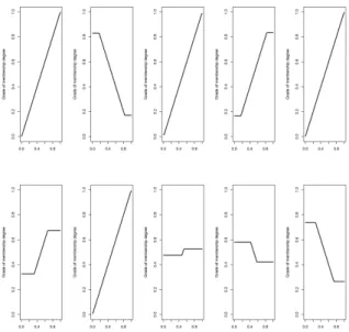
(T1OWANFS) (see Figure 8 in theSupplemental Material) proceeds as follows. First, in each run, the crisp num-bers of each input variable are fuzzified by a fuzzifier function, such as singleton or non-singleton function. These fuzzified input sets then feed into the inference engine with the given rulebase to conduct operations of union and intersection on these fuzzy sets, and perform composition of the relations. Such a process is repeated n runs, so n fuzzy set outputs are produced. Then a T1OWA aggregation operation is applied to these sets to achieve an overall solution. Finally, a crisp output is generated via defuzzification of this overall output fuzzy set.
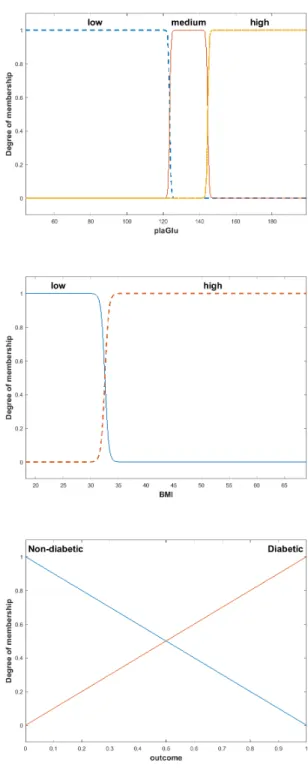
The rulebase in this study consists of the following four rules based on two attributes of plaGluandBMI:
1) Rule 1: if (plaGlu is high) then Diabetic;
2) Rule 2: if (plaGlu is medium) and (BMI is high) then Diabetic;
3) Rule 3: if (plaGlu is low) then Non-Diabetic;
4) Rule 4: if (plaGlu is medium) and (BMI is low) then Non-Diabetic.
where the variables plaGlu, BMI and outcome are de-scribed by baseline fuzzy sets (see Figure 9 of the Sup-plemental Material). Their corresponding non-stationary fuzzy sets were generated based on these baseline sets [16], [17]. In our study, the non-stationary fuzzy sys-tem ran ten times to generate the diagnoses for each patient (Figure 10 in the Supplemental Material shows an example of ten fuzzy decision outputs for a patient). The system performance is evaluted in terms ofF1-score
and BCR.
We use five different types of T1OWA operators in this case study to aggregate the fuzzy diagnosis from non-stationary fuzzy inference engine (see Figure 8 in the
Supplemental Material):
1) the standardjoinoperator: denoted asjoin NFS; 2) the standardmeetoperator: denoted as meet NFS; 3) join-like T1OWA operators with the linguistic
weightWf1 as in Figure 3a and othersWfi(i,1) as in Figure 3b in the Supplemental Materialto aggregate the 10 output sets for diabetes diagnosis: denoted
asJLT1OWA NFS;
4) meet-like T1OWA operators with the last linguistic weightWf10 as in Figure 3a and othersWfi(i,10) as in Figure 3b in the Supplemental Material: denoted
asMLT1OWA NFS;
5) a T1OWA operator with linguistic weights
implementing the fuzzy majority represented by the type-2 quantifier ‘most’ [4]: denoted as
T2MT1OWA NFS.
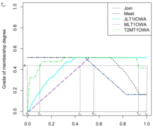
Figure 5 depicts an example of corresponding results of aggregating ten fuzzy decisions from non-stationary fuzzy inference engine for one patient (See Figure 10 in the Supplemental Material) by the above five T1OWA operators. These aggregated fuzzy outputs are then de-fuzzified to generate crisp values as final outputs.
The above examples demonstrate the advantages of these T1OWA operators to aggregate the uncertain infor-mation modelled by fuzzy sets. The T2MT1OWA NFS
operator implements the ‘soft’ majority in aggregating a group of uncertain decisions (perhaps expressed linguis-tically as“most of the decisions should be satisfied”), which is much closer to the real human perception in decision making than traditional aggregation methods. Figure 11 in the Supplemental Material illustrates the joinness
of the operator,T2MT1OWA NFS, which clearly shows that the quantifier ‘most’ guided operator approaches the meet operation (expressed linguistically as“all decisions should be satisfied”). As a matter of fact, such a linguistic quantifier based aggregation can be treated as a mani-festation of a semantically guided aggregation [2], [4].
Fig. 5: Example of aggregation results of 10 fuzzy output decisions (from non-stationary fuzzy inference engine for a patient) by the five different T1OWA operators.
To validate the compensative property of these T1OWA operators, let us assume the aggregation results of the five operators shown in Figure 5 (join NFS,meet NFS,JLT1OWA NFS,MLT1OWA NFS
andT2MT1OWA NFS) be represented aseJ,M,e JL,e ML,g andTe, respectively. TakingT2MT1OWA NFS as an ex-ample, for any α level in Figure 5, it can be seen that
eJα+≥Teα+≥Meα+andeJα−≥Teα−≥Meα−∀α∈[0,1]
Therefore, according to Definition 5, and because the relations < and e≥ are equivalent, we geteJ < Te < M,e i.e., the T2MT1OWA operator verifiesTheorem8, and the
compensative property holds in this case study.
Furthermore, we show a comparison (in terms of F1
-score and BCR) with the following existing methods: (i) standard fuzzy weighted average (FWA) operators [19]; and (ii) a zero-order Takagi-Sugeno fuzzy system with two rules (TSFSTR) [20]. Table I summarises the performances of these approaches. It can be seen that the
1 2 3 4 5 6 7 8 9 10 11 12 13 14 15 16 17 18 19 20 21 22 23 24 25 26 27 28 29 30 31 32 33 34 35 36 37 38 39 40 41 42 43 44 45 46 47 48 49 50 51 52 53 54 55 56 57 58 59 60
TABLE I: Performances of different approaches to diabetes diagnosis
Approach CR Recall Specificity Precision F1-score BCR
Meet NFS 0.760 0.519 0.890 0.716 0.602 0.704 MLT1OWA NFS 0.760 0.519 0.890 0.716 0.602 0.704 T2MT1OWA NFS 0.759 0.586 0.852 0.680 0.629 0.719 JLT1OWA NFS 0.746 0.683 0.780 0.625 0.652 0.731 Join NFS 0.746 0.683 0.780 0.625 0.652 0.731 FWA 0.751 0.619 0.822 0.651 0.635 0.721 TSFSTR 0.716 0.455 0.856 0.629 0.528 0.656
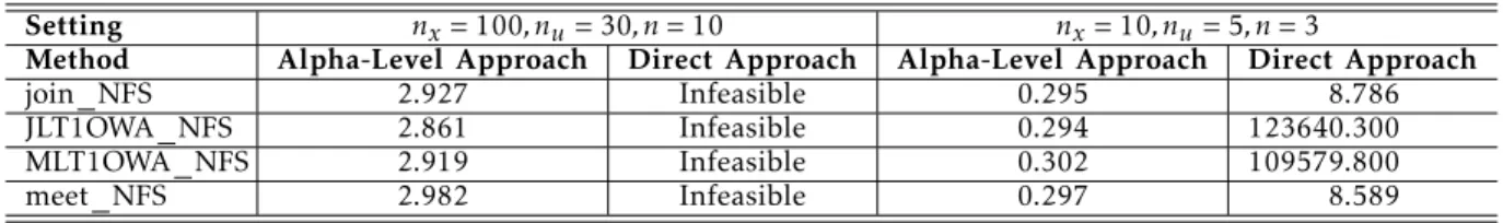
TABLE II: Time-costs of Type-1 OWA Aggregations for Diabetes Diagnoses (in minutes) Setting nx= 100, nu= 30, n= 10 nx= 10, nu= 5, n= 3
Method Alpha-Level Approach Direct Approach Alpha-Level Approach Direct Approach
join NFS 2.927 Infeasible 0.295 8.786
JLT1OWA NFS 2.861 Infeasible 0.294 123640.300
MLT1OWA NFS 2.919 Infeasible 0.302 109579.800
meet NFS 2.982 Infeasible 0.297 8.589
JLT1OWA NFS and joinachieved the best performance in terms of F1-score and BCR. The JLT1OWA NFS
sig-nificantly improved the recall without sacrificing much precision, so that a betterF1-score was achieved. B. Validation of Computing Efficiencies of Alpha-Level Ap-proach to T1OWA Operations in Real World Applications
The Direct Approach [4] and Alpha-Level Approach [5] generate the same results of aggregating fuzzy sets as shown in theRepresentation Theorem of Type-1 OWA Op-erators (Theorem 1). However, theDirect Approachis an exponential-time algorithm that takesO(Kn) operations [5], in which the constant K depends onnu·nx, where n is the number of fuzzy sets to be aggregated, nu is the number of sampling points on the domain [0, 1] of the T1OWA operator’s linguistic weights, and nx is the number of sampling points on the domain of the fuzzy sets to be aggregated. In comparison, the Alpha-Level Approach is a linear-time algorithm, taking O(n) operations [5]. Therefore, the Alpha-Level Approach can be used to implement T1OWA aggregations in real-time applications.
In the subsection VI-A, the T1OWA based fuzzy deci-sion making for diabetes was implemented by the Alpha-Level Approach. The domains of the linguistic weights and fuzzy sets have to be discretized. The default settings are: nu = 30 and nx= 100, while n= 10 (i.e. ten fuzzy decisions). However, such settings are unworkable for the Direct Approach in implementation due to the over-sized vectors which need to be created by the computer. For comparison, therefore, simplified settings are used, such that nu = 5 andnx= 10, while n= 3. Even under such simplified settings, it is estimated that the Direct Approachstill takes days to complete the diagnoses for all 768 patients using themeet-likeorjoin-likeT1OWA oper-ators. Our solution to calculation of time-cost was: firstly, the time-cost,tc1, of the Direct Approachto aggregating
three fuzzy decisions for only one patient is calculated;
then, the total time-cost is 768·tc1. Table II shows the time-costs of the two approaches to diagnosing diabetic patients by the T1OWA operators,join NFS,meet NFS,
JLT1OWA NFS and MLT1OWA NFS. This validated
that the Alpha-Level Approach can achieve much higher computing efficiency than theDirect Approachto aggre-gating fuzzy sets in the manner of OWA operation in real-world applications.
The experimental results were generated in R on a computer with Intel(R) Core [email protected] and 16GB memory. TheRcodes for type-1 OWA aggregations are available upon request.
VII. Discussion and Conclusion
As a generalization of Yager’s OWA operator, T1OWA operators provide an efficient tool to aggregate uncertain information modelled by fuzzy sets in soft decision making. By appropriately selecting fuzzy sets for the weights, various forms of T1OWA operators can be created to fulfill different tasks under multi-granular linguistic contexts. This has been demonstrated in the above case study of diabetic diagnosis, which is an imbalanced data problem. By appropriately selecting the uncertain weights to favour the rare class, such as the join-likeT1OWA operator for the diabetic class, the T1OWA aggregation approach has the potential to en-able standard classifiers to be a cost-sensitive approach, whereby the cost of misclassifying the rare class is higher than the cost of misclassifying the other class. This topic merits further research. In addition, to date, T1OWA operators only consider the norm (minimum) and t-conorm (maximum); but how T1OWA aggregations and properties vary by using different forms of t-norm and t-conorm is an interesting research problem.
In summary, this paper has proven that T1OWA oper-ators verify the same properties which hold for Yager’s OWA operator, namely: idempotence, monotonicity, com-pensativeness, andcommutativity. Such theoretical
analy-1 2 3 4 5 6 7 8 9 10 11 12 13 14 15 16 17 18 19 20 21 22 23 24 25 26 27 28 29 30 31 32 33 34 35 36 37 38 39 40 41 42 43 44 45 46 47 48 49 50 51 52 53 54 55 56 57 58 59 60
ses provide a solid foundation for T1OWA operators to be applied widely in different scenarios.
References
[1] D. H. Hong and S. Han, “The General Least Square Devi-ation OWA Operator Problem,” Mathematics 2019, 7(4), 326; doi:10.3390/math7040326 .
[2] R. R. Yager, “On ordered weighted averaging aggregation oper-ators in multi-criteria decision making,”IEEE Trans. on Systems, Man and Cybernetics, vol.18, pp.183-190, 1988.
[3] A. Kishor, A. K. Singh, A. Sonam, N. Pal, “A New Family of OWA Operators Featuring Constant Orness,” IEEE Trans. on Fuzzy Systems, 2020 (Appearing).
[4] S.-M. Zhou, F. Chiclana, R. I. John, and J. M. Garibaldi, “Type-1 OWA operators for aggregating uncertain information with uncertain weights induced by type-2 linguistic quantifiers,” Fuzzy Sets and Systems, vol.159, no.24, pp.3281-3296, 2008. [5] S.-M. Zhou, F. Chiclana, R. I. John, and J. M. Garibaldi,
“Alpha-Level Aggregation: A Practical Approach to Type-1 OWA Oper-ation for Aggregating Uncertain InformOper-ation with ApplicOper-ations to Breast Cancer Treatments,” IEEE Trans. on Knowledge and Data Engineering, vol.23, issue 10, pp. 1455 - 1468, 2011. [6] L. A. Zadeh, “The concept of a linguistic variable and its
application to approximate reasoning-2,” Information Science, vol. 8, pp. 301-357, 1975.
[7] J. M. Mendel and R. I. John, “Type-2 fuzzy sets made simple,” IEEE Trans. on Fuzzy Systems, vol.10, no.2, pp.117-127, 2002. [8] S.-M. Zhou, J. M. Garibaldi, R. I. John and F. Chiclana, “On
constructing parsimonious type-2 fuzzy logic systems via in-fluential rule selection,” IEEE Trans. on Fuzzy Systems, vol.17, no.3, pp.654-667, 2009.
[9] D. Wu, J. Huang, “Ordered Novel Weighted Averages,” In: John et al (eds)Type-2 Fuzzy Logic and Systems. Studies in Fuzziness and Soft Computing, vol 362. Springer, 2018.
[10] A.R. Buck, J.M. Keller, M. Popescu, “Anα-Level OWA Imple-mentation of Bounded Rationality for Fuzzy Route Selection,” In: Jamshidi M., Kreinovich V., Kacprzyk J. (eds)Advance Trends in Soft Computing. Studies in Fuzziness and Soft Computing, vol 312. Springer, 2014.
[11] H. Hu, Q. Yang, Y. Cai, “An opposite direction searching al-gorithm for calculating the type-1 ordered weighted average,” Knowledge-Based Systems52 (2013) 176-180
[12] F. Chiclana, F. Mata, L. G. Perez, E. Herrera-Viedma, ”Type-1 OWA Unbalanced Fuzzy Linguistic Aggregation Methodology: Application to Eurobonds Credit Risk Evaluation,”International Journal of Intelligent Systems, Vol. 33, 1071-1088, 2018. [13] F. Mata, L. G. Perez, S.-M. Zhou, and F. Chiclana, “Type-1
OWA methodology to consensus reaching processes in multi-granular linguistic contexts,”Knowledge-Based Systems, Volume 58, March 2014, Pages 11-22
[14] F. Chiclana, S.-M. Zhou, “Type-reduction of general type-2 fuzzy sets: The type-1 OWA method,” International Journal of Intelligent Systems, vol. 28, pp.505 - 522, 2013
[15] J. Ramik and J. Rimanek, “Inequality relation between fuzzy numbers and its use in fuzzy operation,”Fuzzy Sets and Systems, vol.16, pp. 123-138, 1985.
[16] J. M. Garibaldi and T. Ozen, “Uncertain fuzzy reasoning: a case study in modelling expert decision making,”IEEE Trans. Fuzzy Systems, vol.15, pp.16-30, 2007.
[17] J. M. Garibaldi, M. Jaroszewski and S. Musikasuwan, “Non-stationary fuzzy sets,” IEEE Trans. Fuzzy Systems, vol.16, pp.1072-1086, 2008.
[18] UCI repository of machine learning databases, J. Mertz and P. M. Murphy. [Online]. Available: http://www.ics.uci.edu/pub/machinelearning-data-bases [19] F. Liu and J. M. Mendel. “Aggregation Using the Fuzzy Weighted
Average as Computed by the Karnik–Mendel Algorithms,”IEEE Trans. on Fuzzy Systems, vol.16, issue 1, Feb. 2008, pp. 1 - 12 [20] N. Settouti, M. A. Chikh, and M. Saidi,“Generating fuzzy rules
for constructing interpretable classifier of diabetes disease,” Australasian physical and engineering sciences in medicine 35(3):257-70,August 2012 1 2 3 4 5 6 7 8 9 10 11 12 13 14 15 16 17 18 19 20 21 22 23 24 25 26 27 28 29 30 31 32 33 34 35 36 37 38 39 40 41 42 43 44 45 46 47 48 49 50 51 52 53 54 55 56 57 58 59 60
Supplemental Material for the Manuscript
“Type-1 OWA Operators in Aggregating Multiple
Sources of Uncertain Information : Properties
and Real World Applications”
Shang-Ming Zhou,
Member, IEEE,
Francisco Chiclana, Robert I. John,
Senior Member, IEEE,
Jon M. Garibaldi,
Senior Member, IEEE,
and Lin Huo
I. MORE EXAMPLES OFTYPE-1 OWA AGGREGATIONS
Example 1(A T1OWA Operator). Figure 1 depicts the results of a T1OWA operator to aggregate four fuzzy sets. Figure 1a shows the linguistic weights. Figure 1b shows the aggregated fuzzy set objects and aggregation result.
(a) Fuzzy sets as linguistic weights in T1OWA aggre-gation 0 1 2 3 4 0.0 0.2 0.4 0.6 0.8 1.0 X
Grade of membership degree
(b) Aggregation result in dashed lines; aggregated fuzzy set objects in solid lines
Fig. 1: A T1OWA operator
Example 2 (Join Operator). Figure 2 illustrates the result of join operator to aggregate fuzzy sets as the extended maximum of fuzzy sets, a special T1OWA operator.
0 1 2 3 4 0.0 0.2 0.4 0.6 0.8 1.0 X
Grade of membership degree
(a) Fuzzy sets to be aggregated
0 1 2 3 4 0.0 0.2 0.4 0.6 0.8 1.0 X
Grade of membership degree
(b) Aggregating result
Fig. 2: Aggregation of T1OWA operator as join
Example 3 (Join-Like T1OWA Operator). The Join-like T1OWA operation requests that the first linguistic weight move towards the singleton fuzzy set,˜1, and all others towards the singleton fuzzy set˜0 (Figure 4a and Figure 4b). Using these weights to aggregate the fuzzy sets, Figure 3c illustrates how this T1OWA exhibits the join-like behaviour when aggregating three fuzzy sets. Clearly, the final aggregation fuzzy set is closer to the rightmost fuzzy set (i.e., the fuzzified maximum)
1 2 3 4 5 6 7 8 9 10 11 12 13 14 15 16 17 18 19 20 21 22 23 24 25 26 27 28 29 30 31 32 33 34 35 36 37 38 39 40 41 42 43 44 45 46 47 48 49 50 51 52 53 54 55 56 57 58 59 60
(a)fW1 (b)Wfi(i6= 1)
(c) Aggregation result
Fig. 3: A join-like T1OWA operator. (a)(b)-Linguistic weights;(c)-Aggregation result. Solid lines representing the aggregated objects; dashed line representing the aggregation result.
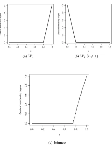
Example 4 (Joinness of Join-Like T1OWA Operator). The Figure 4c shows an example of the joinness of the join-like T1OWA operator defined by the fuzzy weights in Figure 4a and Figure 4b.
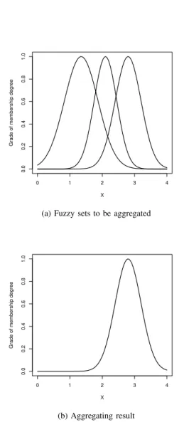
Example 5(Meet Operator). Figure 5 illustrates the result of meet operator to aggregate fuzzy sets as the extended minimum of fuzzy sets, a special T1OWA operator.
Example 6(Meet-Like T1OWA Operator). Meet-like T1OWA operation requests that the last linguistic weight to be close to ˜1 (Figure 4a), and all other weights close to ˜0 (Figure 4b). Figure 6 illustrates how this T1OWA exhibits the meet-like behaviour when aggregating three fuzzy sets. Clearly, the final aggregation fuzzy set is closer to the leftmost fuzzy set (i.e., the fuzzified minimum).
Example 7 (Counterexample of α-Equivalently Ordered
Relation). Figure 7 shows the groups of fuzzy numbers
{Be1,Be2,Be3} are not α-equivalently ordered with another
group {Ae1,Ae2,Ae3}. Figure 7a shows that at the α = 0.2
level:Ae30.2+≥Ae20.2+≥Ae10.2+, i.e., the permutation operator
σ = (3,2,1), but Be0.2+3 ≥ Be0.2+1 ≥ Be0.2+2 ; while Fig.7b
shows that Ae30.2− ≥ Ae20.2− ≥ Ae10.2−, i.e., the permutation
operator η= (3,2,1), butBe0.23 −≥Be0.21 −≥Be0.22 −.
Example 8. Supposing the numerical domains U =
(a)W1 (b)Wi(i6= 1) 0.0 0.2 0.4 0.6 0.8 1.0 0.0 0.2 0.4 0.6 0.8 1.0 v
Grade of membership degree
(c) Joinness
Fig. 4:Joinnessof a join-like T1OWA operator
{0.0,0.5,1.0} andX ={0.0,1.0,2.0}. Let the given linguis-tic weightsWf= ωi µ f W(ωi) ωi∈U onU be f W1= 0.0 0.5 1.0 1.0 0.5 0.0 ; Wf2= 0.0 0.5 1.0 0.0 1.0 0.0 ; f W3= 0.0 0.5 1.0 0.0 0.5 1.0
and the fuzzy sets to be aggregated be
e A1= 0.0 1.0 2.0 0.0 0.5 1.0 ; Ae2= 0.0 1.0 2.0 1.0 0.5 0.0 ; e A3= 0.0 1.0 2.0 0.0 1.0 0.0
The aggregation result by the join operator J can be calcu-lated as follows. 1) Forα= 0.0, JαAe1α,Ae2α,Ae3α += max e A1α+,Ae2α+,Ae3α+ = 2.0 Jα e A1 α,Ae2α,Ae3α −= max e A1 α−,Ae2α−,Ae3α− = 0.0 So Gα−≤Jα−, Gα+≤Jα+. 1 2 3 4 5 6 7 8 9 10 11 12 13 14 15 16 17 18 19 20 21 22 23 24 25 26 27 28 29 30 31 32 33 34 35 36 37 38 39 40 41 42 43 44 45 46 47 48 49 50 51 52 53 54 55 56 57 58 59 60
0 1 2 3 4 0.0 0.2 0.4 0.6 0.8 1.0 X
Grade of membership degree
(a) Fuzzy sets to be aggregated
0 1 2 3 4 0.0 0.2 0.4 0.6 0.8 1.0 X
Grade of membership degree
(b) Aggregating result
Fig. 5: Aggregation of T1OWA operator as meet
Fig. 6: Aggregation result by a meet-like T1OWA operator. Solid lines representing the aggregated objects; dashed line representing the aggregation result.
(a)Ae30.2+ ≥Ae20.2+ ≥ Ae01.2+ and Be03.2+ ≥Be01.2+ ≥ e B2 0.2+ (b)Ae30.2− ≥Ae20.2− ≥Ae01.2−and Be03.2−≥Be01.2− ≥ e B2 0.2−
Fig. 7: Fuzzy numbersBe1,Be2,Be3(bottom) notα-equivalently
ordered withAe1,Ae2,Ae3 (up) separately
2) Forα= 0.5, Jα e A1 α,Ae2α,Ae3α + = maxAe1α+,Ae2α+,Ae3α+ = max{2.0,1.0,1.0} = 2.0 JαAe1α,Ae2α,Ae3α −= max e A1 α−,Ae2α−,Ae3α− = max{1.0,0.0,1.0} = 1.0 SoGα−≤Jα−, Gα+≤Jα+. 3) Forα= 1.0 JαAe1α,Ae2α,Ae3α += max e A1α+,Ae2α+,Ae3α+ = max{2.0,0.0,1.0} = 2.0 Jα e A1 α,Ae2α,Ae3α −= max e A1 α−,Ae2α−,Ae3α− = max{2.0,0.0,1.0} = 2.0 So Gα−≤Jα−, Gα+≤Jα+.
Then according to the Definition about partial order relation of fuzzy sets, we have J < G. Similarly,G < M, the meet operator. 1 2 3 4 5 6 7 8 9 10 11 12 13 14 15 16 17 18 19 20 21 22 23 24 25 26 27 28 29 30 31 32 33 34 35 36 37 38 39 40 41 42 43 44 45 46 47 48 49 50 51 52 53 54 55 56 57 58 59 60
II. CASESTUDY
A. The T1OWA based non-stationary fuzzy system
Figure 8 illustrates the structure of T1OWA based non-stationary fuzzy inference system, the T1OWA operator is used to aggregate the multiple fuzzy decisions from non-stationary fuzzy inference engine.
Fig. 8: T1OWA based non-stationary fuzzy inference system
B. Fuzzy sets of the variables - ”plaGlu”, ”BMI” and ”Out-come”
joinnessOfT2QuantMostPrecision0d0035
Fig. 9: Membership functions of fuzzy sets for the attributes of plaGlu, BMI and outcome
1 2 3 4 5 6 7 8 9 10 11 12 13 14 15 16 17 18 19 20 21 22 23 24 25 26 27 28 29 30 31 32 33 34 35 36 37 38 39 40 41 42 43 44 45 46 47 48 49 50 51 52 53 54 55 56 57 58 59 60
(a) 10 fuzzy output decisions
Fig. 10: Example of 10 fuzzy output decisions by the non-stationary fuzzy system for a patient
Fig. 11: Joinness of the type-2 quantifier ”most” guided T1OWA operator 1 2 3 4 5 6 7 8 9 10 11 12 13 14 15 16 17 18 19 20 21 22 23 24 25 26 27 28 29 30 31 32 33 34 35 36 37 38 39 40 41 42 43 44 45 46 47 48 49 50 51 52 53 54 55 56 57 58 59 60