Efficient Large Scale Clustering based on Data
Partitioning
Malika Bendechache
Insight Centre for Data AnalyticsSchool of Computer Science University College Dublin
Dublin, Ireland
Email: [email protected]
Nhien-An Le-Khac
School of Computer ScienceUniversity College Dublin Dublin, Ireland Email: [email protected]
M-Tahar Kechadi
Insight Centre for Data AnalyticsSchool of Computer Science University College Dublin
Dublin, Ireland Email: [email protected]
Abstract—Clustering techniques are very attractive for ex-tracting and identifying patterns in datasets. However, their appli-cation to very large spatial datasets presents numerous challenges such as high-dimensionality data, heterogeneity, and high com-plexity of some algorithms. For instance, some algorithms may have linear complexity but they require the domain knowledge in order to determine their input parameters. Distributed clustering techniques constitute a very good alternative to the big data challenges (e.g.,Volume, Variety, Veracity, and Velocity). Usually these techniques consist of two phases. The first phase generates local models or patterns and the second one tends to aggregate the local results to obtain global models. While the first phase can be executed in parallel on each site and, therefore, efficient, the aggregation phase is complex, time consuming and may produce incorrect and ambiguous global clusters and therefore incorrect models. In this paper we propose a new distributed clustering approach to deal efficiently with both phases; generation of local results and generation of global models by aggregation. For the first phase, our approach is capable of analysing the datasets located in each site using different clustering techniques. The aggregation phase is designed in such a way that the final clusters are compact and accurate while the overall process is efficient in time and memory allocation. For the evaluation, we use two well-known clustering algorithms; K-Means and DBSCAN. One of the key outputs of this distributed clustering technique is that the number of global clusters is dynamic; no need to be fixed in advance. Experimental results show that the approach is scalable and produces high quality results.
Keywords—Big Data, spatial data, clustering, distributed min-ing, data analysis, k-means, DBSCAN.
I. INTRODUCTION
Currently, one of the most critical data challenges which has a massive economic need is how to efficiently mine and manage all the data we have collected. This is even more critical when the collected data is located on different sites, and are owned by different organisations [1]. This led to the development of distributed data mining (DDM) techniques to deal with huge, multi-dimensional and heterogeneous datasets, which are distributed over a large number of nodes. Existing DDM techniques are based on performing partial analysis on local data at individual sites followed by the generation of global models by aggregating these local results. These two steps are not independent since naive approaches to local analysis may produce incorrect and ambiguous global data models. In order to take advantage of the mined knowledge at
different locations, DDM should have a view of the knowledge that not only facilitates their integration, but also minimises the effect of the local results on the global models. Briefly, an efficient management of distributed knowledge is one of the key factors affecting the outputs of these techniques [2], [3], [4], [5]. Moreover, the data that is collected and stored in different locations using different instruments may have different formats and features. Traditional, centralised data mining techniques have not considered all the issues of data-driven applications, such as scalability in both response time and accuracy of solutions, distribution, and heterogeneity [6]. Some DDM approaches are based on ensemble learning, which uses various techniques to aggregate the results [7], among the most cited in the literature: majority voting, weighted voting, and stacking [8], [9].
DDM is more appropriate for large scale distributed plat-forms, where datasets are often geographically distributed and owned by different organisations. Many DDM methods such as distributed association rules and distributed classification [10], [11], [12], [3], [13], [14] have been proposed and developed in the last few years. However, only a few researches concern distributed clustering for analysing large, heterogeneous and distributed datasets. Recent researches [15], [16], [17] have proposed distributed clustering approaches based on the same 2-step process: perform partial analysis on local data at indi-vidual sites and then aggregate them to obtain global results. In this paper, we propose a distributed clustering approach based on the same 2-step process, however, it reduces significantly the amount of information exchanged during the aggregation phase, and generates automatically the correct number of clusters. A case study of an efficient aggregation phase has been developed on spatial datasets and proven to be very efficient; the data exchanged is reduced by more than 98%
of the original datasets [18].
The approach can use any clustering algorithm to per-form the analysis on local datasets. As can be seen in the following sections, we tested the approach with two well-known centroid-based and density-based clustering algorithms (K-Means and DBSCAN, respectively), and the results are of very high quality. More importantly, this study shows how importance of the local mining algorithms, as the local clusters accuracy affects heavily the quality of the final models.
next section we will give an overview of the state-of-the-art for distributed data mining and discuss the limitations of traditional techniques. Then we will present the proposed dis-tributed framework and its concepts in Section III. In Section IV, we evaluated the distributed approach using two well-known algorithms; K-Means and DBSCAN. We discuss more experimental results showing the quality of our algorithm’s results in Section V. Finally, we conclude in Section VI.
II. RELATEDWORK
Distributed Data Mining (DDM) is a line of research that has attracted much interest in recent years [19]. DDM was developed because of the need to process data that can be very large or geographically distributed across multiple sites. This has two advantages: first, a distributed system has enough power to analyse the data within a reasonable time frame. Second, it would be very advantageous to process data on their respective sites to avoid the transfer of large volumes of data to a central site to avoid heavy communications, network bottlenecks, etc.
DDM techniques can be divided into two categories based on the targeted architectures of computing platforms [20]. The first, based on parallelism, uses traditional dedicated and parallel machines with tools for communications between pro-cessors. These machines are generally called super-computers and are very expensive. The second category targets a network of autonomous machines. These are called distributed systems, and are characterised by a distributed communication network connecting low-speed machines that can be of different archi-tectures, but they are very abundant [21]. The main goal of the second category of techniques is to distribute the work among the system nodes and try to minimise the response time of the whole application. Some of these techniques have already been developed and implemented in [22], [23].
However, the traditional DDM methods are not always effective, as they suffer from the problem of scaling. This has led to the development of techniques that rely on ensemble learning [24], [25]. These new techniques are very promising. Integrating ensemble learning methods in DDM, will allow to deal with the scalability problem. One solution to deal with large scale data is to use parallelism, but this is very expensive in terms of communications and processing power. Another solution is to reduce the size of training sets (sampling). Each system node generates a separate sample. These samples will be analysed using a single global algorithm [26], [27]. However, this technique has a disadvantage that the sampling depends on the transfer time which may impact on the quality of the samples.
Clustering algorithms can be divided into two main cate-gories, namely partitioning and hierarchical. Different elabo-rated taxonomies of existing clustering algorithms are given in the literature. Many parallel clustering versions based on these algorithms have been proposed in the literature [17], [28], [29], [30], [31], [32], [33]. These algorithms are further classified into two sub-categories. The first consists of methods requiring multiple rounds of message passing. They require a significant amount of synchronisations. The second sub-category consists of methods that build local clustering models and send them to a central site to build global models [18]. In
[28] and [32], message-passing versions of the widely used K-Means algorithm were proposed. In [29] and [33], the authors dealt with the parallelisation of the DBSCAN density-based clustering algorithm. In [30] a parallel message passing version of the BIRCH algorithm was presented. A parallel version of a hierarchical clustering algorithm, called MPC for Message Passing Clustering, which is especially dedicated to Microarray data was introduced in [31]. Most of the parallel approaches need either multiple synchronisation constraints between processes or a global view of the dataset, or both [17].
Another approach presented in [17] also applied a merg-ing of local models to create the global models. Current approaches only focus on either merging local models or mining a set of local models to build global ones. If the local models cannot effectively represent local datasets then global models accuracy will be very poor [18]. Both partitioning and hierarchical categories suffer from some drawbacks. For the partitioning class, K-Means algorithm needs the number of clusters fixed in advance, while in the majority of cases K
is not known. Furthermore, hierarchical clustering algorithms have overcome this limit: they do not need to provide the number of clusters as an input parameter, but they must define the stopping conditions for clustering decomposition, which is not an easy task.
III. DYNAMICDISTRIBUTEDCLUSTERING
We first describe the proposed Dynamic Distributed Clus-tering (DDC) model, where the local models are based on the boundaries of clusters. We also present an evaluation of the approach with different local clustering techniques including centroid-based (K-Means) and density-based (DBSCAN) tech-niques.
The DDC approach includes two main steps. In the first step, as usual, we cluster the datasets located on each node of the system and select good local representatives. This phase is executed in parallel without communications between the nodes. In this phase we can reach a super speed-up. The next phase, however, collects the local models from each node and affects them to some special nodes in the system called leaders. The leaders are elected according to some characteristics such as their capacity, processing power, connectivity, etc. The leaders are responsible for merging and regenerating the data objects based on the local cluster representatives. The purpose of this step is to improve the quality of the global clusters, as usually the local clusters do not contain enough important information.
A. Local Models
The local clusters are highly dependent on the clustering techniques used by their corresponding nodes. For instance, for spatial datasets, the shape of a cluster is usually dictated by the technique used to obtain them. Moreover, this is not an issue for the first phase, as the accuracy of a cluster affects only the local results of a given node. However, the second phase requires sending and receiving all local clusters to the leaders. As the whole data is very large, this operation will saturate very quickly the network. So, we must avoid sending all the original data through the network. The key idea behind the DDC approach is to send only the cluster’s representatives, which constitute between 1%and2% of the total size of the data. The cluster representatives consist of the internal data representatives plus the boundary points of the cluster.
There are many existing data reduction techniques in the literature. Many of them are focusing only on the dataset size i.e., they try to reduce the storage capacity without paying attention to the knowledge contained in the data. In [34], an efficient reduction technique has been proposed; it is based on density-based clustering algorithms. Each cluster is represented by a set of carefully selected data-points, called representatives. However, selecting representatives is still a challenge in terms of quality and size [15], [18].
The best way to represent a spatial cluster is by its shape and density. The shape of a cluster is represented by its boundary points (called contour) (see Figure 1). Many algorithms for extracting the boundaries from a cluster can be found in the literature [35], [36], [37], [38], [39]. We used the algorithm proposed in [40], which is based on triangulation to generate the cluster boundaries. It is an efficient algorithm for constructing non-convex boundaries. The algorithm is able to accurately characterise the shape of a wide range of different point distributions and densities with a reasonable complexity of O(nlogn).
B. Global Models
The global models (patterns) are generated during the second phase of the DDC. This phase is also executed in a distributed fashion but, unlike the first phase, it has commu-nications overheads. This phase consists of two main steps, which can be repeated until all the global clusters were generated. First, each leader collects the local clusters of its neighbours. Second, the leaders will merge the local clusters
using the overlay technique. The process of merging clusters will continue until we reach the root node. The root node will contain the global clusters (see Figure 1).
Note that, this phase can be executed by a clustering algorithm, which can be the same as in the first phase or com-pletely different one. This approach belongs to the category of hierarchical clustering.
As mentioned above, during the second phase, communi-cating the local clusters to the leaders may generate a huge overhead. Therefore, the objective is to minimise the data communication and computational time, while getting accurate global results. In DDC we only exchange the boundaries of the clusters, instead of exchanging the whole clusters between the system nodes.
In the following, we summarise the steps of the DDC ap-proach for spatial data. The nodes of the distributed computing system are organised following a tree topology.
1) Each node is allocated a dataset representing a portion of the scene or of the overall dataset.
2) Each leaf node executes a local clustering algorithm with its own input parameters.
3) Each node shares its clusters with its neighbours in order to form larger clusters using the overlay technique.
4) The leader nodes contain the results of their groups. 5) Repeat 3 and 4 until all global clusters were
gener-ated.
Note that the DDC approach suits very well the MapRe-duce framework, which is widely used in cloud computing systems.
IV. DDC EVALUATION ANDVALIDATION
In order to evaluate the performance of the DDC approach, we use different local clustering algorithms. In this paper we use a centroid-based algorithm (K-Means) and a density-based Algorithm (DBSCAN).
A. DDC-K-Means
Following the general structure of the approach described above, the DDC with K-Means (DDC-K-Means) is charac-terised by the fact that in the first phase, called the parallel phase, each node Ni of the system executes the K-Means
algorithm on its local dataset to produce Li local clusters and calculate their contours. The rest of the process is the same as described above. In other words, the second phase consists of exchanging the contours located in each node with its neighbourhood nodes. Each leader attempts to merge overlapping contours of its group. Therefore, each leader generates new contours (new clusters). The merge procedure will continue until there is no overlapping contours.
It has been shown in [41] that DDC-K-Means dynamically determines the number of the clusters without a priori knowl-edge about the data or an estimation process of the number of the clusters. DDC-K-Means was also compared to two well-known clustering algorithms: BIRCH and CURE. The results showed that the quality of the DDC-K-Means’ clusters is much better that the ones generated by both BIRCH and CURE. As
expected, this approach runs much faster than the two other algorithms; BIRCH and CURE.
To summarise, DDC-K-Means does not need the number of global clusters to be given as an input. It is calculated dynamically. Moreover, each local clusteringLiwith K-Means needs Ki as a parameter, which is not necessarily the exact K for that local clustering. Let K˜i be the exact number of
local clusters in the node Ni, all it is required is to set Ki
such that Ki > Ki˜. This is much simpler than giving Ki, especially when we do not have enough knowledge about the local dataset characteristics. Nevertheless, it is indeed better to set Ki as close as possible to Ki˜ in order to reduce the processing time in calculating the contours and also merging procedure.
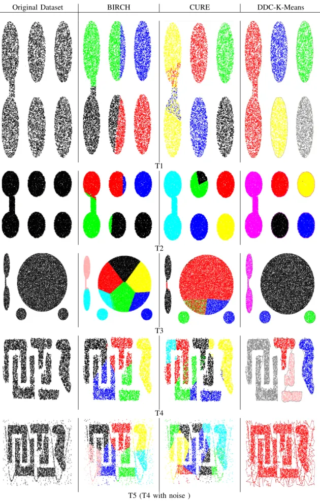
Figure 2 shows a comparative study between DDC-K-Means and two well-known algorithms; BIRCH and CURE. The experiments use five datasets (T1, T2, T3, T4, T5) described in Table I. Note thatT5is the same dataset asT4for which we removed the noise. Each color represents a separate cluster.
As we can see, DDC-K-Means successfully generates the final clusters for the first three datasets (T1, T2 and T3), whereas BIRCH and CURE fail to generate the expected clusters for all the datasets (T1, T2, T3, T4 andT5). However, DDC-K-Means fails to find good clusters for the two last datasets (T4 andT5), this is due to the fact that the K-Means algorithm tends to work with convex shape only, because it is based on the centroid principle to generate clusters. Moreover, we can also notice that the results of DDC-K-Means are even worse with dataset which contains noise (T5). In fact it returns
the whole dataset with the noise as one final cluster for each dataset (see Figure 2). This is because K-Means does not deal with noise.
B. DDC with DBSCAN
While, the DDC-K-Means performs much better than some well-known clustering algorithms on spatial datasets, it still can not deal with all kinds of datasets; mainly with non-convex shapes. In addition, DDC-K-Means is very sensitive to noise. Therefore, instead of K-Means, we use another clustering algorithm for spatial datasets, which is DBSCAN. DBSCAN is summarised below.
1)DBSCAN: DBSCAN (Density-Based spatial Cluster-ing of Applications with Noise) is a well-known density based clustering algorithm capable of discovering clusters with arbitrary shapes and eliminating noisy data [42]. Briefly, DBSCAN clustering algorithm has two main parameters: the radius Eps and minimum points M inP ts. For a given point
p, the Eps neighbourhood of p is the set of all the points around pwithin distanceEps. If the number of points in the
Eps neighbourhoodofpis smaller thanM inP ts, then all the points in this set, together withp, belong to the same cluster. More details can be found in [42].
Compared with other popular clustering methods such as K-Means [43], BIRCH [44], and STING [45], DBSCAN has several key features. First, it groups data into clusters with arbitrary shapes. Second, it does not require the number of the clusters to be given as an input. The number of clusters is determined by the nature of the data and the values ofEpsand
M inP ts. Third, it is insensitive to the input order of points in the dataset. All these features are very important to any clustering algorithm.
2)DBSCAN Complexity: DBSCAN visits each point of the dataset, possibly multiple times (e.g., as candidates to different clusters). For practical considerations, however, the time complexity is mostly governed by the number of re-gionQuery invocations. DBSCAN executes exactly one such query for each point, and if an indexing structure is used that executes a neighbourhood query in O(logn), an overall average complexity ofO(nlogn)is obtained if the parameter
Epsis chosen in a meaningful way, (i.e., such that on average only O(logn) points are returned). Without the use of an accelerating index structure, or on degenerated data (e.g., all points within a distance less than Eps), the worst case run time complexity remains O(n2). The distance matrix of size O((n2 − n/2)) can be materialised to avoid distance
re-computations, but this needsO(n2)of memory, whereas a
non-matrix based implementation of DBSCAN only needsO(n)of memory space.
3)DDC-DBSCAN Algorithm: The approach remains the same (as explained in Section III), the only difference is at local level (See Figure 1). Where, instead of using K-Means for processing local clusters, we use DBSCAN. Each node (ni) executes DBSCAN on its local dataset to produce
Ki local clusters. Once all the local clusters are determined, we calculate their contours. These contours will be used as representatives of their corresponding clusters.
The second phase consists of exchanging the contours located in each node with its neighbourhood nodes. This will allow us to identify overlapping contours (clusters). Each leader attempts to merge overlapping contours of its group. Therefore, each leader generates new contours (new clusters). We repeat the second and third steps till we reach the root node. The sub-clusters aggregation is done following a tree structure and the global results are located in the top level of the tree (root node). The algorithm pseudo code is given in Algorithm 1.
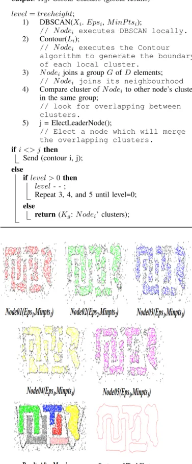
Figure 3 illustrates an example of DDC-DBSCAN. Assume that the distributed computing platform contains five Nodes (N = 5). Each Node executes DBSCAN algorithm with its local parameters (Epsi,M inP tsi) on its local dataset. As it can be seen in Figure 3 the new approach returned exactly the right number of clusters and their shapes. The approach is insensitive to the way the original data was distributed among the nodes. It is also insensitive to noise and outliers. As we can see, although each node executed DBSCAN locally with different parameters. The global final clusters were correct even on the noisy dataset (T5) (See Figure 3).
Original Dataset BIRCH CURE DDC-K-Means T1 T2 T3 T4 T5 (T4 with noise )
Algorithm 1: DDC with DBSCAN.
input : Xi: Dataset Fragment,Epsi: Distance Epsi for
N odei,M inP tsi: minimum points contain clusters generated byN odei,D: tree degree,
Li: Local clusters generated byN odei
output: Kg: Global Clusters (global results)
level=treeheight;
1) DBSCAN(Xi.Epsi,M inP tsi);
// N odei executes DBSCAN locally.
2) Contour(Li);
// N odei executes the Contour algorithm to generate the boundary of each local cluster.
3) N odei joins a group GofD elements;
// N odei joins its neighbourhood
4) Compare cluster ofN odei to other node’s clusters in the same group;
// look for overlapping between clusters.
5) j = ElectLeaderNode();
// Elect a node which will merge the overlapping clusters.
ifi <> j then
Send (contour i, j);
else
iflevel >0then
level- - ;
Repeat 3, 4, and 5 until level=0;
else
return(Kg:N odei’ clusters);
V. EXPERIMENTALRESULTS
In this section, we study the performance of the DDC-DBSCAN approach and demonstrate its effectiveness com-pared to BIRCH, CURE and DDC-K-Means. We choose these algorithms because either they are in the same category as the proposed technique, such as BIRCH which belongs to hier-archical clustering category, or have an efficient optimisation approach, such as CURE.
BIRCH: We used the BIRCH implementation provided in [44]. It performs a pre- clustering and then uses a centroid-based hierarchical clustering algorithm. Note that the time and space complexity of this approach is quadratic to the number of points after pre-clustering. We set its parameters to the default values suggested in [44].
CURE: We used the implementation of CURE provided in [46]. The algorithm uses representative points with shrinking towards the mean. As described in [46], when two clusters are merged in each step of the algorithm, representative points for the new merged cluster are selected from the ones of the two original clusters rather than all the points in the merged clusters.
A. Experiments
We run experiments with different datasets. We used six types of datasets with different shapes and sizes. The first three datasets (T1, T2, andT3) are the same datasets used to evaluate DDC-K-Means. The last three datasets (T4, T5, and
T6) are very well-known benchmarks to evaluate density-based clustering algorithms. All the six datasets are summarised in Table I. The number of points and clusters in each dataset is also given. These six datasets contain a set of shapes or patterns which are not easy to extract with traditional techniques.
TABLE I: The datasets used to test the algorithms. Type Dataset Description #Points #Clusters
Convex
T1 Big oval
(egg shape) 14,000 5
T2 4 small circles
and 2 small circles linked 17,080 5 T3
2 small circles, 1 big circle and 2 linked ovals
30,350 4 Non-Convex with Noise T4 Different shapes including noise 8,000 6 T5
Different shapes, with some clusters surrounded
by others
10,000 9
T6 Letters with noise 8,000 6
B. Quality of Clustering
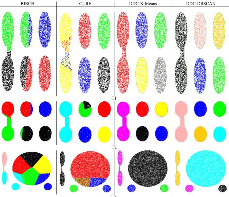
We run the four algorithms on the six datasets in order to evaluate the quality of their final clusters. In the case of the DDC approach we took a system that contains five nodes, therefore, the results shown are the aggregation of the five local clustering. Figure 4 shows the returned clusters by each of the four algorithms for convex shapes of the clusters (T1, T2,
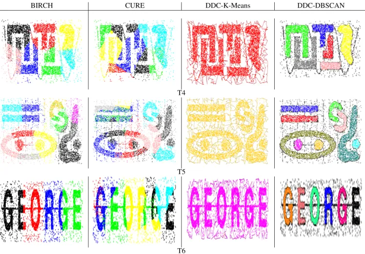
and T3) and Figure 5 shows the clusters returned for
non-convex shapes of the clusters with noise (T4, T5,andT6). We use different colours to show the clusters returned by each algorithm.
BIRCH CURE DDC-K-Means DDC-DBSCAN
T1
T2
T3
Fig. 4: Clusters generated for datasets (T1, T2, T3).
From the results shown in Figure 4, as expected, since BIRCH cannot find all the clusters correctly. It splits the larger cluster while merging the others. In contrast, CURE generates correctly the majority of the final clusters but it still fails to discover all the clusters. Whereas both DDC-K-Means and DDC-DBSCAN algorithms successfully generate all the clusters with the default parameter settings.
Figure 5 shows the clusters generated for the datasets (T4, T5, and T6). As expected, again BIRCH could not find correct clusters; it tends to work better with convex shapes of the clusters. In addition, BIRCH does not deal with noise. The results of CURE are worse and it is not able to extract clusters with non-convex shapes. We can also see that CURE does not deal with noise. DDC-K-Means fails to find the correct final results. In fact it returns the whole original dataset as one final cluster for each dataset (T4, T5,andT6) (including the noise). This confirms that the DDC technique is sensitive to the type
of the algorithm chosen for the first phase. Because the second phase deals only with the merging of the local clusters whether they are correct or not. This issue is corrected by the DDC-DBSCAN, as it is well suited for non-convex shapes of the clusters and also for eliminating the noise and outliers. In fact, it generates good final clusters in datasets that have significant amount of noise.
As a final observation, these results prove that the DDC framework is very efficient with regard to the accuracy of its results. The only issue is to choose a good clustering algorithm for the first phase. This can be done by exploring the initial datasets along with the question to be answered and choose a clustering algorithm accordingly.
Moreover, as for the DDC-K-Means, DDC-DBSCAN is dynamic (the correct number of clusters is returned automati-cally) and efficient (the approach is distributed and minimises the communications).
BIRCH CURE DDC-K-Means DDC-DBSCAN
T4
T5
T6
Fig. 5: Clusters generated form non-convex shapes and noisy datasets.
C. Speed-up
The goal here is to study the execution time of the four algorithms and demonstrate the impact of using a parallel and distributed architecture to deal with the limited capacity of a centralised system.
As mentioned in Section IV-B2, the execution time for the DDC-DBSCAN algorithm can be generated in two cases. The first case is to include the time required to generate the distance matrix calculation. The second case is to suppose that the distance matrix has already been generated. The reason for this is that the distance matrix is calculated only once.
TABLE II: The execution times (ms) of BIRCH, CURE, DDC-K-Means and DDC-DBSCAN with (w) and without
(w/o) distance matrix computation. Execution Time (ms)
DDC-DBSCAN SIZE BIRCH CURE DDC-K-Means
W W/O T1 14000 328 145672 290 1049 632 T2 17080 312 405495 337 1283 814 T3 30350 347 1228063 501 1903 1220 T4 8000 249 72098 250 642 346 T5 10000 250 141864 270 836 470 T6 8000 218 92440 234 602 374
Table II illustrates the execution times of the four
tech-niques on different datasets. Note that the execution times do not include the time for post-processing since these are the same for the four algorithms.
As mentioned in Section IV-B2, Table II confirmed the fact that the distance matrix calculation in DBSCAN is very sig-nificant. Moreover, DDC-DBSCAN’s execution time is much lower than CUREs execution times across the six datasets. Table II shows also that the DDC-K-Means is very quick which is in line with its polynomial computational complexity. BIRCH is also very fast, however, the quality of its results are not good, it failed in finding the correct clusters across all the six datasets.
The DDC-DBSCAN is a bit slower that DDC-K-Means, but it returns high quality results for all the tested benchmarks, much better that DDC-K-Means, which has reasonably good results for convex cluster shapes and very bad results for non-convex cluster shapes. The overall results confirm that the DDC-DBSCAN clustering techniques compares favourably to all the tested algorithms for the combined performance measures (quality of the results and response time or time complexity).
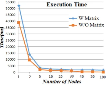
D. Scalability
The goal here is to determine the effects of the number of nodes in the system on the execution times. The dataset
contains 50,000 data points. Figure 6 shows the execution time against the number of nodes (x axis is in log2) in the system. As one can see, DDC-DBSCAN took only few seconds (including the matrix computation’s time) to cluster
50,000 data points in a distributed system that contains up to 100 nodes, the algorithm took even less time when we exclude the matrix computation’s time. Thus, the algorithm can comfortably handle high-dimensional data because of its low complexity.
Fig. 6: Scalability Experiments.
VI. CONCLUSION
In this paper, we proposed an efficient and flexible dis-tributed clustering framework that can work with existing data mining algorithms. The framework has been tested on spatial datsests using the K-Means and DBSCAN algorithms. The dis-tributed clustering approach is moreover dynamic, for spatial datasets, as it does not need to give the number of correct clus-ters in advance (as an input parameter). This basically solves one of major shortcomings of K-Means or DBSCAN. The proposed Distributed Dynamic Clustering (DDC) approach has two main phases: the fully parallel phase where each node of the system calculates its own local clusters based on its portion of the entire dataset. There is no communications during this phase, it takes full advantage of task parallelism paradigm. The second phase is also distributed, but it generates some communications between the nodes. However, the overhead due these communications has minimised by using a new concept of cluster representatives. Each cluster is represented by its contour and its density, which count for about 1% of cluster size in general. This DDC framework can easily be implemented using MapReduce mechanism.
Note that, as the first phase is fully parallel, each node can use its own clustering algorithm that suits well its local dataset. However, the quality of the DDC final results depends heavily on the local clustering used during the first phase. Therefore, the issue of exploring the original dataset before choosing local clustering algorithms remains the key hurdle of all the data mining techniques.
The DDC approach was tested using various benchmarks. The benchmarks were chosen in such a way to reflect all the difficulties of clusters extraction. These difficulties include the shapes of the clusters (convex and non-convex), the data vol-ume, and the computational complexity. Experimental results showed that the approach is very efficient and can deal with various situations (various shapes, densities, size, etc.).
As future work, we will study in more details the approach scalability on very large datasets, and we will explore other models for combining neighbouring clusters such as dynamic tree-based searching and merging topology on large scale platforms [47], [48], [49]. We will extend the framework to non-spatial datasets by using Knowledge Map [50] for example. We will also look at the problem of the data and communications reduction during phase two.
ACKNOWLEDGMENT
The research work is conducted in the Insight Centre for Data Analytics, which is supported by Science Foundation Ireland under Grant Number SFI/12/RC/2289.
REFERENCES
[1] J. Han and M. Kamber,Data Mining: Concepts and Techniques, 2nd ed. Morgan Kaufmann Publisher, 2006.
[2] L. Aouad, N.-A. Le-Khac, and M.-T. Kechadi, “weight clustering technique for distributed data mining applications,”LNCS on advances in data mining – theoretical aspects and applications, vol. 4597, pp. 120–134, 2007.
[3] L.Aouad, N.-A. Le-Khac, and M.-T. Kechadi, “Grid-based approaches for distributed data mining applications,” Journal of Algorithms & Computational Technology, vol. 3, no. 4, pp. 517–534, 2009. [4] L. Aouad, N.-A. Le-Khac, and M.-T. Kechadi, “Performance study
of distributed apriori-like frequent itemsets mining,” Knowledge and Information Systems, vol. 23, no. 1, pp. 55–72, 2010.
[5] M. Whelan, N.-A. L. Khac, and M.-T. Kechadi, “Performance eval-uation of a density-based clustering method for reducing very large spatio-temporal dataset,” in in Proc. of International Conference on Information and Knowledge Engineering, July 18-21 2011.
[6] M. Bertolotto, S. Di Martino, F. Ferrucci, and M.-T. Kechadi, “Towards a framework for mining and analysing spatio-temporal datasets,” Inter-national Journal of Geographical Information Science, vol. 21, no. 8, pp. 895–906, 2007.
[7] N.-A. Le-Khac, L. Aouad, and M.-T. Kechadi, “Knowledge map layer for distributed data mining,”Journal of ISAST Transactions on Intelli-gent Systems, vol. 1, no. 1, 2008.
[8] P. Chan and S. Stolfo, “A comparative evaluation of voting and meta-learning on partitioned data,” in 12th International Conference on Machine Learning, 1995, pp. 90–98.
[9] C. Reeves, Modern heuristic techniques for combinatorial problems. John Wiley & Sons, Inc. New York, NY, USA, 1993.
[10] T. G. Dietterich, “An experimental comparison of three methods for constructing ensembles of decision trees: Bagging, boosting, and ran-domization,”Machine Learning, vol. 40, no. 2, pp. 139–157, 2000. [11] H. Kargupta and P. Chan,Advances in distributed and Parallel
Knowl-edge Discovery. MIT Press Cambridge, MA, USA, Oct. 2000, vol. 5. [12] J.-M. Adamo,Data mining for association rules and sequential pat-terns: sequential and parallel algorithms. Springer Science & Business Media, 2012.
[13] N.-A. Le-Khac, L. Aouad, and M.-T. Kechadi, “Performance study of distributed apriori-like frequent itemsets mining,” Knowledge and Information Systems, vol. 23, no. 1, pp. 55–72, 2010.
[14] N. A. Le Khac, L. M. Aouad, and M.-T. Kechadi, Emergent Web Intelligence: Advanced Semantic Technologies. London: Springer London, 2010, ch. Toward Distributed Knowledge Discovery onGrid Systems, pp. 213–243.
[15] E. Januzaj, H.-P. Kriegel, and M. Pfeifle, Advances in Database Technology - EDBT 2004: 9th International Conference on Extending Database Technology, Heraklion, Crete, Greece, March 14-18, 2004. Berlin, Heidelberg: Springer Berlin Heidelberg, 2004, ch. DBDC: Density Based Distributed Clustering, pp. 88–105.
[16] N. Le-Khac, L.Aouad., and M.-T. Kechadi,Data Management. Data, Data Everywhere: 24th British National Conference on Databases, BNCOD 24, Glasgow, UK, July 3-5, 2007. Berlin, Heidelberg: Springer Berlin Heidelberg, 2007, ch. A New Approach for Distributed Density Based Clustering on Grid Platform, pp. 247–258.
[17] L. Aouad, N.-A. L. Khac, and M.-T. Kechadi,Advances in Data Mining. Theoretical Aspects and Applications: 7th Industrial Conference (ICDM 2007), Leipzig, Germany, July 14-18, 2007. Proceedings. Berlin, Hei-delberg: Springer Berlin Heidelberg, 2007, ch. Lightweight Clustering Technique for Distributed Data Mining Applications, pp. 120–134. [18] J.-F. Laloux, N.-A. Le-Khac, and M.-T. Kechadi, “Efficient distributed
approach for density-based clustering,”Enabling Technologies: Infras-tructure for Collaborative Enterprises (WETICE), 20th IEEE Interna-tional Workshops, pp. 145–150, 27-29 June 2011.
[19] M. K. Jiawei Han, Data Mining: Concepts and Techniques, 2nd ed. Elsevier, Diane Cerra, San Francisco, CA 94111, 2006, ch. Introduction. [20] M. J. Zaki, Large-Scale Parallel Data Mining. Berlin, Heidelberg: Springer Berlin Heidelberg, 2000, ch. Parallel and Distributed Data Mining: An Introduction, pp. 1–23.
[21] S. Ghosh,Distributed systems: an algorithmic approach. CRC press, 2014.
[22] L. Aouad, N.-A. Le-Khac, and M.-T. Kechadi., “Image analysis plat-form for data management in the meteorological domain,” in 7th Industrial Conference, ICDM 2007, Leipzig, Germany, July 14-18, 2007. Proceedings, vol. 4597. Springer Berlin Heidelberg, 2007, pp. 120–134.
[23] X. Wu, X. Zhu, G. Q. Wu, and W. Ding, “Data mining with big data,” IEEE Transactions on Knowledge and Data Engineering, vol. 26, no. 1, pp. 97–107, 2014.
[24] L. Rokach, A. Schclar, and E. Itach, “Ensemble methods for multi-label classification,”Expert Systems with Applications, vol. 41, no. 16, pp. 7507 – 7523, 2014.
[25] R. K. Eric Bauer, “An empirical comparison of voting classification algorithms: Bagging, boosting, and variants,” springer Link:Machine Learning, vol. 36, pp. 105–139, 1999.
[26] M. L. Tian Zhang, Raghu Ramakrishnan, “Birch: An efficient data clus-tering method for very large databases,” inSIGMOD ’96 Proceedings of the 1996 ACM SIGMOD international conference on Management of data, vol. 25, 1996, pp. 103–114.
[27] P. J. F. A. K. Jain, M. N. Murty, “Data clustering: a review,” ACM Computing Surveys (CSUR), vol. 31, pp. 264–323, 1999.
[28] I. Dhillon and D. Modha, “A data-clustering algorithm on distributed memory multiprocessor,” inlarge-Scale Parallel Data Mining, Work-shop on Large-Scale Parallel KDD Systems, SIGKDD. Springer-Verlag London, UK, 1999, pp. 245–260.
[29] M. Ester, H.-P. Kriegel, J. Sander, and X. Xu, “A density-based algorithm for discovering clusters in large spatial databases with noise.” inKdd, vol. 96, no. 34, 1996, pp. 226–231.
[30] A. Garg, A. Mangla, V. Bhatnagar, and N. Gupta, “Pbirch: A scalable parallel clustering algorithm for incremental data,”10th Int’l. Sympo-sium on Database Engineering and Applications (IDEAS-06), pp. 315– 316, 2006.
[31] H.Geng, Omaha, and X. Deng, “A new clustering algorithm using message passing and its applications in analyzing microarray data,” in ICMLA ’05 Proc. of the 4th Int’l. Conf. on Machine Learning and Applications. IEEE, 15-17 December 2005, p. 145150.
[32] I. D. Dhillon and D. S. Modha, “A data-clustering algorithm on distributed memory multiprocessors,” in Large-Scale Parallel Data Mining. Springer Berlin Heidelberg, 2000, pp. 245–260.
[33] X. Xu, J. Jger, and H.-P. Kriegel, “A fast parallel clustering algorithm for large spatial databases,” Data Mining and Knowledge Discovery archive, vol. 3, pp. 263–290, September 1999.
[34] N.-A. Le-Khac, M. Bue, M. Whelan, and M-T.Kechadi, “A knowl-edgebased data reduction for very large spatio-temporal datasets,”
International Conference on Advanced Data Mining and Applications, (ADMA2010), 19-21 November 2010.
[35] M. Fadilia, M. Melkemib, and A. ElMoataza, Pattern Recognition Letters:Non-convex onion-peeling using a shape hull algorithm. EL-SEVIER, 15 October 2004, vol. 24.
[36] A. Chaudhuri, B. Chaudhuri, and S. Parui, “A novel approach to computation of the shape of a dot pattern and extraction of its perceptual border,”Computer vision and Image Understranding, vol. 68, pp. 257– 275, 03 December 1997.
[37] M. Melkemi and M. Djebali, “Computing the shape of a planar points set,”Elsevier Science, vol. 33, p. 14231436, 9 September 2000. [38] H. Edelsbrunner, D. G. Kirkpatrick, and R. Seidel, “On the shape of a
set of points in the plane,”Information Theory, IEEE Transactions on, vol. 29, no. 4, pp. 551–559, 1983.
[39] A. Moreira and M. Y. Santos, “Concave hull: A k-nearest neighbours approach for the computation of the region occupied by a set of points,” inInt’l. Conf. on Computer Graphics Theory and Applications (GRAPP-2007), Barcelona, Spain, 8-11 March 2007, pp. 61–68.
[40] M. Duckhama, L. Kulikb, M. Worboysc, and A. Galtond, “Efficient generation of simple polygons for characterizing the shape of a set of points in the plane,”Elsevier Science Inc. New York, NY, USA, vol. 41, pp. 3224–3236, 15 March 2008.
[41] M. Bendechache and M.-T. Kechadi, “Distributed clustering algorithm for spatial data mining,” inIn Proc of the 2nd IEEE Int’l. Conf. on Spatial Data Mining and Geographical Knowledge Services (ICSDM-2015), Fuzhou, China, 2015, pp. 60–65.
[42] M.Ester, H. Kriegel, J. Sander, and X. Xu, “A density-based algorithm for discovering clusters in large spatial databases with noise,”In 2nd Int. Conf., Knowledge Discovery and Data Mining (KDD 96), 1996. [43] T. Kanungo, S. Jose, D. M. Mount, N. S. Netanyahu, and C. D. Piatko,
“An efficient k-means clustering algorithm: Analysis and implementa-tion,”IEEE Transactions on pattern analysis and machine intelligence, vol. 24, July 2002.
[44] T. Zhang, R. Ramakrishnan, and M. Livny, “Birch: An efficient data clustering method for very large databases,” inSIGMOD-96 Proceed-ings of the 1996 ACM SIGMOD international conference on Manage-ment of data, vol. 25. ACM New York, USA, 1996, pp. 103–114. [45] W. Wang, J. Yang, and R. R. Muntz, “Sting: A statistical information
grid approach to spatial data mining,” inIn Proc. of the 23rd Int’l. Conf. on Very Large Data Bases, ser. VLDB ’97. San Francisco, CA, USA: Morgan Kaufmann Publishers Inc., 1997, pp. 186–195.
[46] S. Guha, R. Rastogi, and K. Shim, “Cure: An efficient clustering algorithm for large databases,” inInformation Systems, vol. 26. Elsevier Science Ltd. Oxford, UK, 17 November 2001, pp. 35–58.
[47] B. Hudzia, M.-T. Kechadi, and A. Ottewill, “Treep: A tree-based p2p network architecture,” in2005 IEEE International Conference on Cluster Computing. IEEE, 2005, pp. 1–15.
[48] I. K. Savvas and M.-T. Kechadi, “Dynamic task scheduling in com-puting cluster environments,” in Parallel and Distributed Computing, 2004. Third International Symposium on/Algorithms, Models and Tools for Parallel Computing on Heterogeneous Networks, 2004. Third Inter-national Workshop on. IEEE, 2004, pp. 372–379.
[49] N.-A. Le-Khac, S. Markos, M. O’Neill, A. Brabazon, and M.-T. Kechadi, “An efficient search tool for an anti-money laundering appli-cation of an multi-national bank’s dataset.” inIKE, 2009, pp. 151–157. [50] N.-A. Le-Khac, L. Aouad, and M.-T. Kechadi, “Knowledge map: Toward a new approach supporting the knowledge management in distributed data mining,” inAutonomic and Autonomous Systems, 2007. ICAS07. Third International Conference on. IEEE, 2007, pp. 67–67.