IN
2D
AND
3D V
ECTOR
F
IELDS
Dissertation
zur Erlangung des akademischen Grades
Doktoringenieur (Dr.-Ing.)
angenommen durch die Fakultät für Informatik
der Otto-von-Guericke-Universität Magdeburg
von Dipl.-Inf. Tino Weinkauf
geboren am 31. Oktober 1974 in Rostock
Gutachter:
Prof. Dr. Holger Theisel
Prof. Dr. Thomas Ertl
Prof. Alex Pang, Ph.D.
Wenn zwei Menschen über eine lange Zeit an verschiedenen Orten leben und sowohl ihre Freundschaft erhalten als auch erfolgreich gemeinsam arbeiten wollen, dann müs-sen sie sich blind verstehen. Mit meinem Freund und Doktorvater Holger Theisel kann ich das. Die letzten Jahre haben nicht einfach nur Spaß gemacht, sondern sie haben mich definiert. Deine Art zu forschen, nehme ich mir als Vorbild.
Meinem Gutachter Thomas Ertl möchte ich herzlich danken für sein tiefgehendes und sorgfältiges Gutachten dieser Arbeit.
Alex Pang reviewed this thesis and I am deeply grateful for this. It was great that you could make it to the disputation.
Meinem Freund und Kollegen Jan Sahner bin ich sehr dankbar für die wunderbare Zusammenarbeit bei der Forschung und beim Schreiben von Anträgen. Deine positive Grundeinstellung hat unsere Arbeit geprägt und alles ein bisschen leichter gemacht, selbst die quälenden Dinge.
Hans-Christian Hege gilt mein besonderer Dank. Seine Unterstützung über all die Jahre meiner Arbeit am ZIB ist einzigartig. Die Arbeitsatmosphäre am ZIB ist groß-artig und alle Kollegen sind mir sehr ans Herz gewachsen. Das hat sich nicht zuletzt auch positiv auf diese Arbeit ausgewirkt. Insbesondere möchte ich meinen Studenten Jan Reininghaus, Nathalie Teuber und Norbert Lindow für ihre Unterstützung danken. Man kann eine aussagekräftige Visualisierung nur dann produzieren, wenn man den Hintergrund versteht. Bernd R. Noack hat sich viel Zeit genommen, um mir dieses Verständnis in vielen langen und schönen Gesprächen zu vermitteln. Bernd, ich danke Dir. Desweiteren gilt mein Dank auch den anderen Mitarbeitern des Instituts für Strö-mungsmechanik und Technische Akustik der TU Berlin, die mir immer hilfreich zur Seite standen.
Meine Eltern haben mich immer auf meinem Weg begleitet. Eure Energie hat mir viel Kraft gegeben, eure Geduld die Ausdauer. Ich danke Euch.
Mit wenigen Menschen schwingt man im Takt. Mit Dir, Wenke, ist es eine Sinfonie.
Die Arbeit an meiner Dissertation hat viel Kraft und Zeit erfordert, und ich bin sehr glücklich darüber, dieses aufbringen zu können. Mit Eurer Hilfe.
Tino Weinkauf 23. April 2008
Analyzing large and high-dimensional flow data sets is a non-trivial task and favorably carried out using sophisticated tools which allow to concentrate on the most relevant information and to automate the analysis. These goals can be achieved using topolog-ical methods, which foster target-oriented studies of the most important flow features. They have a variety of applications which ranges from a skeletal representation of the overall flow behavior to a detailed analysis of vortex structures.
This thesis presents novel algorithms and approaches for the extraction, tracking and visualization of topological structures of vector fields. The new concept of con-nectors is introduced which allows visually simplified representations of topological skeletons of complex 3D vector fields. The first visualization technique for 3D higher order critical points and the corresponding classification are presented. Based on this theory, two novel applications for the topological simplification and construction of 3D vector fields have been developed. Furthermore, the first generic approach to feature extraction is presented, which allows to extract and track a rich variety of geometri-cally defined, local and global features evolving in scalar and vector fields. The use of generic concepts and grid independent algorithms aims at a broad applicability of the extraction methods while alleviating the implementational expenses. Further contribu-tions include the first topology-based visualization approach for two-parameter-depen-dent 2D vector fields and a thorough study of vortex structures. The usefulness of the newly developed methods is shown by applying them to analyze a number of data sets. The work presented in this thesis has been published in peer-reviewed international conference proceedings, journals, and books.
Zusammenfassung
Die Analyse von großen und hochdimensionalen Strömungsdaten stellt eine Herausfor-derung dar, bei der sich die Verwendung von automatisierbaren Werkzeugen bewährt hat, die eine Konzentration auf die wesentlichen Informationen erlauben. Topologische Analyseverfahren erlauben eine zielorientierte Untersuchung der relevantesten Strö-mungsmerkmale und lassen sich vielfältig anwenden, von der skelettartigen Darstel-lung des Strömungsverhaltens bis hin zur detaillierten Analyse von Wirbelstrukturen.
Diese Dissertation stellt neue Algorithmen und Ansätze zur Extraktion, zeitlichen Verfolgung und Visualisierung von topologischen Strukturen in Vektorfeldern vor. Zur vereinfachten Darstellung topologischer Skelette von komplexen 3D Vektorfeldern wur-de das neue Konzept wur-der Konnektoren entwickelt. Die erste Visualisierungstechnik für 3D kritische Punkte höherer Ordnung und die zugehörige Klassifikation werden vor-gestellt. Auf Basis dieser Theorie wurden zwei neue Anwendungen zur topologischen Simplifizierung und Konstruktion von 3D Vektorfeldern entwickelt. Desweiteren wird der erste generische Ansatz zur Extraktion von Merkmalen vorgestellt, der es erlaubt, eine Vielzahl von geometrisch definierten, lokalen und globalen Merkmalen in Skalar-und Vektorfeldern zu extrahieren Skalar-und zeitlich zu verfolgen. Die Verwendung gene-rischer Konzepte und gitterunabhängiger Algorithmen zielt auf eine breite Anwend-barkeit der Methoden bei gleichzeitig vergleichsweise geringem Implementationsauf-wand. Zu den weiteren Beiträgen der Arbeit gehören der erste topologiebasierte Ansatz zur Visualisierung von zwei-parameterabhängigen 2D Vektorfeldern und eine umfas-sende Studie von Wirbelstrukturen. Die Nützlichkeit der Methoden wird anhand der Analyse verschiedener Datensätze gezeigt.
Die in dieser Dissertation vorgestellten Arbeiten wurden in begutachteten interna-tionalen Konferenzbänden, Zeitschriften und Büchern veröffentlicht.
1 Introduction 7
1.1 Related Work . . . 11
2 Theory 17 2.1 Notations and Definitions . . . 17
2.1.1 Basic Notations . . . 17
2.1.2 Characteristic Curves of Vector Fields . . . 18
2.1.3 Derived Measures of Vector Fields . . . 21
2.2 Parameter-Independent Topology . . . 22
2.2.1 Critical Points . . . 22
2.2.2 Boundary Switch Points and Curves . . . 25
2.2.3 Separatrices . . . 27
2.2.4 Saddle Connectors . . . 28
2.2.5 Boundary Switch Connectors . . . 31
2.2.6 Closed Stream Lines . . . 32
2.3 Parameter-Dependent Topology . . . 33
2.3.1 Bifurcations of One-Parameter-Dependent Vector Fields . . . 34
2.3.2 Two-Parameter-Dependent Topology . . . 36
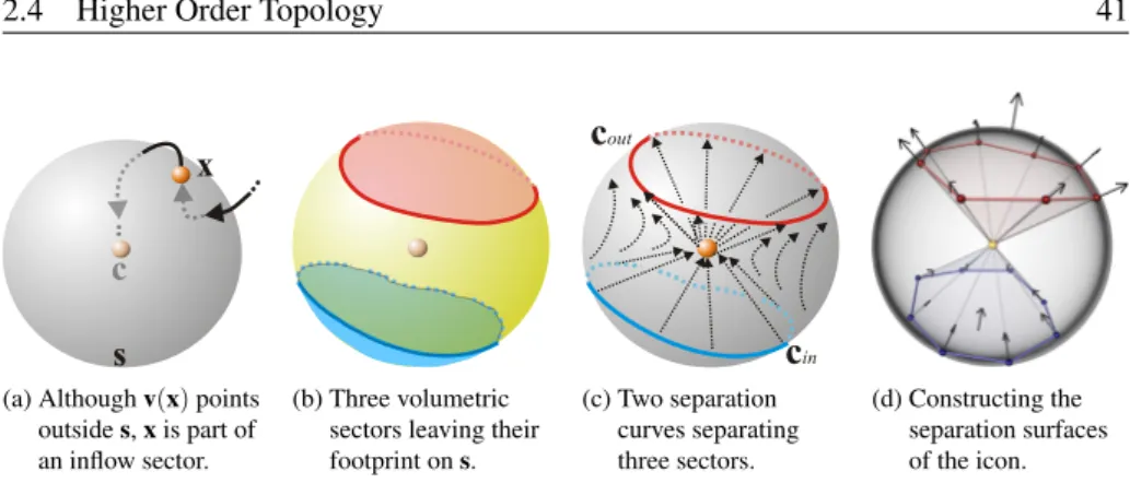
2.4 Higher Order Topology . . . 38
2.4.1 2D Vector Fields . . . 40
2.4.2 3D Vector Fields . . . 41
3 Concepts and Basic Algorithms for Extraction 43 3.1 Feature Flow Fields . . . 44
3.1.1 Feature Flow Fields in Out-Of-Core Settings . . . 46
3.1.2 Feature Flow Fields and the Parallel Vectors Operator . . . 50
3.2 Connectors . . . 52
3.3 Unified Feature Extraction Architecture . . . 53
3.3.1 Finding Zeros . . . 55
3.3.2 Integrating Stream Objects . . . 55
3.3.3 Intersecting Stream Objects . . . 57
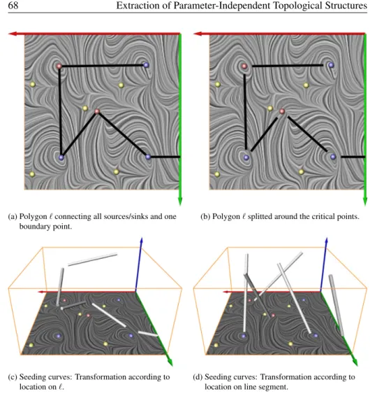
4 Extraction of Parameter-Independent Topological Structures 61 4.1 Features induced by Critical Points . . . 61
4.2 Features induced by the Boundary . . . 63
4.3 Closed Stream Lines . . . 65
5.1.1 Tracking Critical Points . . . 76
5.1.2 Global Bifurcations . . . 80
5.2 Applications . . . 85
5.3 Two-Parameter-Dependent Topology . . . 89
5.3.1 Tracking Fold Bifurcations . . . 90
5.3.2 Fold-fold Bifurcations . . . 91
5.3.3 Tracking Hopf Bifurcations . . . 94
5.4 Applications . . . 96
6 Extraction of Higher Order Topological Structures and Topological Sim-plification 101 6.1 Extracting the Sectors Around a Critical Point . . . 102
6.1.1 Auxiliary vector fields . . . 102
6.1.2 F-classification of a single point ons. . . 104
6.1.3 F-classification of all points ons . . . 106
6.1.4 A complete system of 2D topological substructures . . . 107
6.1.5 Obtaining a minimal skeleton . . . 109
6.2 Applications . . . 111
7 Further Applications of Topological Concepts and Methods 115 7.1 Construction of Higher Order 3D Vector Fields . . . 115
7.1.1 Why Modeling Vector Fields? . . . 116
7.1.2 Modeling the Topological Skeleton . . . 117
7.1.3 Construction of the Vector Field . . . 120
7.1.4 Examples . . . 123
7.2 Vortex Core Lines . . . 126
7.2.1 Cores of Swirling Motion . . . 127
7.2.2 Galilean Invariant Vortex Core Lines . . . 136
7.2.3 Vortex and Strain Skeletons . . . 142
7.3 Steering of other Visualization Techniques . . . 146
8 Discussion 151 8.1 Topology of other Characteristic Curves . . . 151
8.2 Noise and Derivatives . . . 152
8.3 Turbulent Flows . . . 153
8.4 Topological Complexity of 2D and 3D Vector Fields . . . 154
8.4.1 Counting the Number of Sectors . . . 154
8.4.2 Interpretation of Sector Counting . . . 160
9 Conclusion and Future Work 163
Bibliography 166
List of Figures 183
Introduction
Computing power increases constantly. While the fastest supercomputer in 1993 had a performance of 59.7 GFlop/s, the fastest installation in 2007 reached 280.6 TFlop/s [MSDS]. This is an increase by a factor of 4700. As of this writing, the petascale era is already approaching. Along with the computing power, the size and complexity of simulation results is increasing as well. In many cases the simulated data sets are at least four-dimensional, e.g. with three spatial dimensions and time. In some cases even higher-dimensional data sets are produced by considering additional parameters.
Due to the sheer size of the data sets alone, it is favorable if not necessary to au-tomate at least parts of the analysis. A way to achieve this is by extracting features.
Afeature– as used in this thesis – is a mathematically well-defined, geometric object
(point, line, surface,. . .) with its definition and interpretation depending on the under-lying application, but usually it represents important structures (e.g. vortex, stagnation point) or changes to such structures (events, bifurcations). An automated extraction of features aids an analysis in a number of ways:
• reduction of information
The human brain has the ability to grasp primarily three dimensions and the current hardware has only limited capabilities of displaying them. Hence, only parts of the massive and complex simulation results can be visualized at once. Feature extraction reduces the amount of data to a small set of geometric objects. Furthermore, a quantification of the extracted features allows to build up a feature hierarchy leading to even further simplified representations by e.g. filtering out the less important features.
• target-oriented study
Feature extraction is used to automatically find interesting parts in the data, where e.g. certain structural changes occur. This can guide the user in the manual exploration of a data set. It allows to concentrate on certain aspects of the data – leading to a target-oriented, application-dependent study of the most important structures of a data set.
• shifting the analysis to the supercomputer
In some cases it is preferable to analyze the data on the supercomputer along the simulation: for example, if the data set is too large to be efficiently handled by commodity hardware, or if the analysis results have some influence on the
(a) Stream lines. (b) Sources (red), sinks (blue), and saddles (yellow). (c) Separation lines emanating from saddles. (d) Sectors of different flow behavior.
Figure 1.1: Topology of a simple 2D vector field.
simulation itself (e.g. simulation steering). Feature extraction is easily automated and therefore, it is perfectly fitted for batch jobs on supercomputers.
• interactive visualization
The resulting feature set is usually small enough to be handled and displayed interactively with commodity hardware.
• more objective analysis
In contrast to most other visualization methods, feature extraction techniques usually depend on less parameters or even no parameters at all. Hence, the in-terpretation of the results depends less on a user-defined parametrization (e.g. isovalue, transfer function).
• faster analysis
The time needed by the user is reduced since parts of the analysis are automated and the manual part is interactive.
This thesis is concerned with the feature-based analysis of vector fields, with the main focus on flow fields which play a vital role in many areas. Examples are burn-ing chambers, turbomachinery and aircraft design in industry as well as blood flow in medicine.
The analysis is based on the extraction and examination of topological structures of vector fields. Topology is a well-researched field of mathematics. It allows to condense a data set to its structural skeleton. For vector fields, this means to segment the domain into regions of different flow behavior. Consider a simple 2D vector field as shown in figure 1.1a. A topological analysis always starts with the extraction of so-called critical points which are the zeros of the vector field. As it can be observed in figure 1.1b there are different flow patterns around critical points which allow to classify them into sources, sinks, and saddles. While the flow behavior around sources and sinks is uniformly either outflow or inflow, the flow around saddles is a mixture of both. Certain stream lines around saddles can be found which separate these different areas. They are called separation lines (figure 1.1c). This leads to a complete segmentation of the domain into regions of different flow behavior as highlighted in figure 1.1d.
Topology can be used in a number of ways to foster the analysis of flows. For example, the topology of the velocity field of a flow can be seen as a condensed repre-sentation of the stream lines and may therefore serve as a skeletal, simplified represen-tation of the flow. However, such an analysis depends on the reference frame and may therefore be not applicable in all situations. As another application, the topological
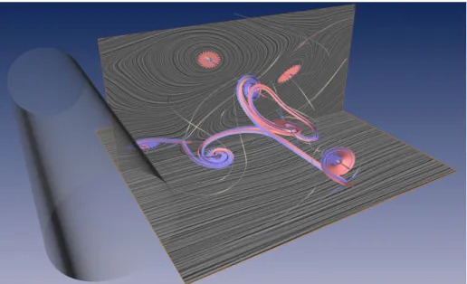
(a) The line integral convolution method depicts the vortices, but is incapable of measuring properties like their velocity.
(b) A feature-based analysis extracts the cores of the vortices as distinct geometric objects (lines) and tracks them over time (surfaces).
Figure 1.2: Difference between visual and feature-based analysis at a flow behind a cylinder. Data courtesy of Bernd R. Noack (TU Berlin) and Gerd Mutschke (FZ Rossendorf).
structures of certain derived vector fields describe centers of high strain or vortex ac-tivity – leading to a Galilean invariant analysis of important flow processes like mixing. In the following we give two examples of how flows can be analyzed using the theory and tools developed in this thesis.
A feature-based analysis gives rise to new possibilities in comparison to other visu-alization techniques. Consider the flow behind a cylinder as shown in figure 1.2. The so-called von Kármán vortex street develops behind the cylinder and is clearly depicted by the line integral convolution method shown in figure 1.2a. Using an animation, the temporal movement of these vortices can be depicted by this method as well. However, it is incapable ofdistinguishingbetween different vortices andmeasuringtheir path, velocity, or life time. The feature-based vortex analysis shown in figure 1.2b allows this since the vortices have been extracted as distinct geometric objects. Furthermore, it is possible to quantify these objects by means of importance or strength, and to filter accordingly.
Figure 1.3 shows an example where a topology-based analysis has been success-fully applied to explain the impact of an active flow control technique at an airfoil. The flow around an airfoil is subject to large efforts in order to increase the desired lift and to reduce the parasitic drag. In this example, these performance enhancements are achieved by controlling the flow separation at the rear flap using periodic air injection (figure 1.3a). The uncovering of the underlying physics was a necessary step in order to choose optimal values for frequency, intensity, and angle of the injection. Based on this, the lift could be raised by 11.2%. The vortex structures have been extracted as topological separatrices of the pressure gradient and denote lines of minimal pressure. Figure 1.3c shows parts of the topological skeleton of the pressure gradient. A quan-tification of the separation lines based on pressure and a subsequent filtering of weak vortices has been applied. The result is shown in figures 1.3d–f where the impact of the frequency of air injection onto the vortex structures can be studied. Note that this is a five-dimensional data set consisting of three spatial dimensions, time, and the param-eter dimension. Raising the frequency causes a reduction of the lower vortex, which
(a) Periodic excitation by suction and blowing at the rear flap.
(b) Colormap used to indicate flow pressure and vortex strength.
(c) A subset of the topological skeleton of the pressure gradient denotes minimal pressure, i.e., vortex cores.F+=2.0.
(d) Vortex structures of the unexcited flow.
(e) Vortex structures of the optimally excited flow (F+=0.6). Gain of lift: 11.2%.
(f) Vortex structures of the high-frequency excited flow (F+=2.0). Gain of lift: 6.1%. Figure 1.3: A topology-based vortex analysis of the flow around an airfoil elucidates the impact of an active flow control technique and explains why a high-frequency ex-citation leads to a smaller gain of lift. Data courtesy of Bert Günther (TU Berlin).
is a necessary condition for gaining lift. However, higher frequencies (F+>0.6) are not beneficial to the lift. Using a visual comparison of the vortex structures at different frequencies, we found that new vortex structures are induced by the air injection itself. This has a negative effect on the pressure ratio and consequently on the lift. Especially at higher frequencies, the excitation dominates the natural flow structures and induces long-living, almost two-dimensional vortices in fast succession at the top of the rear flap (figure 1.3f). In contrast to this, the induced vortices atF+=0.6 dissolve quickly and therefore, they are less influential. Our topology-based analysis technique of the vortex structures contributed to the physical understanding of the flow structures and was a substantial part of the optimal choice of parameters.
In chapter 2 we discuss the theoretical background needed for this thesis and add the notions of saddle connectors and boundary switch connectors to the body of theory. Furthermore, a geometrical description of the flow behavior around higher order critical points is introduced.
The main part of this thesis, chapters 3 – 6, deals with the extraction of topological structures. The foundation of most extraction techniques developed in the course of this thesis is presented in chapter 3: the so-called Unified Feature Extraction Architecture defines a small but comprehensive set of algorithms and concepts, which allows to
extract and track a variety of topological and other features. It is a major contribution of this thesis and the first generic approach to feature extraction treating local and global features.
Based on this architecture we formulate most of the extraction techniques in the following chapters, which deal with first order topological structures of steady vector fields (chapter 4), time-dependent and two-parameter-dependent vector fields (chapter 5), or higher order topological structures (chapter 6). Major contributions in these chapters are the extraction of connectors, several novel algorithms for the treatment of global bifurcations, the first topology-based visualization approach for two-parameter-dependent vector fields, and the first topological simplification method for 3D vector fields. Along with the development of these methods we show their usefulness by applying them to analyze a number of data sets.
Further applications of topological concepts and methods are presented in chapter 7. We show how to construct 3D vector fields from a given topological description, or how the results of a topological analysis can be used to steer other visualization techniques. The main part of this chapter, however, is devoted to the treatment of vortex core lines. We show how these lines can be extracted and tracked using the methods developed in previous chapters. Furthermore, we give a unified notation of cores of swirling motion, present a novel way of describing vortex core lines as extremum lines, and link the fields of topology and vortex analysis by showing how vortex core lines can be described as topological separatrices of a derived vector field.
We discuss the applicability of topological methods in chapter 8. Among other things, we comment on noise sensitivity and turbulent flows, and we study the topolog-ical complexity of 2D and 3D vector fields. Chapter 9 draws conclusions and gives an outlook to future work.
The work presented in this thesis has been published in peer-reviewed international conference proceedings, journals, and books:
• Extracting and tracking topological structures: [TWHS03, WTHS04a, TWHS04a, TWHS04b, TWHS05, WTHS06]
• Simplification and construction: [WTHS04b, WTS+05]
• Concepts and theoretical foundations: [WTHS07, TWHS07, WST+07, TRW08]
• Vortex analysis: [SWH05a, TSW+05, SWTH07, WSTH07]
• Applications: [WHN+02, WHN+03, HWPH04, WNC+04, HWPH05, PWS+06, GTP+07]
1.1
Related Work
In the following we give an overview of related work. We restrict the discussion to the field of flow visualization with a major focus on topology-based analysis. Following the approach of Post et al. [PVH+02], we subdivide the field of flow visualization into
direct,integration-based, andfeature-basedmethods.
Direct flow visualization methods map the data to an image without involved com-putations. Examples are color coding [SRBE99], volume rendering [CMBC93, EYSK94, RLMO03], arrow plots [KH91, BP96], or combinations thereof [KML99].
The class of integration-based methods can be subdivided intotexture-based and
geometry-basedtechniques. All these methods employ numerical integration schemes
which introduce a certain amount of uncertainty due to integration errors. Lodha et al. [LPSW96] and Pang et al. [PWL97] provide a number of solutions for depicting this uncertainty.
Van Wijk introduced the first texture-based method called spot noise [vW91], which has later been extended to include magnitude information [dLvW95]. Cabral and Lee-dom [CL93] developed the line integral convolution method (LIC), where a noise tex-ture is filtered along the stream lines of the vector field. This yields dense represen-tations. Stalling and Hege [SH95a] significantly lowered the computation times for LIC by exploiting coherence along the stream lines. Later improvements include di-rectional clues [WGP97, WLG97], animation [SK97], GPU-accelerated implementa-tions [HWSE99], extension to surfaces [BSH96, SH97, MKFI97] and to 3D [IG97, RSHTE99]. A comparison between LIC and spot noise can be found in [dLvL98].
Some work has been done on the field of texture advection for the visualization of time-dependent vector fields: Moving Textures by Max and Becker [MB95], the Lagrangian-Eulerian Advection method (LEA) by Jobard et al. [JEH02], and Image Based Flow Visualization (IBFV) by van Wijk [vW02] to name a few. The latter has been extended to 3D surfaces [vW03, LJH03] and volumes [TvW03]. Weiskopf et al. [WEE03] present a generic framework for texture-based visualization of 2D unsteady flows. A thorough overview of texture-based methods can be found in [LHD+04].
Geometry-based methods visualize the characteristic curves of flow fields (see also section 2.1.2) or parts thereof as points, lines, surfaces, or volumes. Kenwright and Lane [KL96] present a particle tracer for time-dependent flows which gains its inter-activity from tetrahedral decomposition. Two approaches to accelerate particle trac-ing on sparse grids are given by Teitzel and Ertl [TE99]. Krüger et al. [KKKW05] present a highly interactive particle system implemented on the GPU. Line-type struc-tures such as stream or path lines can be visualized using the illumination method of Zöckler et al. [ZSH96], which allows a fast cylindrical shading using a texture lookup. Mallo et al. [MPSS05] improved the method by incorporating a different diffuse reflection term. A number of methods have been proposed to distribute the seeding points [ZSH96, VKP00, YKP05], or to distribute the stream lines themselves [TB96, JL97, MAD05]. The computation of stream surfaces can be reduced to the integration of a finite number of adjacent stream lines and appropriate triangulation between them [Hul92, Sta98, GTS+04a]. Implicit stream surfaces are computed by [vW93]. Krauskopf et al. [KOD+05] give an overview of different methods for com-puting stream surfaces. Löffelmann et al. [LMG97] propose the concept of stream arrows to enhance the visualization of stream surfaces by cutting away arrow-like ar-eas encoding flow direction or divergence. Similarly to stream surfaces, stream vol-umes can be computed by a proper tetrahedrization between adjacent stream lines as proposed by Max et al. [MBC93]. An appropriate projection of the tetrahedra yields smoke-like images. An extension to unsteady flows is given by Becker et al. [BML95]. A number of further geometry-based approaches have been derived from the stan-dard set of stream objects to encode additional information: examples are stream rib-bons, streamtubes, and streamballs, see [PVH+02].
Verma et al. [VKP99] presented a method to compare texture-based and geometry-based methods by mapping between a LIC and a stream line visualization – allowing a smooth transition.
Feature-based methods aim at presenting the most important parts of a data set at a high level of abstraction. The definition of importance depends on the application.
Among the features of interest are topological structures, vortices, as well as other features such as attachment and detachment lines or shock waves.
Topology in general is well-understood and thorough treatments can be found in [AS92, Bak91, GH86, Asi93, FG82].
Topological methods have been introduced as a visualization tool by Helman and Hesselink in their seminal work [HH89], where first order critical points are classified by an eigenvalue/eigenvector analysis of the Jacobian matrix, and separatrices starting from saddle points and from attachment and detachment points at no-slip boundaries are considered. This work has later been extended to 3D by the same authors [HH91]. Globus et al. [GLL91] present a system for visualizing the topological skeleton of 3D vector fields using icons and separation curves.
Since then a considerable amount of research has been done to extract, analyze, modify and visualize the topology of vector fields.
Several approaches can be used to extract critical points. In piecewise linear fields, the zeros can be computed explicitly. In more general settings, one might use a Newton-Raphson approach. An octree-like method is presented by Mann et al. [MR02]: they compute the index of each cell and a non-zero index triggers a recursive subdivision. An approach specifically designed for electric fields defined by a set of point charges has been presented by Max et al. [MW07]. Trotts et al. [TKH00] introduce the notion of critical points at infinity to find new separatrices. The curvature of stream lines in the proximity of critical points has been studied by Theisel and Weinkauf [The95, WT02] for 2D and 3D vector fields.
Regions of different flow behavior on the boundary of 2D vector fields as well as the corresponding separatrices have been considered by de Leeuw and van Liere [dLvL99a] and Scheuermann et al. [SHJK00].
Another type of separatrices are closed stream lines. A first approach to detecting closed stream lines was given by Wischgoll et al. [WS01] which uses the underlying grid structure of a piecewise linear vector field: each grid cell is analyzed concerning the re-entering behavior of the stream lines starting at its boundaries. Closed stream lines in 3D vector fields are discussed in [Asi93, PS07].
A thorough study of higher order critical points, i.e., critical points with a pos-sibly vanishing Jacobian, in 2D vector fields has been given by Firby and Gardiner [FG82]. Li et al. [LVRL06] discuss how to represent these points on triangular sur-faces using a carefully chosen triangulation and interpolation. Scheuermann et al. [SHK+97, SKMR98] give visualization approaches for planar flows.
For parameter-dependent vector fields, one aims at capturing the evolution of the topological structures. An important class of such fields are time-dependent flows. A common way of tracking the evolution is to extract the features in each time step and establish a correspondence afterwards based on Euclidean distance and feature attributes.
Tricoche et al. [TSH01b, TWSH02] track the location of critical points over time and detect local bifurcations like fold bifurcations and Hopf bifurcations. This ap-proach works on a piecewise linear 2D vector field and computes and connects the crit-ical points on the faces of a prism cell structure, which is constructed from the under-lying triangular grid. An extension to 3D has been given by Garth et al. [GTS04b] to-gether with a novel plot-like depiction of the critical points. Wischgoll et al. [WSH01] track closed stream lines over time by applying a contouring&connecting-like ap-proach: at each time step closed stream lines are detected independently of each other, then the corresponding lines in adjacent time steps are connected.
A grid-independent solution to feature tracking has been given by Theisel and Sei-del [TS03]. The basic idea is to track features of a time-dependent vector field by means of a stream line integration in a derived vector field – the so-called Feature Flow Field. This has been applied in [TS03] to track critical points. A number of further applications have been developed since then, see section 3.1 for an overview. A com-parable approach to tracking critical points in scale space is given by Klein and Ertl [KE07].
Some work has been done to measure the distance of vector fields by means of topology. This generally means to detect and match the critical points of two vector fields: for each critical point in the first vector field a corresponding critical point in the second vector field has to be found, and vice versa. Then the distances between all cor-responding critical points are compared: their summation gives the distance of the two vector fields. This way the computation of the distance of two vector fields is reduced to the computation of the distance of critical points. Theisel et al. [TW02] introduce the(γ,r)phase plane which maps all first order critical points of 2D vector fields to the area of the unit circle. Based on this, a corresponding metric is introduced which de-fines the distance between critical points as their euclidean distance in the(γ,r)phase plane. Based on this and the Feature Flow Field approach, Theisel et al. [TRS03c] propose a comparison technique for 2D vector fields. Depardon et al. [DLBB07] ex-tended this approach and applied it to identify periodic phenomena from insufficiently time-resolved data sets measured using PIV. Previously, a different approach has been proposed by Lavin et al. [LBH98]. Here, the so-called(α,β)phase plane maps the critical points onto the unit circle only. Batra et al. [BKH99] give an extension by incorporating the connectivity of critical points. Furthermore, an extension to 3D is given [BH99].
Simplification of topological structures becomes important for complex vector fields in order to create expressive visualizations. The general idea is to build up a feature hierarchy and depict only the features above a certain user-defined threshold. Such a method is presented by de Leeuw and van Liere [dLvL99a, dLvL99b]. Tricoche et al. [TSH00] utilize the theory of higher order critical points to replace a cluster of first or-der 2D critical points with an higher oror-der icon. An approach to a continuous topology simplification of 2D vector fields is presented by Tricoche et al. in [TSH01a]. Based on the graph structure of the topological skeleton and certain relevance measures, pairs of critical points are removed by local changes to the vector values at the grid nodes.
A number of other vector field modifications have been proposed which take care of the underlying topology. Westermann et al. [WJE01] propose a topology-preserving smoothing method. Lodha et al. [LRR00, LFR03] give different approaches to com-pressing vector fields. Theisel et al. [TRS03b] proposes a compression method based on topological construction, and another one combining compression and simplifica-tion [TRS03a]. Theisel et al. [The02] presents a method for designing 2D vector fields based on a topological description. Chen et al. [CML+07] use Morse decomposition to edit the topology of vector fields on surfaces.
Topology has been used in a number of applications to study certain phenomena. Sun et al. [SBSH04] relate the positions of critical points and their connectivity to the efficiency of optical transmission through certain nano-scaled apertures. Hauser et al. [LDG98, HG00] extract and analyze the topological skeletons of particular analytic 3D vector fields. Tricoche et al. [TGK+04] and Garth et al. [GTS04b] analyze the breakdown of vortices using topology. Garth et al. [GLT+07] study swirl and tumble motion from engine simulation data. Different visualization methods including topol-ogy have been applied by Laramee et al. [LGD+05] to study the flow through a cooling
jacket. The topological visualization of this flow has been compared with an interac-tive, feature-based approach by Hauser et al. [HLD07].
Other types of features are considered as well. While we defer the discussion of vortices to section 7.2, we give a brief overview of other feature-based methods here.
Shock waves are important structures in flows around aircrafts. Their impact on the aircraft may cause structural instability and has therefore to be studied well. Lovely and Haimes give an algorithm based on isosurface extraction of a certain derived quantity. Pagendarm et al. [PS93] and Ma et al. [MRV96] propose methods based on the ex-traction of maxima of the density gradient. Haller [Hal04] and Surana et al. [SGH06] give a profound analysis of flow separation in 2D and 3D flows. Further algorithms for treating attachment and detachment lines are given by Kenwright et al. [KHL99]. Recirculation zones have been extracted by Haimes [Hai99]. Further techniques for tracking features are given in [SX97, RPS99, RPS01, SSZC94, KS91].
Thorough overviews of the state of the art can be found in Post et al. [PVH+02] for the whole field of flow visualization, in Laramee et al. [LHD+04] for texture-based techniques, in Post et al. [PVH+03] for feature-based methods, and in Laramee et al. [LHZP07] for topology-based methods.
Theory
2.1
Notations and Definitions
In the following we introduce notations and definitions which will be used throughout this thesis.
2.1.1
Basic Notations
In this thesis we write scalars using small letters (s), points and vectors using bold small letters (v) and matrices using bold capital letters (T).
Let IEn+pbe the(n+p)-dimensional Euclidean space equipped with a cartesian coordinate system and consisting ofn spatial and pparameter dimensions. Further-more, let IRm×bbe a(m×b)-dimensional vector space. Henceforth, an-dimensional
field depending on p parametersis a map
φ: IEn+p→IRm×b with n,m,b>0; p≥0 (2.1) Depending onpwe distinguish between
• p=0:steadyorpurely spatialorparameter-independentfields,
• p=1:one-parameter dependentfields (e.g. time-dependent fields),
• p=2:two-parameter dependentfields (e.g. fields depending on time and a
scale-space parameter).
Ascalar fieldis given bym×b=1 and shall be written
s(x,a)∈IR with x∈IEn;a∈IEp (2.2) wherexis a spatial location andarepresents a parameter combination. Purely spatial scalar fields are simply notated ass(x).
Avector fieldis given bym×1>1. In the course of this thesis we will mainly deal with vector fields having as much components as spatial dimensions, i.e.,n=m>1. They shall be written as
v(x,a) = c1(x,a) .. . cn(x,a) ∈IR n with x∈IEn; a∈IEp. (2.3)
Again, purely spatial vector fields are simply notated asv(x). Atensor fieldis given bym,b>1 and shall be written
T(x,a) = c11(x,a) . . . c1b(x,a) .. . ... cm1(x,a) . . . cmb(x,a) ∈IR m×b with x∈IEn; a∈IEp. (2.4)
Again, purely spatial tensor fields are simply notated asT(x). In the course of this thesis we will mainly deal with tensor fields being derivatives of scalar or vector fields.
A2D vector fieldshall be written as
v(x,y) = u(x,y) v(x,y) . (2.5)
Its first-order derivative is a 2×2 tensor field, calledJacobian matrix
J(x,y) = d dxu(x,y) d dyu(x,y) d dxv(x,y) d dyv(x,y) ! = ux(x,y) uy(x,y) vx(x,y) vy(x,y) . (2.6)
Similarly, a3D vector fieldshall be written as
v(x,y,z) = u(x,y,z) v(x,y,z) w(x,y,z) . (2.7)
Its first-order derivative is a 3×3 tensor field, calledJacobian matrixand written with a similar notation as in the 2D case
J(x,y,z) = ux uy uz vx vy vz wx wy wz . (2.8)
Other directional derivatives as well as higher-order derivatives are indicated using the same index notation.
2.1.2
Characteristic Curves of Vector Fields
A curveL⊂IEnis called atangent curveof a vector fieldv(x), if for all pointsp∈L the tangent vector ofLcoincides withv(p). Tangent curves are the solutions of the autonomous ODE system
d
dτx(τ) =v(x(τ)) with x(0) =x0. (2.9) For all pointsx∈IEnwithv(x)6=0, there is one and only one tangent curve through it. Tangent curves do not intersect or join each other. Hence, tangent curves uniquely describe the directional information and are therefore an important tool for visualizing vector fields.
The tangent curves of a parameter-independent vector fieldv(x)are calledstream lines. A stream line describes the path of a massless particle inv.
In a one-parameter-dependent vector fieldv(x,t)there are four types of characteris-tic curves: stream lines, path lines, streak lines and time lines. To ease the explanation,
we considerv(x,t)as a time-dependent vector field in the following: In a space-time point(x0,t0)we can start astream line(staying in time slicet=t0) by integrating
d
dτx(τ) =v(x(τ),t0) with x(0) =x0 (2.10)
or apath lineby integrating
d
dtx(t) =v(x(t),t) with x(t0) =x0. (2.11) Path lines describe the trajectories of massless particles in time-dependent vector fields. The ODE system (2.11) can be rewritten as an autonomous system at the expense of an increase in dimension by one, if time is included as an explicit state variable:
d dt x t = v(x(t),t) 1 with x t (0) = x0 t0 . (2.12)
In this formulation space and time are dealt with on equal footing – facilitating the analysis of spatio-temporal features. Path lines of the original vector fieldvin ordinary space now appear as tangent curves of the vector field
p(x,t) = v(x,t) 1 (2.13)
in space-time. To treat stream lines ofv, one may simply use
s(x,t) = v(x,t) 0 . (2.14)
Figure 2.1 illustratessandpfor a simple example vector fieldv. It is obtained by a linear interpolation over time of two bilinear vector fields.
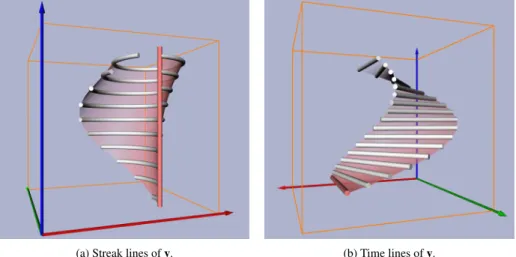
Astreak lineis the connection of all particles set out at different times but the same point location. In an experiment, one can observe these structures by constantly re-leasing dye into the flow from a fixed position. The resulting streak line consists of all particles which have been at this fixed position sometime in the past. Considering the vector fieldpintroduced above, streak lines can be obtained in the following way: apply a stream surface integration inpwhere the seeding curve is a straight line seg-ment parallel to thet-axis, a streak line is the intersection of this stream surface with a hyperplane perpendicular to thet-axis (Figure 2.2a).
Atime lineis the connection of all particles set out at the same time but different
locations, i.e., a line which gets advected by the flow. An analogon in the real world is a yarn or wire thrown into a river, which gets transported and deformed by the flow. However, in contrast to the yarn, a time line can get shorter and longer. It can be obtained by applying a stream surface integration inpstarting at a line witht=const., and intersecting it with a hyperplane perpendicular to thet-axis (Figure 2.2b).
Streak lines and time lines can not be described as tangent curves. Both types of lines fail to have a property of stream and path lines: they are not locally unique, i.e., for a particular location and time there is more than one streak and time line pass-ing through. However, stream, path and streak lines coincide for steady vector fields
v(x,t) =v(x,t0)and are described by (2.9) in this setting. Time lines do not fit into this.
v(x,y,t) = (1−t)· +t·
(a) Tangent curves ofscorrespond to the stream lines inv. See (2.14).
(b) Tangent curves ofpcorrespond to the path lines inv. See (2.13).
Figure 2.1: Characteristic curves of a simple 2D time-dependent vector field shown as illuminated field lines. The red/green coordinate axes denote the(x,y)-domain, the blue axis shows time.
(a) Streak lines ofv. (b) Time lines ofv.
Figure 2.2: Characteristic curves of a simple 2D time-dependent vector field. Seeding curves and resulting stream surfaces are colored red. Same data set as in Figure 2.1.
For two-parameter-dependent vector fieldsv(x,s,t)we consider only stream lines for a given parameter tuple(s,t). Similar to (2.14) they are given as the tangent curves of s(x,s,t) = v(x,s,t) 0 0 . (2.15)
2.1.3
Derived Measures of Vector Fields
A number of measures can be derived from a vector fieldvand its derivatives. These measures indicate certain properties and can be helpful when visualizing flows.
Themagnitudeofvis given as
|v|=pu2+v2+w2. (2.16)
Thedivergenceof a flow field is given as
div(v) =∇·v=trace(J) =ux+vy+wz (2.17) and denotes the gain or loss of mass density at a certain point of the vector field: given a volume element in a flow, a certain amount of mass is entering and exiting it. Diver-gence is the net flux of this at the limit of a point. A flow field with div(v) =0 is called divergence-free, which is a common case in fluid dynamics since a number of fluids
areincompressible.
Thevorticityorcurlof a flow field is given as
ω= ω1 ω2 ω3 =∇×v= wy−vz uz−wx vx−uy . (2.18)
This vector is the axis of locally strongest rotation, i.e., it is perpendicular to the plane in which the locally highest amount of circulation takes place. The vorticity magnitude
|ω|gives the strength of rotation and is often used to identify regions of high vortical activity. A vector field withω=0is calledirrotationalorcurl-free, with the important subclass ofconservativevector fields, i.e., vector fields which are the gradient of a scalar field.
The identification of vortices is a major subject in fluid dynamics. The most widely used quantities for detecting vortices are based on a decomposition of the Jacobian matrixJ=S+Ωinto its symmetric part, the strain tensor
S=1
2(J+J
T) (2.19)
and its antisymmetric part, the vorticity tensor
Ω=1 2(J−J T) = 0 −ω3 ω2 ω3 0 −ω1 −ω2 ω1 0 , (2.20)
withωi being the components of vorticity (2.18). WhileΩassesses vortical activity,
the strain tensorSmeasures the amount of stretching and folding which drives mixing to occur.
Inherent to the decomposition of the flow field gradientJintoSandΩis the
fol-lowing duality: vortical activity is high in regions whereΩdominatesS, whereas strain
is characterized bySdominatingΩ.
In order to identify vortical activity, Jeong et al. used this decomposition in [JH95] to derive the vortex region quantityλ2as the second largest eigenvalue of the symmetric tensorS2+Ω2. Vortex regions are identified byλ2<0, whereasλ2>0 lacks physical interpretation. λ2does not capture stretching and folding of fluid particles and hence does not capture the vorticity-strain duality.
The Q-criterion of Hunt [Hun87], also known as the Okubo-Weiss criterion, is
defined by Q=1 2(kΩk 2− kSk2) =k ωk2−1 2kSk 2. (2.21)
WhereQis positive, the vorticity magnitude dominates the rate of strain. Hence it is natural to define vortex regions as regions whereQ>0. Unlikeλ2,Qhas a physical meaning also whereQ<0. Here the rate of strain dominates the vorticity magnitude.
2.2
Parameter-Independent Topology
In this section we collect the first order topological properties of steady 2D and 3D vector fields.
2.2.1
Critical Points
Considering a steady vector fieldv(x), an isolatedcritical pointx0is given by
v(x0) =0 with v(x0±εεε)6=0. (2.22) This means thatvis zero at the critical point, but non-zero in a certain neighborhood.
Every critical point can be assigned anindex. For a 2D vector field it denotes the number of counterclockwise revolutions of the vectors ofv while traveling counter-clockwise on a closed curve around the critical point.1 Similarly, the index of a 3D critical point measures the number of times the vectors ofvcover the area of an en-closing sphere. The index is always an integer and it may be positive or negative. For a curve/sphere enclosing an arbitrary part of a vector field, the index of the enclosed area/volume is the sum of the indices of the enclosed critical points. Mann et al. show in [MR02] how to compute the index of a region using geometric algebra. A detailed discussion of index theory can be found in [FG82, Got90, Got96].
Critical points are characterized and classified by the behavior of the tangent curves around it. In section 2.4 we give a complete classification of critical points based on sectors of different flow behavior around it. Here, we concentrate on first order critical points, i.e., critical points with det(J(x0))6=0. As shown in [HH89, HH91], a first order Taylor expansion of the flow aroundx0suffices to completely classify it. This is done by an eigenvalue/eigenvector analysis ofJ(x0). Letλibe the eigenvalues of
J(x0)ordered according to their real parts, i.e.,Re(λi−1)≤Re(λi). Furthermore, letei be the corresponding eigenvectors, and letfibe the corresponding eigenvectors of the transposed Jacobian(J(x0))T.2 The sign of the real part of an eigenvalueλi denotes
1For 2D vector fields, it is therefore often called thewinding number.
Figure 2.3: Classification of first order critical points. R1,R2denote the real parts of the eigenvalues of the Jacobian matrix whileI1,I2denote their imaginary parts (from [HH89]).
– together with the corresponding eigenvectorei– the flow direction: positive values represent anoutflowand negative values aninflowbehavior. Based on this we give the classification of 2D and 3D first-order critical points in the following.
2D Vector Fields
Based on the flow direction, first order critical points in 2D vector fields are classified into:
Sources: 0 <Re(λ1)≤Re(λ2) Saddles: Re(λ1)< 0 <Re(λ2) Sinks: Re(λ1)≤Re(λ2)< 0
Thus, sources and sinks consist of complete outflow/inflow, while saddles have a mix-ture of both.
Sources and sinks can be further divided into two stable subclasses by deciding whether or not imaginary parts are present, i.e., whether or notλ1,λ2is a pair of con-jugate complex eigenvalues:
Foci: Im(λ1) =−Im(λ2)6=0 Nodes: Im(λ1) =Im(λ2) =0
There is another important class of critical points in 2D: acenter. Here, we have a pair of conjugate complex eigenvalues withRe(λ1) =Re(λ2) =0. This type is common in incompressible (divergence-free) flows, but unstable in general vector fields since a small perturbation ofvchanges the center to either a sink or a source. Figure 2.3 shows the phase portraits of the different types of first order critical points following [HH89]. The index of a saddle point is−1, while the index of a source, sink, or center is+1. It turns out that this coincides with the sign of det(J(x0)): a negative determinant de-notes a saddle, a positive determinant a source, sink, or center. This already shows that the index of a critical point cannot be used to distinguish or classify them completely, since different types like sources and sinks have assigned the same index.
An iconic representation is an appropriate visualization for critical points, since vector fields usually contain a finite number of them. Throughout this thesis 2D critical points will be displayed as spheres colored according to their classification: sources will be colored in red, sinks in blue, saddles in yellow, and centers in green (Figure 2.4).
(a) Sources (red), sinks (blue) and saddles (yellow) in an example vector field.
(b) Incompressible flow around a cylinder with a saddle (yellow) and a center (green). Data courtesy of Gerd Mutschke (FZ Rossendorf) and Bernd R. Noack (TU Berlin).
Figure 2.4: Critical points of 2D vector fields.
3D Vector Fields
Depending on the sign ofRe(λi)we get the following classification of first-order criti-cal points in 3D vector fields:
Sources: 0 <Re(λ1)≤Re(λ2)≤Re(λ3) Repelling saddles: Re(λ1)< 0 <Re(λ2)≤Re(λ3) Attracting saddles: Re(λ1)≤Re(λ2)< 0 <Re(λ3) Sinks: Re(λ1)≤Re(λ2)≤Re(λ3)< 0
Again, sources and sinks consist of complete outflow/inflow, while saddles have a mix-ture of both. A repelling saddle has one direction of inflow behavior (calledinflow
direction) and a plane in which a 2D outflow behavior occurs (calledoutflow plane).
Similar to this, an attracting saddle consists of anoutflow directionand aninflow plane. Each of the 4 classes above can be further divided into two stable subclasses by deciding whether or not imaginary parts in two of the eigenvalues are present (λ1,λ2,λ3 are not ordered):
Foci: Im(λ1) =0 and Im(λ2) =−Im(λ3)6=0 Nodes: Im(λ1) =Im(λ2) =Im(λ3) =0
As argued in [GTS04b], the index of a first order critical point is given as the sign of the product of the eigenvalues ofJ(x0). This yields an index of+1 for sources and attracting saddles, and an index of−1 for sinks and repelling saddles.
In order to depict 3D critical points, several icons have been proposed in the litera-ture, see [HH91, GLL91, LDG98, HG00, TWHS03, WTHS04a]. Basically, we follow the design approach of [TWHS03, WTHS04a] and color the icons depending on the flow behavior: Attracting parts (inflow) are colored blue, while repelling parts (out-flow) are colored red (Figure 2.5).
(a) Sources and sinks; (a) repelling node and (b) its icon; (c) repelling focus and (d) its icon; (e) attracting node and (f) its icon; (g) attracting focus and (h) its icon.
(b) Repelling and attracting saddles; (a) repelling node saddle and (b) its icon; (c) repelling focus saddle and (d) its icon; (e) attracting node saddle and (f) its icon; (g) attracting focus saddle and (h) its icon.
Figure 2.5: Flow behavior around critical points of 3D vector fields and corresponding iconic representation.
Figure 2.6: Boundary of a 2D vector fieldvconsisting of two inflow parts (red) and one outflow part (blue), which are separated from each other by two boundary switch points. The left one is an outbound point (blue) sincevpoints into the outflow part at this point. The right boundary switch point is an inbound point (red).
2.2.2
Boundary Switch Points and Curves
Letvbe a vector field defined in the domainD⊂IEnandBbe the closed boundary ofD. Under the assumption that the flow is allowed to pass through that boundary, one can distinguish between areas of inflow and outflow onB. These areas are separated from each other byboundary switch points (2D) orboundary switch curves(3D) – being all locations on the boundary where the flow direction is tangential to the boundary. Since these points or curves separate regions of different flow behavior, they are the seeding structures of separatrices emanating from the boundary (see section 2.2.3). In the following we will discuss the properties of boundary switch points/curves for 2D and 3D vector fields separately.
2D Vector Fields: Boundary Switch Points
The boundary of a 2D vector fieldvconsists ofinflow partsandoutflow parts, wherev
points into the domain or out of the domain respectively. These parts are separated from each other by points wherevis tangential to the boundary, i.e.,vpoints neither into the domain nor out of the domain. These points are calledboundary switch points. Two different types exist depending on the behavior of a stream line through it: either the stream line stays inside or outside the domainDin forward and backward integration. Hence, these points are called inbound and outbound points. Following [dLvL99a], an inbound point is characterized byv pointing into the direction of an inflow part. Analogously, at an outbound point,vpoints into the direction of an outflow part. Figure 2.6 gives an illustration.
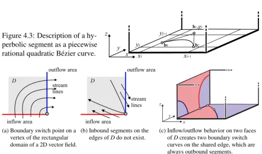
(a) Boundary planez=zminconsisting of an inflow area (red), an outflow area (blue), and their separating boundary switch curve. Shown are 4 vectors ofvon the boundary switch curve, and one each in the inflow and outflow area.
(b) Boundary switch curve consisting of one inbound segment (dark red) and one outbound segment (dark blue). They are separated by an inout point (green).
(c) Inbound pointp0on a boundary switch curve: v(p0)points into the inflow area, ˙v(p0)points
insideD. Shown is a part of the stream line starting inp0both in forward and backward
integration.
(d) Outbound pointp0on a boundary switch curve: v(p0)points into the outflow area, ˙v(p0)points
outsideD. Shown is a stream line close top0
starting in the inflow area and leavingDin the outflow area.
Figure 2.7: Properties of boundary switch curves.
3D Vector Fields: Boundary Switch Curves
In order to ease the explanations in the following, we consider a 3D vector fieldvfrom (2.7) in the domain
D= (xmin,xmax)×(ymin,ymax)×(zmin,zmax) (2.23) withxmin<xmax,ymin<ymax,zmin<zmax. We assume that no critical point ofvlies on the boundary surfaces ofD. Furthermore,Dmight be the whole domain in whichvis defined, or it may be interactively modified and moved around in the data set, leading to a “local topology” [SHJK00].
The boundary surfaces ofD(which are the 6 faces of the bounding box) consist of outflow and inflow areas which are separated byboundary switch curves, i.e., all points on the boundary where the flow direction is tangential to the boundary surface. Figure 2.7a illustrates an example of the boundary plane z=zmin consisting of one inflow and one outflow area. (In the following we illustrate the concept of boundary switch curves only on the boundary planez=zmin. Similar statements hold for the 5 remaining boundary planes ofD.)
In general, boundary switch curves do not intersect each other. The case of inter-secting boundary switch curves can be considered to be structurally unstable: a small perturbation ofvremoves the intersection. Because of this, intersections of boundary switch curves are not considered here.
Given a pointp0on a boundary switch curve, two cases are possible concerning the stream line starting atp0:
• Starting fromp0, the stream line integration moves insideDfor both backward and forward integration. We call this point an inbound pointon the boundary switch curve (Figure 2.7c).
• Starting fromp0, the stream line integration moves outsideDfor both backward and forward integration. Therefore, this stream line in Dconsists only of p0 itself. We call this point anoutbound point(Figure 2.7d).
To distinguish inbound from outbound points, two approaches can be used:
1. Decide whetherv(p0)points into the inflow or the outflow area. Ifv(p0)points into the inflow area, p0is an inbound point. If v(p0) points into the outflow area,p0is an outbound point. This condition corresponds to the classification of boundary switch points for 2D vector fields given in [dLvL99a].
2. Consider the second derivative vector ˙vof the stream lines as a local property ofv(assuming that the tangent vectors of the stream lines are given byv). This gives
˙
v(x,y,z) =∇v·v=uvx +vvy +wvz. (2.24) See [TF97] and [WT02] for details of this. (˙vcan for example be used to compute the curvature of the stream lines in every point ofD: κ=kkv×v˙k
vk3 .) Thenp0is an inbound point if ˙v(p0)points intoD. If ˙v(p0)points out ofD,p0is an outbound point.
Figures 2.7c and 2.7d illustrate both criteria. It can be shown by a straightforward ex-ercise in algebra that both criteria 1 and 2 are equivalent. We preferred to use condition 2, since for a domainDgiven in (2.23), it turns out to be simply a sign check of one component of ˙v.
Inbound points and outbound points form inbound segments andoutbound
seg-mentson the boundary switch curve. These segments are separated byinout points. A
pointp0is an inout point ifv(p0)is parallel to the tangent direction of the boundary switch curve inp0(or equivalently, if ˙v(p0)lies in the tangent plane of the considered boundary ofD). One needs to extract all inout points in order to divide the curve into a number of inbound and outbound segments (Figure 2.7b).
The distinction between inbound segments and outbound segments plays an im-portant role for the topological segmentation of a 3D vector field, because the inbound segments are the seeding curves of the separation surfaces emanating from the bound-ary ofD. Outbound segments do not contribute to separation surfaces in the 3D flow.
2.2.3
Separatrices
Separatrices are stream lines or stream surfaces which separate regions of different flow behavior. Different kinds of separatrices are possible: They can emanate from critical points, boundary switch curves, attachment and detachment lines, or they are closed separatrices without a specific emanating structure.
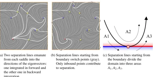
Due to the homogeneous flow behavior around sources and sinks (either a complete outflow or inflow), they do not contribute to separatrices. Each saddle point creates two separatrices: one in forward and one in backward integration into the directions of the eigenvectors. For a 2D saddle point this gives two separation lines (Figure 2.8a). Considering a repelling saddlexRof a 3D vector field, it creates one separation curve (which is a stream line starting inxRin the inflow direction by backward integration) and a separation surface (which is a stream surface starting in the outflow plane by forward integration). Figure 2.9a gives an illustration. A similar statement holds for attracting saddles.
(a) Two separation lines emanate from each saddle into the directions of the eigenvectors: one integrated in forward and the other one in backward integration.
(b) Separation lines starting from boundary switch points (gray). Only inbound points contribute to separation.
(c) Separation lines starting from the boundary divide the domain into three areas A1,A2,A3.
Figure 2.8: Separatrices of a 2D vector field starting from saddles and boundary switch points.
(a) Separatrices of a 3D vector field originating from a repelling node saddle.
(b) Separation surface originating from an inbound segment of a boundary switch curve.
Figure 2.9: Separatrices of a 3D vector field starting from saddles and boundary switch curves.
Considering a stream line starting from a boundary switch point or curve, the stream line integration moves either inside or outside of the domain. Hence, only inbound points or segments play a role for the segmentation of regions of different flow behav-ior inside the domain (see section 2.2.2). Figure 2.8b shows separation lines starting from boundary switch points in a 2D vector field. Figure 2.9b illustrates a separa-tion surface starting from an inbound segment in a 3D vector field. Note that inbound points or segments always create two separatrices: one in forward and one in backward integration. They divide the domain into three areas as shown in Figure 2.8c.
Another type of separatrices, namely closed stream lines, will be discussed in sec-tion 2.2.6.
2.2.4
Saddle Connectors
This section introduces the new concept of saddle connectors, which has been devel-oped in the course of this thesis [TWHS03]. In contrast to 2D vector fields, the set of separatrices of 3D vector fields consists also of stream surfaces (Section 2.2.3) – a fact
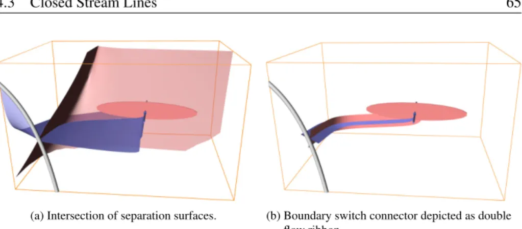
(a) No intersection. (b) Two intersection curves. (c) The separation surfaces collapse.
Figure 2.10: Intersection of separation surfaces.
which creates a number of problems. In particular, we see the following challenges:
• The integration of stream surfaces is computationally more involved and less stable than the integration of stream lines, since convergence and divergence effects on the stream surface may occur.
• The visualization of the topological skeleton of a vector field requires simultane-ous visualization of a higher number of stream surfaces, which very soon leads to visually cluttered representations, since the surfaces hide each other as well as the critical points. This problem remains, even if the separation surfaces are rendered in a semi-transparent mode.
A number of solutions have been proposed for the first problem, see [Hul92, Gel01, SBM+01, vW93].
In this work, we tackle the second problem. In order to create sparse visual rep-resentations that avoid occlusion and minimize visual clutter, we propose to represent the separation surfaces as a finite number of stream lines. These stream lines are the intersection curves of the separation surfaces. We call themsaddle connectorsbecause they start and end in saddle points of the vector field.
The saddle connectors indicate only the approximate run of the separation surfaces and of course cannot completely substitute them. A possible procedure is to always depict the saddle connectors and interactively, on user demand, additionally display
singleseparating surfaces.
The basic idea of saddle connectors is to consider the intersection of the separation surfaces of two saddle points. For this intersection, the following cases are possible:
• The separation surfaces of two saddles have no intersection (Figure 2.10a).
• The separation surfaces have one intersection curve (Figure 2.11a).
• The separation surfaces have more than one, but a finite number of intersection curves (Figure 2.10b).
• The separation surfaces partially collapse. In this case, the intersection of the separation surfaces is a surface (Figure 2.10c).
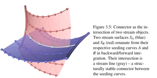
(a) Separation surfaces of the saddles. (b) The intersection of the separation surfaces is the saddle connector.
Figure 2.11: Definition of saddle connectors.
Definition 1 Letvbe a 3D vector field, and letx1andx2be two saddle points inv. We consider the intersection of the two separation surfaces starting in the outflow/inflow planes ofx1andx2. If this intersection is a curve, we call it a saddle connector. Note that this definition excludes cases of partially collapsing separation surfaces. This is justified by the fact that this case can be seen as an unstable situation in the vector field.
An intersection of the separating surfaces of two saddle points can only exist if one of the saddles is an attracting saddle and the other one is a repelling saddle. To see this, imagine for instance two attracting saddles3x
A1,xA2, and suppose that a certain point
plies on both separation surfaces ofxA1andxA2. Then the stream line starting from
pin forward direction must both pass throughxA1andxA2, which contradicts to basic properties of critical points and stream lines.
Also from definition 1 we obtain that a saddle connector is a stream line which starts in the outflow plane of a repelling saddle xR and ends in the inflow plane of an attracting saddlexA. This holds because for every stream surface, the stream line starting from any point on this surface lies completely in the stream surface. Thus, if a pointplies on both separation surfaces ofxRandxA, the whole stream line starting inpin forward and backward direction lies in both separation surfaces. Therefore, this stream line connects both saddles.
One way of analyzing separation surfaces is asking for their boundary curves. If a separation surface does not have a strong diverging behavior, its boundary curve gives a good deal of information about its behavior in the 3D domain ofv. The boundary curve of a separation surface may be a closed curve on the boundary of the domain of
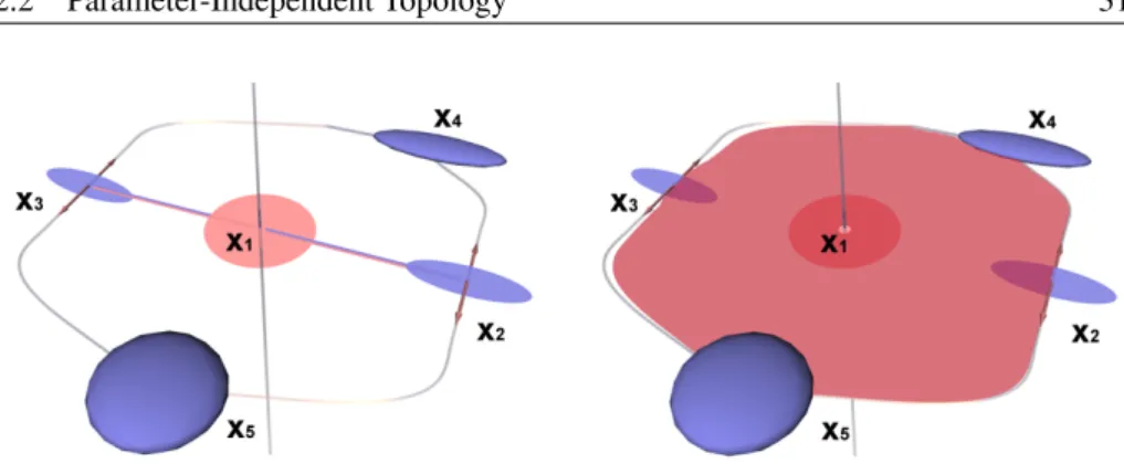
v. It is also possible that the separation surface ends in a number of sinksorsources. In this case, there is a relation between the saddle connectors and the boundary curves of the separation surfaces. To compute the boundary curve of the separation surface of a repelling saddlexR, we can compute the saddle connectors ofxRwith all attracting saddles. Then we consider the repelling separation curves of all attracting saddles which share a saddle connector withxR. If the union of all these curves forms a closed
Figure 2.12: (left) The repelling saddlex1has saddle connectors to the attracting sad-dlesx2andx3. The repelling separation curves ofx2andx3end in the sinksx4andx5, and form a closed curve. (right) The separation curves ofx2andx3are the boundary curves of the separation surface ofx1.
curve, this closed curve describes the boundary curve of the separation surface ofxR. Figure 2.12 shows an example.
2.2.5
Boundary Switch Connectors
As already discussed in section 2.2.3, each inbound segment of a boundary switch curve creates two separation surfaces: one is obtained by applying a forward integra-tion starting from the boundary switch curve, the other one by backward integraintegra-tion. The visualization of these separation surfaces creates the same problems as identified in section 2.2.4 for separation surfaces starting from saddles: if a higher number of separation surfaces is present, their visualization tends to be cluttered due to various occlusion effects.
A solution for this problem is the extension of the idea of saddle connectors: in-stead of visualizing the separation surfaces directly, we compute all intersection curves of these surfaces and visualize this skeleton of curves. In fact, we choose a general approach which yields the intersection curves of all separation surfaces starting either from a saddle point or a boundary switch curve. Analyzing these curves, we obtain the following properties:
• The intersection curves of two separation surfaces are stream lines. This is due to the fact that the intersection of two stream surface is always a stream line (or degenerate).
• Each intersection curve starts either in the outflow plane of a repelling saddle, or on a boundary switch curve by integrating in forward direction.
• Each intersection curve ends either in the inflow plane of an attracting saddle or on a boundary switch curve by integrating in backward direction.
The latter two statements give the following classification regarding the intersection curves of the separation surfaces:
1. The curve starts in a repelling saddle and ends in an attracting saddle. (Figure 2.11)
(a) (b) (c) (d)
Figure 2.13: Boundary switch connectors are the intersection curves of separation sur-faces where at least one surface starts from the boundary.
(a) A closed stream line in a 2D vector field separating two areas of different flow behavior.
(b) The inner closed stream line (blue) acts like a sink, the outer one like a source (red). Figure 2.14: Closed stream lines of 2D vector fields.
2. The curve starts in a repelling saddle and ends in a boundary switch curve. (Fig-ure 2.13a)
3. The curve starts in a boundary switch curve and ends in an attracting saddle. (Figure 2.13b)
4. The curve starts in a boundary switch curve and ends in a different boundary switch curve. (Figure 2.13c)
5. The curve starts in a boundary switch curve and ends in the same boundary switch curve. (Figure 2.13d)
Case 1 refers to saddle connectors as treated in section 2.2.4. Cases 2–5 refer to curves starting or ending in boundary switch curves. Therefore, we call them bound-ary switch connectors. Figure 2.13 illustrates all possible types of boundbound-ary switch connectors.
2.2.6
Closed Stream Lines
Isolated closed stream lines (or periodic orbits) of a 2D vector field are important global topological structures since they separate the vector field into two areas of different
Feature v(x) v(x,t) v(x,s,t)
critical points points curves surfaces
fold / Hopf bifurcations n/a points curves
fold-fold / Hopf-fold bifurcations n/a n/a points
Table 2.1: Dimensionality of topological features for vector fields depending on zero, one or two parameters. Entries marked with “n/a” are either not available in this di-mension or structurally unstable.
flow behavior: inside and outside the closed stream line (Figure 2.14a). Furthermore, they are indicators of recirculating flow behavior. Their influence on the flow is either (Figure 2.14b):
• sink-like, i.e., all stream lines close to the closed stream lineconvergeto it with-out actually reaching it.
• source-like, i.e., all stream lines close to the closed stream linedivergefrom it. Closed stream lines can be found in 3D vector fields as well, but are not treated in this thesis. An analysis of these structures can be found in [Asi93, PS07].
2.3
Parameter-Dependent Topology
The topology of parameter-dependent vector fieldsv(x,a)builds upon the topological properties of steady vector fieldsv(x), i.e., for a fixed set of parametersa=const. the topological structures are identical to the corresponding steady vector fieldv(x)as discussed in section 2.2. However, with a changing set of parametersathe topological structures will change their positions and properties as well. As an example, consider critical points in a vector fieldv(x,t),x∈IRndepending on one parametert(like e.g. a time-dependent flow): critical points move with changingt forming line structures in IRn+1. In a two-parameter-dependent vector field they form surface structures. See Table 2.3 for an overview of the dimensionality of topological features.
Studying the topology of parameter-dependent vector fields means to find the oc-currences of all topological features for the complete parameter spacea∈IEp. In order to understand the dynamics of the data, the following has to be taken into account:
• Correspondence:
One has to find the correspondence between features of different parameter set-tings.
• Bifurcations:
Features might also abruptly change their properties, or they might abruptly ap-pear or disapap-pear at some parameter setting. Such structural changes are called
bifurcationsorevents.
The correspondence problem can be solved in a number of ways. This will be discussed in chapter 5. In the following two sections we will discuss the types of bifurcations that may occur in parameter-dependent vector fields. We focus on structurally stable bifurcations needed to understand the dynamics of flow fields. A detailed introduction to the theory of bifurcations can be found in [GH86].