Edinburgh Research Explorer
Estimating binary spatial autoregressive models for rare events
Citation for published version:
Calabrese, R & Elkink, J 2016, Estimating binary spatial autoregressive models for rare events. in Advances in Econometrics. vol. 37, Advances in Econometrics, vol. 37, Emerald Publishing, pp. 145-166. DOI:
20.500.11820/40014934-d8db-41a0-8d78-59518b52d892, 10.1108/S0731-905320160000037012
Digital Object Identifier (DOI):
20.500.11820/40014934-d8db-41a0-8d78-59518b52d892 10.1108/S0731-905320160000037012
Link:
Link to publication record in Edinburgh Research Explorer
Document Version: Peer reviewed version
Published In:
Advances in Econometrics
Publisher Rights Statement:
'This article is © Emerald Group Publishing and permission has been granted for this version to appear here http://www.research.ed.ac.uk/portal/en/publications/estimating-binary-spatial-autoregressive-models-for-rare-events(40014934-d8db-41a0-8d78-59518b52d892).html Emerald does not grant permission for this article to be further copied/distributed or hosted elsewhere without the express permission from Emerald Group Publishing Limited.'
General rights
Copyright for the publications made accessible via the Edinburgh Research Explorer is retained by the author(s) and / or other copyright owners and it is a condition of accessing these publications that users recognise and abide by the legal requirements associated with these rights.
Take down policy
The University of Edinburgh has made every reasonable effort to ensure that Edinburgh Research Explorer content complies with UK legislation. If you believe that the public display of this file breaches copyright please contact [email protected] providing details, and we will remove access to the work immediately and investigate your claim.
Estimating Binary Spatial Autoregressive Models for
Rare Events
Raffaella Calabrese (University of Essex)
Johan A. Elkink (University College Dublin)
Abstract
The most used spatial regression models for binary dependent variable consider a sym-metric link function, such as the logistic or the probit models. When the dependent variable represents a rare event, a symmetric link function can underestimate the probability that the rare event occurs. Following Calabrese and Osmetti (2013), we suggest the quantile function of the Generalized Extreme Value (GEV) distribution as link function in a spatial generalized linear model and we call this model the Spatial GEV (SGEV) regression model. To estimate the parameters of such model, a modified version of the Gibbs sampling method of Wang and Dey (2010) is proposed. We analyze the performance of our model by Monte Carlo simulations and evaluate the prediction accuracy in empirical data on state failure.
1
Introduction
In this work we analyze rare binary spatial events, i.e. binary dependent variable with spatial dependencies and with a very small number of ones in the sample, usually lower than 5%. In forecasting applications ranging from epidemiology, finance, international relations, to natu-ral disasters, rare events and interdependencies between these events are common. Both the rare event nature of the dependent variable and the spatial autoregressive component generate challenges for the statistical estimation of the model parameters.
When dealing with binary rare events without spatial effects, conventional classification methods, such as logit or probit models, tend to strongly favor the majority class because they are built upon the assumption that every class to be predicted has enough representatives in the data set (Hand et al., 2008). Different authors (e.g., King and Zeng, 2001a,b; Calabrese and Osmetti, 2013; Wang and Dey, 2010) have shown that a symmetric link function leads to very low or even no detection of the minority class when the dependent variable is a rare event.
Some solutions have been proposed to improve the prediction quality of such models for binary rare events without spatial interdependence. King and Zeng (2001a,b) have suggested a correction of the intercept of the logistic regression based on case-control sampling. Ac-cording to Weiss (2004), this proposal has several drawbacks. A different approach has been suggested by Wang and Dey (2010) and Calabrese and Osmetti (2013), based on a flexible skewed link function given by the Generalized Extreme Value (GEV) distribution. This partic-ular distribution is chosen for two main reasons. First, it allows to assign more weight to the information on the minority class. Second, if the minority class is represented by the ones, the
characteristics of the rare events are given by the right tail of the response curve. The variable used in the literature to model the tail of a distribution is the GEV random variable (Kotz and Nadarajah, 2000).
The GEV distribution is characterized by three parameters: a location parameter, a scale pa-rameter and a shape papa-rameter. The main advantage of the GEV distribution is its flexibility—it can be negative and positive skewed. In the first case, more weight is given to the left tail of the response curve and this is more convenient if the minority class is represented by the zeroes. When the GEV link function is positive skewed, the values ones of the dependent variable get more weight, so the minority class should be given by the ones.
Based on our knowledge, this is the first manuscript that analyses the drawbacks caused by a symmetric link function in a spatial regression model for binary rare events. Binary spatial choice models are sufficiently important that LeSage and Pace (2009) focus an entire chapter (Chapter 10) on this topic. In this context, the most used models are probit or logit functional forms with spatial interdependence. Different approaches have been proposed in the literature to estimate these models, e.g. the Gibbs sampling method (LeSage, 2000), the expectation-maximization algorithm (McMillen, 1992), the Generalized Method of Moments (Pinkse and Slade, 1998; Klier and McMillen, 2008) and recursive importance sampling (Beron and Vi-jverberg, 2004). Fleming (2004) and Calabrese and Elkink (2014) compare the properties of these estimators, both theoretically and by Monte Carlo simulations.
To improve the detection of the minority class and following Calabrese and Osmetti (2013), we propose the quantile function of the Generalized Extreme Value (GEV) distribution as link function in a spatial generalized linear model and we call this model the Spatial GEV (SGEV) regression model. To estimate the parameters of such model, a modified version of the Gibbs sampling method of LeSage (2000) and Wang and Dey (2010) is proposed. LeSage (2000) proposes a Gibbs sampler for estimating binary dependent variable models with spatial interdependence, which comparative analysis shows is one of the best estimators available in this context (Calabrese and Elkink, 2014).1 Wang and Dey (2010) propose a Gibbs sampler for rare events using the GEV distribution. We merge the two efforts to develop a new estimator for rare events with spatial autocorrelation.
The SGEV estimator will be evaluated in a series of Monte Carlo simulations, comparing the performance to a number of existing estimators Klier and McMillen (2008); LeSage (2000) for similar data structures, where we evaluate the accuracy of the prediction. In so doing, this research makes a significant contribution to the literatures in spatial econometrics and rare events modeling.
The proposed estimator is of particular relevance to several areas, such as natural science, epidemiology, political science or credit risk. Even if natural disasters (Frei and Schar, 1998; LeSage et al., 2011) or epidemics (Roberts, 2000) occur infrequently, their forecasting is a mandatory activity to reduce the level of risk and damage. In credit risk analysis, there are several contexts where the detection of the minority class is pivotal. Moreover, our proposal could be particularly useful to measure credit contagion, i.e. how the failure of a debtor to fulfill his or her debt obligation can affect the failure propensity of another debtor, on different types of portfolio. For example, if we consider loans to firms, the interdependence is given by the presence of business relations among different firms (Barro and Basso, 2010). As house prices are affected by house locations, credit contagion is important to estimate the failure
1See LeSage et al. (2011) for a corrected, more recent version of this estimator. The estimator proposed below is
propensity of a mortgage loan (Zhu and Pace, 2014). Credit contagion can also be measured on banks as opposed to obligors, such that this approach contributes to the topical literature on systemic risk (Calabrese, Elkink and Giudici, 2014).
Aside from the literature in economics and banking, there are countless application areas in the social sciences more generally. For example, in the political science literature rare events data with spatial or network interdependencies can be found in the study of civil war or in-terstate conflict (e.g. Gleditsch and Ward, 2013), of currency crisis (Novo, 2003), or of state failure (King and Zeng, 2001a,b). The change of political regime from autocracy to democracy is another example where the occurrence of the transition is rare, while they can be expected to be spatially and temporally correlated (Gleditsch and Ward, 2006; Elkink, 2011). The in-terdependence here can be spatial, specified in an exogenously given spatial weights matrix, or based on some alternative network structure such as trade relations or cultural similarity matrices. Following King and Zeng (2001b), who demonstrate the relevance of a rare events estimator by predicting state failure, we provide an empirical application of the SGEV model using updated data on state failure.
Section 2 provides a brief overview of binary regression models with spatially interde-pendent data. Section 3 will outline the estimation complications arising from the nature of rare events data and proposes the use of an asymmetric link function in the binary regression model. Section 4 proposes the Spatial Generalized Extreme Value model for the estimation of rare events data with spatial or network interdependence. Section 5 provides a Monte Carlo analysis to evaluate the statistical performance of the proposed estimator. An initial empirical application is presented in Section 6 and Section 7 concludes.
2
Spatial binary regression models
A widely used representation of a regression model for a binary responseY is the latent re-sponse model (Verbeek, 2008). A continuous variableY∗ is the dependent variable with the observation mechanism
Yi=
1, Y∗>0
0, otherwise. (2.1)
A linear model is specified for this latent response, so the model specification is
Y∗=ρWY∗+Xβββ+εεε, (2.2)
where the error term εεε can follow a multivariate normal distribution in a probit model or a multivariate logistic distribution in a logit model. Wis a spatial lag weights matrix, ρ the
associated scalar parameter,Xa matrix of exogenous variables, andβββthe associated regression
coefficients. W is typically a normalized matrix, whereby all rows add up to one and the diagonal is zero, but see Neumayer and Pl¨umper (2016) for a critique on this convention. For a spatial stationary process,−1<ρ<1.2 This corresponds to the lattice perspective on spatial
data (Anselin, 2002, 255),3which can be directly applied to any other (social) network data—
any application where the dependent variable represents a binary characteristic of the nodes and the edges (i.e.W) are exogenously given.
2WhenWis normalized and maximum likelihood is applied, Anselin (1982) proves that 1/ω
min<ρ<1 to ensure
invertibility of(I−ρW), whereωminis the minimum eigenvalue ofW.
3The altenative, geostatistics, perspective concerns spatial data where space is seen as continuous and observations
From the model (2.2), the Binary Spatial AutoRegressive model (BSAR) is obtained Y∗= (I−ρW)−1(Xβββ+εεε) =A−1Xβββ+e, (2.3)
withA=I−ρWande=A−1εεε(see also McMillen, 1992, 1995; Fleming, 2004).
The variance of the error term follows as
var(e) =varA−1εεε=A−1εεε εεε0[A−1]0. (2.4)
The inherent heteroskedasticity present in matrix (2.4) renders standard binary regression models inconsistent and inefficient (McMillen, 1992), a problem which has been addressed in the literature by the development of various different estimators for BSAR models. We can identify five main estimators of the spatial autocorelation parameterρin this context (see also
Fleming, 2004; LeSage and Pace, 2009).
In the first method, McMillen (1992, 1995) uses an Expectation-Maximization (EM) algo-rithm. The latent variableY∗is replaced with its expected value and the Maximum Likelihood (ML) method is applied. Given the difficulty of estimating both the βββ and εεε εεε0, McMillen
(1992) introduces the assumption of homogeneity for the disturbancesεεε, assuming thatεεε εεε0=
I. Analogously to McMillen (1992), LeSage (2000) also replaces the latent variableY∗ with its expected value, but a Gibbs sampling approach is applied for the parameter estimation. Furthermore, LeSage (2000) removes the assumption of homogeneity, i.e. εεε εεε0=σε2Vwhere
V=diag(v1,v2, . . . ,vn)andviwithi=1,2, . . . ,nare the variance parameters to be estimated.
In the third method, since the likelihood function is a multivariate normal distribution, Beron and Vijverberg (2004) suggest to apply recursive importance sampling (RIS) to the ML esti-mation. Pinkse and Slade (1998) apply a Generalized Method of Moments (GMM) estima-tor. Finally, Klier and McMillen (2008) suggest an approximation of the method proposed by Pinkse and Slade (1998), whereby an extrapolation is applied based on the estimate ofβ when
ρ=0.
Calabrese and Elkink (2014) analyse the properties of the above estimators by Monte Carlo simulations and an empirical application. This study shows that the Gibbs sampler performs best for low values of the spatial autocorrelation parameter and the RIS estimator for high values ofρ. The computationally much more efficient linearized GMM estimator of Klier and
McMillen (2008) performs well under low autocorrelation and large sample size conditions. Because of these properties, we propose a modified version of the Gibbs sampling approach to binary spatial autoregression models, modified for rare events data using an asymmetric link function.
3
Rare events and symmetric link functions
LetY be a Bernoulli random variable with parameterπ=P{Y =1}andxa covariate vector.
The most used regression models for a binary dependent variable are the Generalized Linear Models (GLMs). In GLMs the link functiong(·)is a monotonic function such that
g(π) =β0x,
whereπis the probability of observing the rare event.
For simplicity, the most used link functions are symmetric functions. For example, in the logistic regression model the link functiong(·) is the quantile function of a logistic random
variable g(x) =logit(π(x)) =ln π(x) 1−π(x) =β0x,
which is a symmetric function.
In the probit model, the link function g(·) is the quantile function of a standard normal random variable, which is also symmetric
g(x) =Φ−1(β0x).
When the link function is symmetric, the response curveπ(x)approaches zero at the same
rate it approaches one. This corresponds to the assumption that the same amount of information is included in the observed zeros and ones of the dependent variableY. On the contrary, ifY is a rare event with a low number of ones in the sample, the observed ones are more informative than the observed zeros and should be weighted accordingly in the estimation of the model (Calabrese and Osmetti, 2013; King and Zeng, 2001b). Weighting the zero and one observations equally, when the dependent variableY is a rare event, by using a GLM with a symmetric link function, potentially underestimates the probabilityπ for the observed ones (Calabrese and Osmetti, 2015; King and Zeng, 2001b).
Furthermore, when the probability of an event is low and the sample size reasonably large, the binomial distribution can be, and commonly is, approximated by a Poisson distribution (Falk, H¨usler and Reiss, 2010, 4–5), which is a skewed distribution. It is therefore more consistent to also choose an asymmetric link function for binary regression models dealing with such rare events.
In order to overcome these drawbacks, different methods have been proposed in the liter-ature. The most widely used approach is choice-based or case-control sampling with a cor-rection on the parameter estimates (David H. Good and Sickles, 1986; King and Zeng, 2001a; Manski and Lerman, 1977; McCullagh and Nelder, 1989; Scott and Wild, 1986). In the sur-vival analysis context, the cure model (Lambert and Thompson, 2007) and the mixture hazard model (Almanidis and Sicles, 2015) are also used. Instead, Wang and Dey (2010) and Cal-abrese and Osmetti (2013) propose to focus the attention on the right tail of the response curve that represents the feautures of ones.
Since the GEV distribution function is used in the literature (e.g. Kotz and Nadarajah, 2000; Falk, H¨usler and Reiss, 2010) to represent the tail of a random variable, Wang and Dey (2010) and Calabrese and Osmetti (2013) propose the quantile function of a GEV random variable as a link function in a GLM. The main difference between these two proposals is that Wang and Dey (2010) use a Bayesian approach to estimateβ and the shape parameter of the GEV
distribution and Calabrese and Osmetti (2013) estimateβ by the ML method, while they keep
the shape parameter fixed. Instead of estimating the shape parameter, Calabrese and Osmetti (2013) propose to fit as many models as the number of chosen values of the shape parameter and select the model that yields the highest predictive accuracy.
4
The Spatial Generalized Extreme Value (SGEV)
re-gression model
The aim of this section is to propose a new spatial regression model for binary responses with unequal sample frequencies of the two outcomes that overcome the drawbacks outlined in
Section 3. Following Wang and Dey (2010) and Calabrese and Osmetti (2013), we consider a quantile function of a GEV distribution as the link function in a binary regression model and extend this to model spatial interdependence. Hence, we propose the Spatial Generalized Extreme Value (SGEV) regression model
π(x) =exp n − 1+τD−1A−1Xβββ−+1/τ o , (4.5)
wherex+=max(x,0)andD=diag(σσσe)is the diagonal matrix, with elementsσσσethat repre-sent the root square of the diagonal elements in matrix (2.4).
Since a GEV response curve can be asymmetric, the underestimation ofP{Y =1}for the observation equal to one may be overcome. Another advantage of the GEV distribution is that it is very flexible with the tail shape parameter τ controlling the shape and size of the
tails, with three different families of distributions subsumed under it. The Type II (Fr´echet-type distribution) and the Type III (Weibull-(Fr´echet-type distribution) classes of the extreme value distribution correspond respectively to the case whereτ>0 andτ<0, while the Type I class
(Gumbel-type distribution) arises in the limit asτ→0, Fr´echet and Weibull distributions are
related by a change of sign. Forτ→0 andρ =0, the SGEV regression model becomes the
response curve of the log-log model (e.g. Agresti, 2002).
The main estimators proposed in the literature for spatial regression models are analysed in Section 2. Since the Gibbs sampling approach (LeSage, 2000) provides accurate estimates of the parameter ρ under a wide range of different Monte Carlo parameters (Calabrese and
Elkink, 2014), we propose a modified version of this method to estimate the SGEV model (4.5). We make use of the Gibbs sampler for the non-spatial GEV model proposed by Wang and Dey (2010). While LeSage (2000) makes use of the Metropolis-Hastings algorithm for the estimation of the spatial parameterρ, Wang and Dey (2010) use this algorithm for all model
parameters. We follow Wang and Dey (2010)’s approach, which provides more accurate and computationally more efficient results.4
The joint posterior distribution of the parameter vectorθθθ= [βββ0,τ,ρ]0is given by
φ(θθθ/y,X)∝L(y/X,θθθ)ν(θθθ)
where the likelihood
L(y/X,θθθ) = N
∏
i=1 πi(θθθ)yi[1−πi(θθθ)]1−yi (4.6)andπ(·)is defined in equation (4.5).5 To assign the priors of the SGEV model, we use LeSage
(2000)’s assumption that the priors are independent
ν(θθθ) =ν(ρ,βββ,ρ) =ν(ρ)ν(βββ)ν(V),
where we follow Wang and Dey (2010) in assigning a relatively uninformative prior distri-bution ofN(0,100)to all parameters. Using the estimates of a non-spatial log-log model as the initial values βββ0, the correlation between y andWy as the initial value ρ0, and τ0 =0, 4This will also allow further improvements, since there is a flourishing literature on optimizing Metropolis-Hastings
algorithms (e.g. Maclaurin and Adams, 2014; Korattikara, Chen and Welling, 2014; Angelino et al., 2014).
5We assumeεεε εεε0=
σε2I. The parameterσε2is kept fixed, because of lack of identifiability when simultaneously estimating the error variance and the linear regression coefficients in a latent variable model—similar to probit and logit regressions.
all estimates are updated in each Markov Chain Monte Carlo (MCMC) iteration through the Metropolis-Hastings algorithm.
The Metropolis-Hastings algorithm (Hastings, 1970) proceeds as follows. For eachθj, let
the valueθ∗j,t+1=θj,t+cZ be generated, whereZ is a draw from a standard normal
distribu-tion,cis a known constant, andt refers to the sampling iteration. Defining the log-likelihood l(y/X,θθθ) =log[L(y/X,θθθ)], the acceptance probability
a=min 1,l(y/X,θθθ ∗ t+1)ν(θθθ) l(y/X,θθθt+1)ν(θθθ) ,
whereθθθ∗t+1=θθθt+1, except for parameterθ∗j,t+1. A valuemis drawn from a continuous uniform
distribution with support[0,1]. Ifm<a, the next draw from the density function (4.6) is given by θj,t+1=θ∗j,t+1, otherwise the draw is taken to be the current valueθj,t+1 =θj,t. Where
the parameter is constrained,Zis drawn from a truncated standard normal distribution—in our application this holds for ρ, which is constrained to the [−1,1]interval. For computational
efficiency reasons and following Thomas (2007), we dynamically adaptcthroughout the chain for each parameter inθθθ, such that the acceptance rate of the Metropolis-Hastings algorithm is
approximately 20%.6
5
Monte Carlo simulations
In order to evaluate the performance of the proposed estimator, we perform Monte Carlo anal-yses whereby the estimator is applied to data of which the underlying data generation mecha-nism, and its associated parameters, are known. While the Monte Carlo analysis in Calabrese and Elkink (2014) focuses primarily on the estimation of the intensity of the spatial autocorre-lation,ρ, we focus primarily on the prediction quality of the estimator.
The data generation process results in four continuous independent variables, with for each X ∼N(0,4σε), withσε =1. The residuals vectorεεε is generated from a multivariate normal distributionNn(0,I).
We performed the simulations usingN=500 as sample size and a parameter vectorβββ =
[0,1,1,−1,−1]0. The level of spatial autocorrelation is varied from entirely absent to high autocorrelation,ρ∈ {0,0.1,0.45,0.8}. Finally, as we handle two-class classification problems
with highly unbalanced class sizes, the dependent variable Y is constructed by applying a threshold different from the zero in (2.1), such that the proportion of ones is predetermined, in these simulations to 20% and 5%. We thus end up with eight different configurations of the data generation parameters. We perform estimations on 60 replications of each parameter configuration.
In order to generate the matrixW, we apply the method suggested by Beron and Vijverberg (2004, 179). We assign each observation randomly to a coordinate in the unit square using a uniform distribution. For each observation, those observations that are within a fixed radius, excluding the observation itself, are considered neighbours. The radiusd is set such that the average number of neighbours for each observation is approximately 5, identical to Beron and Vijverberg (2004), which impliesd=0.06 forN=500.
The main aim of the SGEV model is to improve the accuracy of predicting the rare events, the ones. Hence, the applications of our proposal are classification problems where perform-ing an incorrect prediction of the rare event may have grave consequences. For example, in
mushroom classification judging a poisonous mushroom to be edible is far worse than judging an edible mushroom to be poisonous. In the context of our empirical example, the prediction of state failure, it is also reasonable to assume that it is more important not to miss a poten-tial future failed state than that it is to slightly overestimate the probability of state failure for a state that is less at risk. A similar rationale applies to the risk of bank defaults, currency defaults or default on credits, where (central) banks will be more concerned with correctly identifying those cases that are truly at risk than with incorrectly identifying some cases as at risk while they are not. Applying a similar logic to credit defaults, Calabrese and Osmetti (2013) therefore calculate the Mean Absolute Error (MAE+) and Mean Squared Error (MSE+) for the subset of cases whereY =1
MAE+= 1 N{y
∑
i=1} [yi−πˆi] MSE+= 1 N{y∑
i=1} [yi−πˆi]2. (5.7)We compare the SGEV model with the predictive performance of the estimators proposed by Klier and McMillen (2008) (denoted as KM) and LeSage (2000) (denoted as GibbsT). Within a certain range of values of the shape parameterτ, the usual regularity conditions for
the estimator of this parameter do not hold (Smith, 1985). For this reason, we report the results of the SGEV model with the estimation ofτ (denoted as SGEV), as explained in the previous
Section, and fixing the parameterτ to 25 (denoted as SGEVfix).7 Finally, three GLMs with
asymmetric link functions that ignore the spatial interdependence are considered: the cloglog model, the GEV model proposed by Calabrese and Osmetti (2015)8(denoted as BGEVA) and the GEV model proposed by Wang and Dey (2010) (denoted as GEV WD).9
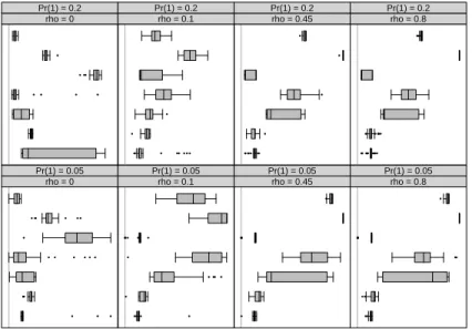
The plot in Figure 1 provides a graphical depiction of the MSE+defined in equation (5.7). This plot shows that for 20% of ones, the SGEV model outperforms the other models when the spatial autocorrelationρ increases. When the sample is strongly unbalanced (i.e. 5% of ones)
and in the presence of spatial interdependence, the accuracy of identifying the ones in the data set is notably better for the SGEV estimator. This is of course not surprising, given that the proposed model is designed to address the prediction of rare events in the presence of spatial interdependence.
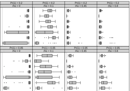
While we emphasise the importance of correctly predicting high probabilities for the rare outcome ofY =1, the estimator still needs to classify the cases for both positive and negative outcomes. In other words, while we can prioritize a low true positive rate over a low false positive rate, we still need to make sure that our classifier identifies both negative and positive cases. The plot in Figure 2 therefore provides the overall Mean Squared Error, including both yi=1 andyi=0 cases. It is clear from this plot that, while positive cases are generally better
identified by the SGEV estimator, this is combined with a relatively high false positive rate. Since the prediction of ones and zeros can be sensitive to the choice of the prediction threshold—the predicted probabilityP(Y=1)above which we predict a 1—alternative statis-tics are available that consider the entire range of potential threshold values. A common pro-cedure is to sort all predicted values ˆy∗, then move the decision threshold along the range of values, and plot the proportion of correctly classified ones against the proportion of incorrectly classified ones. This is referred to as the Receiver Operating Charateristic (ROC) curve (see, e.g., Hand and Anagnostopoulos, 2014) and is often used to compare the classification quality
7We considered different values of the parameterτ and we chose the one that shows the best predictive
perfor-mance.
8The R package BGEVA (Marra, Calabrese and Osmetti, 2013) is used to estimate the GEV model.
Mean Squared Error for Y=1 Estimator SGEV SGEVfix GibbsT KM SGEV_WD BGEVA cloglog 0.0 0.2 0.4 0.6 0.8 1.0 ● ● ● ●●● ● ● ● ●●● ● ● ● ● ● ●● ● rho = 0 Pr(1) = 0.05 0.0 0.2 0.4 0.6 0.8 1.0 ● ● ● ● ● ● ●● ● ● ●● ● ●● ● rho = 0.1 Pr(1) = 0.05 0.0 0.2 0.4 0.6 0.8 1.0 ● ●●●●●● ● rho = 0.45 Pr(1) = 0.05 0.0 0.2 0.4 0.6 0.8 1.0 ● ● ● ● ●● ● ●●●●●●● ● rho = 0.8 Pr(1) = 0.05 SGEV SGEVfix GibbsT KM SGEV_WD BGEVA cloglog ●● ● ● ● ●● ● rho = 0 Pr(1) = 0.2 ● ●● ● ● ● ● ● ● ● rho = 0.1 Pr(1) = 0.2 ●●●● ●● ● ● ● ● ● rho = 0.45 Pr(1) = 0.2 ● ● ●● ● ● ● ●● ●● ● ● ● ●●●●● ● ●●●● rho = 0.8 Pr(1) = 0.2
Figure 1: Distribution of the MSE+ for y=1 defined in equation (5.7) for different configurations of the parameters, across 60 replications.
Mean Squared Error
Estimator SGEV SGEVfix GibbsT KM SGEV_WD BGEVA cloglog 0.0 0.2 0.4 0.6 0.8 1.0 ● ● ● ●●● ●● ●● ● ● ● ●● ●● ●● ● ●● ●●● ● rho = 0 Pr(1) = 0.05 0.0 0.2 0.4 0.6 0.8 1.0 ● ● ● ● ● ●● ● rho = 0.1 Pr(1) = 0.05 0.0 0.2 0.4 0.6 0.8 1.0 ● ●●●● ● ● ● rho = 0.45 Pr(1) = 0.05 0.0 0.2 0.4 0.6 0.8 1.0 ● rho = 0.8 Pr(1) = 0.05 SGEV SGEVfix GibbsT KM SGEV_WD BGEVA cloglog ● ● ● ● ● ● ● ● rho = 0 Pr(1) = 0.2 ● ● ● ● ●● ● rho = 0.1 Pr(1) = 0.2 ●●● ● ● rho = 0.45 Pr(1) = 0.2 ●●● rho = 0.8 Pr(1) = 0.2
Figure 2: Distribution of the Mean Squared Error for different configurations of the parameters, across 60 replications.
H−index Estimator SGEV SGEVfix GibbsT KM SGEV_WD BGEVA cloglog 0.0 0.2 0.4 0.6 0.8 1.0 ● ●● ● ● ●●● ●● ● ● ● ●●● ● ● ● ● ● rho = 0 Pr(1) = 0.05 0.0 0.2 0.4 0.6 0.8 1.0 ● ● ● rho = 0.1 Pr(1) = 0.05 0.0 0.2 0.4 0.6 0.8 1.0 ●●● ● ● ● ● rho = 0.45 Pr(1) = 0.05 0.0 0.2 0.4 0.6 0.8 1.0 ● ● ● ●● rho = 0.8 Pr(1) = 0.05 SGEV SGEVfix GibbsT KM SGEV_WD BGEVA cloglog ● ● ● rho = 0 Pr(1) = 0.2 ● ● ●● ● ●● ● ● ● rho = 0.1 Pr(1) = 0.2 ● ● ● ●● ● ● ● ● ● rho = 0.45 Pr(1) = 0.2 ● ● ● ● ● ● ● ● ● ● ●● ●● ● ● ● ● rho = 0.8 Pr(1) = 0.2
Figure 3: Distribution of the H-index, for different configurations of the parameters, across 60 replications.
of different models or algorithms. The curve will generally be above the 45 degree diagonal line, since otherwise we could simply create a better classifier by swapping the labelling of the predictions. The further the ROC curve from the diagonal line, the better the classifier. A numerical indicator for this prediction quality is the Area Under Curve (AUC) statistic, which is the area under the ROC curve, and thus ranges typically from 0.5 to 1—an AUC below 0.5 indicates a classifier performing worse than random classification of cases.
The AUC statistic suffers from a number of deficiencies as a measure to evaluate the performance of different estimators. A particular feature of the statistic that is of concern to our Monte Carlo study is the fact that this statistic amounts to a weighted average min-imum loss measure. This average loss is determined by the relative cost of misclassifying zeros or ones, whereby the cases are weighted depending on the cumulative density func-tion of the two classes across the range of scores (that is, F0(t) =Pr[yˆ∗(x)<t|Y=0]and
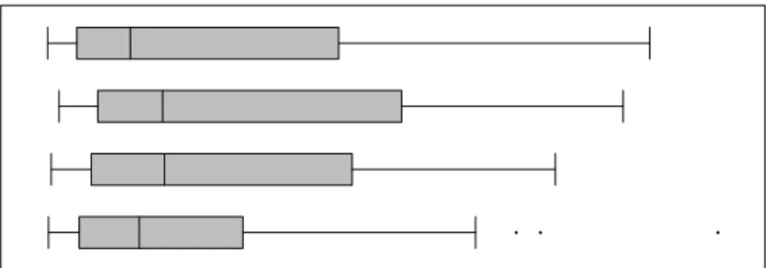
F1(t) =Pr[yˆ∗(x)<t|Y =1], with score ˆy∗(x)the prediction of the classifier andtthe thresh-old value) (Hand, 2009, 108–111). In other words, the relative cost of misclassifying ones or zeros—and thus the evaluation of the relative performance of the classifier—are dependent on the classifier used, as opposed to being dependent on the underlying application, which is incoherent. Hand (2009) and Hand and Anagnostopoulos (2013, 2014) outline this complica-tion and provide an alternative to the AUC score, the so-calledH-index, which addresses this deficiency. TheH-index has a range of 0 to 1, with high values indicating improved perfor-mance. We use thehmeasurepackage in R (Anagnostopoulos and Hand, 2012) to calculate theH-index statistics, the results of which are summarized in Figure 3.
Coherently with the results shown in Figure 1, we again see a relatively better performance for the SGEV model compared to the others in Figure 3, when the sample is strongly imbal-anced and the spatial autocorrelation parameterρ increases.
6
Empirical application to state failure
We investigate the performance on empirical data by using an application from comparative politics, on state failure. State failure refers to a state losing the capacity to control its territory and implement domestic policies, due to for example civil war. The prediction of state failure is also the core example of the earlier work on models for rare events by King and Zeng (2001a). State failures can be expected to be “contagious” for a number of reasons (Iqbal and Starr, 2008). Indeed, there is extensive research on the spatial diffusion of civil war (see, e.g., Buhaug and Gleditsch, 2008; Starr, Darmofal and Iqbal, 2008). Instability in one country and lack of capacity by the state can create a safe haven for potential rebels in a neighboring country. Civil conflict is often related to ethnic divisions, which tend to cross national boundaries. Reduced state capacity due to extreme natural events, such as droughts, will also typically affect adjacent countries. Finally, rebellion and civil war in a neighboring country can act as an example for groups within a country. Such effects are clearly visible in, for example, the Arab Spring in 2011, when rebellious behavior in one state soon affected similar acts in a wide region. The spatial clustering of instability and civil war is well established, but the debate on the causal explanations of this clustering ongoing.
To test the model on data related to state failure, we use a definition of W that is based on the inverse distance between two states, whereby the distance is defined as the shortest distance between the two state borders. Since the inverse of the distance is undefined when the distance is zero, and because the inverse has a very fast decay, with slightly larger distances having minimal effect, we use a slowly decaying function by distance,wi jt=1/(di jt+100),
withwiit=0 anddi jtthe minimum geographical distance between countriesiand jat timet.10
ThisWmatrix is a block-diagonal matrix, with the inverse distances on the blocks along the diagonal and zeros otherwise – i.e. one block for each time periodt. ThisWis subsequently normalized such that all rows add up to one.
The model specification we use is inspired by, but does not closely follow, Goldstone et al. (2010). In their replication data, specific matched samples are used to address the rare events nature of the data, while we estimate our models on a full data set of all countries and years where we have data on the relevant variables. All independent variables are lagged by one year relative to the dependent variable. To account for world-wide shocks, year dummies are included. The independent variables are sourced from the Nations, Development, and
Democracydata set by Wejnert (2007) and the data used is from 1975 onwards.
Table 1 provides the regression estimates for the four models on identical data,11 with in addition the H-index measure of prediction quality. Strikingly, while for the Monte Carlo analysis the SGEV estimator performed well in the presence of spatial autocorrelation, in this empirical data the results appear weaker—for the within-sample prediction of the outcome variable, the H-index suggests a marginally better classifier than logistic regression without accommodation of spatial or skewed effects.
The estimate for the autoregression parameterρ by the regular Gibbs sampler, which it is
generally good at estimating (Calabrese and Elkink, 2014), suggests an absence of, or even negative spatial autocorrelation—the 95% Highest Posterior Density interval is[−0.37,0.22], with 82% of the posterior samples providing an estimate ofρbelow zero. The same negative
coefficient is identified by the SGEV estimator whenτ is fixed. The weak predictive results of
the SGEV estimator might therefore be due to lack of actual spatial autocorrelation in this data,
10The minimum distance is calculated using thecshapespackage in R (Weidmann and Gleditsch, 2010). 11For computational efficiency reasons, the data is a subset of the overall data set.
Logistic Gibbs BGEVA SGEVfix SGEV intercept -17.08 -3.50 -3.69 -6.43 -134.78 Polity IV -0.03 -0.01 -0.04 -6.48 -0.34 Polity IV squared -0.01 -0.02 -0.02 5.43 5.25 Log of infant mortality 0.17 0.44 0.51 -41.97 -4.09 Log of GDP per capita -0.51 0.06 -0.02 3.76 -4.88
ρ -0.17 -0.10 0.28
τ 25.00 25.00 126.92
N 1653 324 324 324 324
H-index 0.467 0.432 0.433 0.471 0.471
Table 1: Regressions explaining state failure as classified in Goldstone et al. (2010), using a slowly decaying inverse of the distance to define the adjacency matrix. Models include year fixed effects and the dependent variable is observed at t+1. For the BGEVA and SGEVfix models,τ is fixeda priori.
at least when the spatial contiguity matrix is defined as a matrix of inverse distances between countries.
While the paper is primarily concerned with the accurate prediction of the rare event, the empirical results do raise the question whether the estimation ofτ in particular is problematic.
Figure 4 provides some insight into the performance of the SGEV estimator when it comes to correctly identifying the shape parameter τ. Strikingly, under the absence of any spatial autocorrelation, the estimates ofτ are reasonably accurate, albeit with high variance. Under
spatial autocorrelation, however (ρ=0.5), the estimates ofτ are nearly always zero, which is
the initial valueτ0.
7
Conclusion
In this paper we propose a spatial regression model for highly imbalanced binary data, i.e. data whereby the classification categories are not approximately equally represented. Specifically, the category less represented is considered a rare event with its percentage in the sample lower than 5%. In this context, a symmetric link function, such as the logit or the probit function can underestimate the probability that the rare event occurs. To overcome this drawback, a generalized linear model with a flexible link function given by the GEV distribution is proposed in the literature (Calabrese and Osmetti, 2013; Wang and Dey, 2010).
Many applications where such rare events occur also contain spatial or network interde-pendencies. Examples include systemic risk for banks, eruption of international conflict, or currency crises. We therefore propose a generalized linear model based on the GEV distribu-tion, taking into account spatial or network interdependence, the SGEV model. We provide a modified version of the Gibbs sampling method LeSage (2000); Wang and Dey (2010) to estimate the parameters of the proposed model. The shape parameter of the GEV distribution regulates the skewness. In this paper, we both estimate the shape parameter and fix it in order to obtain lower errors.
Tau Rho rho = 0 rho = 0.1 rho = 0.45 rho = 0.8 50 100 150 200 250 ● ● ●
Figure 4: Distribution of the estimates ofτ, for different configurations of the
param-eters, across 60 replications.
compare the predictive accuracy of our proposal with that of the spatial Gibbs sampler LeSage (2000) and the linearized Generalized Method of Moments Klier and McMillen (2008). The current implementation provides a high true positive rate—the rare events are generally cor-rectly identified—but also a relatively high false positive rate. TheH-index however, which is used for the evaluation of the overall prediction quality for imbalanced samples, shows a slightly better performance of our estimator than existing estimators, in the presence of spatial autocorrelation.
A brief example from the political science literature is used to demonstrate the applicability of the model, namely by investigating the rare occurance of state failure. This is based on the data used in published work on rare events. The SGEV estimator outperforms the other estimators as measured by theH-index. Future work will include applications to systemic risk for banks and credit risk. Furthermore, future research should be able to improve the estimation of the shape parameterτ. One direction of research in this regard might be the use of Bayesian
model selection. Finally, while this paper, in line with Calabrese and Elkink (2014), focuses on the spatial autoregressive model, a similar extension can also be developed for the spatial error model, whereby the network interdependence is modeled in the error term as opposed through the spatially lagged dependent variable.
References
Agresti, Alan. 2002. Categorical data analysis. 2nd ed. New York: Wiley.
Almanidis, Pavlos and Robin C. Sicles. 2015. “Banking Crises, Early Warning Models, and Efficiency.” Working paper.
Anagnostopoulos, Christoforos and David J. Hand. 2012.hmeasure: The H-measure and other scalar classification performance metrics. R package version 1.0.
Angelino, Elaine, Eddie Kohler, Amos Waterland, Margo Seltzer and Ryan P. Adams. 2014. “Accelerating MCMC via parallel predictive prefetching.” arXiv preprint arXiv:1403.7265. Anselin, Luc. 1982. “A note on small sample properties of estimators in a first-order spatial
autoregressive model.”Environment and Planning14(1):1023–1030.
Anselin, Luc. 2002. “Under the hood. Issues in the specification and interpretation of spatial regression models.”Agricultural Economics27:247–267.
Barro, Diana and Antonella Basso. 2010. “Credit contagion in a network of firms with spatial interaction.”European Journal of Operational Research205:459–468.
Beron, Kurt J. and Wim P.M. Vijverberg. 2004. Probit in a spatial context: a Monte Carlo analysis. In Advances in spatial econometrics. Methodology, tools and applications, ed. Luc Anselin, Raymond J.G.M. Florax and Sergio J. Rey. Berlin: Springer pp. 169–195. Bivand, Roger. 1998. “A review of spatial statistical techniques for location studies.” Paper
presented at the CEPR symposium on New Issues in Trade and Location (2277), Lund, Sweden, 28-30 August, 1998.
Buhaug, Halvard and Kristian S. Gleditsch. 2008. “Contagion or clustering? Why conflicts cluster in space.”.
Calabrese, Raffaella and Johan A. Elkink. 2014. “Estimators of binary spatial autoregressive models: A Monte Carlo study.”Journal of Regional Science54(4):664–687.
Calabrese, Raffaella, Jos Elkink and Paolo Giudici. 2014. Measuring Bank Contagion in Eu-rope Using Binary Spatial Regression Models. Technical report. Department of Economics and Management, University of Pavia.
Calabrese, Raffaella and Silvia A. Osmetti. 2013. “Modelling small and medium enterprise loan defaults as rare events: The generalized extreme value regression model.” Journal of Applied Statistics40:1172–1188.
Calabrese, Raffaella and Silvia Osmetti. 2015. “Improving Forecast of Binary Rare Events Data: A GAM-Based Approach.”Journal of Forecasting34(3):230–239.
David H. Good, Maureen A. Pirog-Good and Robin C. Sickles. 1986. “An Analysis of Youth Crime and Employment Patterns.”Journal of Quantitative Criminology2(3):219–236. Elkink, Johan A. 2011. “The international diffusion of democracy.” Comparative Political
Studies44(12):1651–1674.
Falk, Michael, J¨urg H¨usler and Rolf-Dieter Reiss. 2010. Laws of Small Numbers: Extremes and Rare Events. Springer.
Fleming, Mark M. 2004. Techniques for estimating spatially dependent discrete choice models. InAdvances in spatial econometrics. Methodology, tools and applications, ed. Luc Anselin, Raymond J.G.M. Florax and Sergio J. Rey. Berlin: Springer pp. 145–167.
Frei, Christoph and Christoph Schar. 1998. “A precipitation climatology of the Alps from high-resolution reain-gauge observations.”International Journal of Climatology18:873–900. Gleditsch, Kristian S. and Michael D. Ward. 2006. “Diffusion and the international context of
democratization.”International Organization60(4):911–933.
Gleditsch, Kristian S. and Michael D. Ward. 2013. “Forecasting is difficult, especially about the future: Using contentious issues to forecast interstate disputes.”Journal of Peace Re-search50(1):17–31.
Goldstone, Jack A., Robert H. Bates, David L. Epstein, Ted Robert Gurr, Michael B. Lustik, Monty G. Marshall, Jay Ulfelder and Mark Woodward. 2010. “A global model for forecast-ing political instability.”American Journal of Political Science51(1).
Hand, David J. 2009. “Measuring classifier performance: A coherent alternative to the area under the ROC curve.”Machine Learning77:103–123.
Hand, David J., Chris Whitrow, Niall M. Adams, Piotr Juszczak and Dave Weston. 2008. “Per-formance criteria for plastic card fraud detection tools.” Journal of Operational Research
Society59(7):956–962.
Hand, David J. and Christoforos Anagnostopoulos. 2013. “When is the area under the receiver operating characteristic curve an appropriat emeasure of classifier performance?” Pattern
Recognition Letters13:492–495.
Hand, David J. and Christoforos Anagnostopoulos. 2014. “A better Beta for theHmeasure of classification performance.”Pattern Recognition Letters40:41–46.
Hastings, W. Keith. 1970. “Monte Carlo sampling methods using Markov chains and their applications.”Biometrika57:97–109.
Iqbal, Zaryab and Harvey Starr. 2008. “Bad neighbors: Failed states and their consequences.”
Conflict Management and Peace Science25:315–331.
King, Gary and Langche Zeng. 2001a. “Explaining Rare Events in International Relations.”
International Organization55:693–715.
King, Gary and Langche Zeng. 2001b. “Logistic Regression in Rare Events Data.”Political
Analysis9:137–163.
Klier, Thomas and Daniel P. McMillen. 2008. “Clustering of auto supplier plants in the United States: generalized method of moments spatial logit for large samples.”Journal of Business & Economic Statistics26(4):460–471.
Korattikara, Anoop, Yutian Chen and Max Welling. 2014. “Austerity in MCMC land: Cutting the Metropolis-Hastings budget.” arXiv preprint arXiv:1304.5299.
Kotz, Samuel and Saralees Nadarajah. 2000. Extreme Value Distributions. Theory and Appli-cations. Imperial College Press, London.
Lambert, Paul C. and John R. Thompson. 2007. “Estimating and modeling the cure fraction in population-based cancer survival analysis.”Biostatistics8(3):576–594.
LeSage, James P. 2000. “Bayesian estimation of limited dependent variable spatial autoregres-sive models.”Geographical Analysis32(1):19–35.
LeSage, James P., R. Kelley Pace, Nina Lam, Richard Campanella and Xingjian Liu. 2011. “New Orleans business recovery in the aftermath of Hurricane Katrina.”Journal of the Royal Statistical Society: Series A (Statistics in Society)174(4):1007–1027.
LeSage, James P. and Robert Kelley Pace. 2009. Introduction to Spatial Econometrics. CRC Press.
Maclaurin, Dougal and Ryan P. Adams. 2014. “Firefly Monte Carlo: Exact MCMC with subsets of data.” arXiv preprint arXiv:1403.5693.
Manski, C. F. and S. R. Lerman. 1977. “The Estimation of Choice Probabilities from Choice-based Samples.”Econometrica45(8).
Marra, Giampiero, Raffaella Calabrese and Silvia Angela Osmetti. 2013. “Package ‘bgeva: Generalized Extreme Value Additive Modelling for binary rare events data’.”.
URL:https://cran.r-project.org/web/packages/bgeva.pdf
McCullagh, Peter and John A. Nelder. 1989. Generalized linear models. 2nd ed. New York: Chapman and Hall.
McMillen, Daniel P. 1992. “Probit with spatial autocorrelation.”Journal of Regional Science 32(3):335–348.
McMillen, Daniel P. 1995. Spatial effects in probit models: a Monte Carlo investigation.
In New directions in spatial econometrics, ed. Luc Anselin and Raymond J.G.M. Florax.
Berlin: Springer Verlag pp. 189–228.
Neumayer, Eric and Thomas Pl¨umper. 2016. “W.”Political Science Research and Methods 4(1):175–193.
Novo, lvaro A. 2003. Contagious currency crisis: A spatial probit approach. Working papers Banco de Portugal, Economics and Research Department.
URL:http://EconPapers.repec.org/RePEc:ptu:wpaper:w200305
Pinkse, Joris and Margaret E. Slade. 1998. “Contracting in space: an application of spatial statistics to discrete-choice models.”Journal of Econometrics85:125–154.
Roberts, Stephen J. 2000. “Extreme value statistics for novelty detection in biomedical data processing.”Science, Measurement and Technology, IEE Proceedings147:363–367. Scott, Alastair and Chris Wild. 1986. “Fitting Logistic Models Under Case-Control or
Choice Based Sampling.” Journal of the Royal Statistical Society. Series B (Methodolog-ical)48(2):170–182.
Smith, Richard L. 1985. “Maximum likelihood estimation in a class of non-regular cases.”
Biometrika72:67–90.
Starr, Harvey, David Darmofal and Zaryab Iqbal. 2008. “Civil war: Spatiality, contagion, and diffusion.” Paper presented at the “Spatial and Network Analysis of Conflict” conference.
Thomas, Timothy S. 2007. “A primer for Bayesian spatial probits, with an application to deforestation in Madagascar.” Companion Paper for the World Bank Policy Research Report on Forests, Environment, and Livelihoods.
URL:http://www.timthomas.net
Verbeek, Marno. 2008. A guide to modern econometrics. Chichester: John Wiley & Sons. Wang, Xia and Dipak K. Dey. 2010. “Generalized Extreme Value regression for binary
re-sponse data: An application to B2B electronic payments system adoption.”Annals of Ap-plied Statistics4(4):2000–2023.
Weidmann, Nils B. and Kristian S. Gleditsch. 2010. “Mapping and measuring country shapes: the cshapes package.”The R Journal2(1):18–24.
Weiss, Gary M. 2004. “Mining with rarity: A unifying framework.” ACM SIGKDD Explo-rations Newsletter6(1):7–19.
Wejnert, Barbara. 2007. “Nations, Development, and Democracy, 1800-2005.”. Inter-university Consortium for Political and Social Research, Ann Arbor, NY.
URL:http://doi.org/10.3886/ICPSR20440.v1
Zhu, Shuang and Kelley Pace. 2014. “Modeling Spatially Interdependent Mortgage Deci-sions.”Journal of Real Estate Finance and Economics49(4):598–620.