Sparse Models in High-Dimensional Dependence Modelling and Index Tracking

(1)

Sparse Models in High-Dimensional

Dependence Modelling and Index

Tracking

by

Dezhao Han

A thesis

presented to the University of Waterloo in fulfillment of the

thesis requirement for the degree of Doctor of Philosophy

in

Actuarial Science

Waterloo, Ontario, Canada, 2017 c

(2)

Author’s Declaration

I hereby declare that I am the sole author of this thesis. This is a true copy of the thesis, including any required final revisions, as accepted by my examiners.

(3)

Abstract

This thesis is divided into two parts. The first part proposes parsimonious models to the vine copula. The second part is devoted to the index tracking problem.

Vine copulas provide a flexible tool to capture asymmetry in modelling multivariate distributions. Nevertheless, the computational expense of its flexibility increases expo-nentially as the dimension of the joint distribution grows. To alleviate this issue, the simplifying assumption (SA) is commonly adopted in specific applications of vine copula models. In order to relax SA, Chapter 2 proposes generalized linear models (GLMs) to model parameters in conditional bivariate copulas. In the spirit of the principle of par-simony, a regularization methodology is developed to control the number of parameters. This leads to sparse vine copula models. The conventional vine copula with the SA, the proposed GLM-based vine copula and the sparse vine copula are applied to several finan-cial datasets. Empirical results show that the proposed models in this chapter outperform the one with SA significantly in terms of the Bayesian information criterion.

Index tracking is a dominant method among passive investment strategies. It attempts to reproduce the return of stock-market indices. Chapter 3 focuses on selecting stocks to construct tracking portfolios. In order to do that, principal component analysis (PCA) is applied via a two-step procedure. In the first step, the index return is expressed as a function of the principal components (PCs) of stock returns, and a subset of PCs is selected according to Sobol’s total sensitivity index. In the second step, a subset of stocks, which is most “similar” to those selected PCs, is detected. This similarity is measured by Yanai’s generalized coefficient of determination, the distance correlation, or Heller-Heller-Gorfine test statistics. Given selected stocks, their weights in the tracking portfolio can be determined by minimizing a specific tracking error. Compared with existing methods, constructing tracking portfolios based on stocks selected by this PCA-based method is more computationally efficient and comparably effective at minimizing the tracking error. When the number of index components is large, it is too computationally demanding to apply methods in Chapter 3 or most of existing methods, such as those relying on mixed-integer quadratic programming. In Chapter 4, factor models are used to describe

(4)

stock returns. Under this assumption, the tracking error is partitioned into two parts: one depends on common economic factors, and the other depends on idiosyncratic risks. According to this partition, a 2-stage method is introduced to construct tracking portfolios by minimizing the tracking error. Stage 1 relies on a mixed-integer linear programming to identify stocks that are able to reduce factors’ impacts on the tracking error, and Stage 2 determines weights of identified stocks by minimizing the tracking error. This 2-stage method efficiently constructs tracking portfolios benchmarked to indices with thousands of components. It reduces out-of-sample tracking errors significantly.

In Chapter 5, the index tracking problem is solved by repeatedly solving one-period tracking problems. Each one-period tracking strategy is determined by a quadratic opti-mization with the L1-regularization on asset weights. This formulation considers

trans-action costs and other practical constraints. Since the true joint distribution of financial returns is usually unknown, we solve one-period tracking problems under empirical dis-tributions. With the L1-regularization on asset weights, our one-period tracking strategy

enjoys persistent properties in the high-dimensional setting. More specifically, the variable number d = d(n) = O(nα_{), where} _n _{is the sample size and} _{α >} _{1. Simulation studies} are carried out to support our one-period tracking strategy’s performance with finite sam-ples. Applications on real financial data provide evidence that, in dealing with one-period tracking, this tracking strategy outperforms the Lq-penalty tracking method in terms of tracking performance and computational efficiency. In terms of multi-period tracking, this proposed method outperforms the full-replication strategy.

(5)

Acknowledgements

I am truly indebted and grateful to my supervisors Professor Ken Seng Tan and Pro-fessor Chengguo Weng for their valuable guidance and support throughout this thesis. Without their assistance, this work would not have been completed.

Thanks to my committee members Professor Matt Davison, Professor Alan Huang, Professor David Saunders, and Professor Tony Wirjanto for their insightful suggestions on this thesis.

(6)

List of Tables

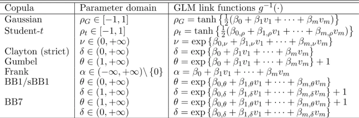
2.1 The link functions for some selected bivariate copulas. The parameter δ

of BB1 copula is [1,+∞), but it reduces to a Clayton copula when δ = 1. Thus, only a range of (1,+∞) is assigned for the parameterδ. For the same reason, a range of (1,+∞) is considered for the parameter θ in the BB7

copula. . . 17

2.2 Degeneration of candidate copulas. . . 20

2.3 The algorithm for estimation of sparse vine-GLM copula models. . . 21

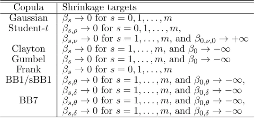
2.4 Shrinkage targets for bivariate copula-GLM. . . 22

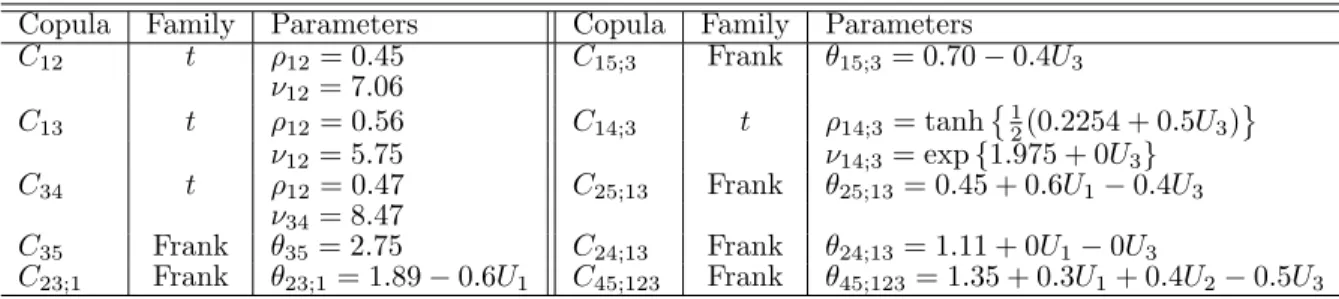
2.5 Families and parameters of the bivariate copulas for vine copula simulation. 23 2.6 Vine-SA copula parameter estimations. . . 24

2.7 Sparse vine-GLM copula estimation. . . 25

2.8 Model selection: vine-SA versus sparse vine-GLM. . . 26

2.9 95% confidence intervals of the GLM coefficients in C14;3. . . 27

2.10 Parameters of simulated standard-GARCH(1,1) with t distributed innova-tion. Here, νi is the degree-of-freedom of a Student-t distribution. . . 28

2.11 VaRα and TVaRα simulated from three models. Numbers in brackets show 95% confidence intervals. . . 29

(12)

2.12 Candidates for the three components in GARCH(1,1)-type models. . . 30

2.13 Fitted marginal distributions for 10TNote, 10Bund, Msci.world, DAX, and S&P 500. . . 31

2.14 Fitted vine-SA and sparse vine-GLM (LASSO) models: tis short for

Student-t. . . 33

2.15 Fitted sparse vine-GLM (SCAD) models. . . 34

2.16 Estimation results of fitting vine-SA, and sparse vine-GLM copulas to the dataset with variables 10TNote, 10Bund, Msci.world, DAX and S&P 500. . 34

2.17 95% confidence intervals of fitted GLM coefficients for C23;4. . . 35

2.18 Ranges of Kendall’s taus of fitted conditional bivariate copulas. . . 36

2.19 Estimation results of fitting sparse vine-GLM copulas, of which calibration functions include second-order terms, to the dataset with variables 10TNote, 10Bund, Msci.world, DAX and S&P 500. . . 36

2.20 Model selection for dataset with 25 out of the Dow 30 companies. . . 38

3.1 Fitted R-squared and Adjusted R-squared for five stock-market indices . . 43

3.2 The algorithm of variable selections for index tracking. . . 53

3.3 In-sample empirical MSE (MSEin) and out-of sample empirical MSE (MSEout). “GCD”

refers to our method using Yanai’s GCD criterion to select stocks. Similarly, “dCor” and “HHG” represent using the distance correlation and HHG test statistics to select stocks respectively. The last column shows published results in [105]. . . 60

3.4 In-sample empirical 95% CVaR (CVaRin) and out-of sample empirical 95% CVaR (CVaRout).

“GCD” refers to our method using Yanai’s GCD criterion to select stocks. Similarly, “dCor” and “HHG” represent using the distance correlation and HHG test statistics to select stocks respectively. Here, “Benchmark” refers to results given by solving (3.9) using the Matlab built-in function “intlinprog”. . . 61

(13)

4.1 In-sample structured (Struc.) MSEs and out-of sample structured MSEs of tracking the Russell 2000 and Russell 3000 by at most 50, 100, and 150 stocks. 86

4.2 In-sample empirical MSE (Emp. MSE), out-of sample empirical MSE, and cross-validation (CV) errors of tracking the Russell 2000 and Russell 3000 by at most 50, 100, and 150 stocks. In the last column,h. is short forhours, and s. is short for seconds. . . 88

5.1 The number of components of synthetic indicies . . . 111

(14)

List of Figures

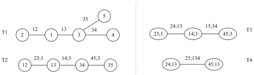
2.1 Tree structure of the true vine copula for simulation studies. . . 23

2.2 Tree structure of the fitted vine-SA and sparse vine-GLM copula. . . 24

2.3 The 95% confidence band of the fitted C14;3’s Kendall’s tau. The dashed

lines indicate the 95% confidence band. The solid curve is the Kendall’s tau of C14;3in the fitted sparse vine-GLM copula, while the dash-dot line is the

Kendall’s tau of C14;3 in the fitted vine-SA copula. The dotted curve is the

Kendall’s tau of the true model. . . 27

2.4 Tree structure of the fitted vine-SA and sparse vine-GLM: nodes 1, 2, 3, 4, and 5 respectively correspond to variables 10TNote, 10Bund, MSCI.world, DAX and S&P 500. Ti stands for the i-th tree, i= 1, . . . ,4.. . . 32

2.5 The 95% confidence band of the fitted C23;4’s Kendall’s tau. The dashed

lines indicate the 95% confidence band. The solid curve is the Kendall’s tau of C23;4in the fitted sparse vine-GLM copula, while the dash-dot line is the

Kendall’s tau of C23;4 in the fitted vine-SA copula. . . 35

4.1 Ranks, by magnitude, of the cross-validation (CV) error, out-of-sample structured (Struc.) MSE, and out-of-sample empirical (Emp.) MSE at different values of λα. . . 85

(15)

5.2 Minimized True Risk vs. Actual Risk, n = 200, #stock=752. . . 109

5.3 Minimized True Risk vs. Actual Risk, n = 450, #stock=2,072. . . 110

5.4 Results of the L1-regularization method to track the Russell 2000 . . . 115

5.5 Tracking portfolio values vs. index level . . . 118

(16)

Chapter 1 Motivations for Topics in this Thesis

Financial institutions usually hold myriad assets, and at the same time they undertake a vast number of risks. In order to achieve excellent business performance, financial insti-tutions need expertise to manage a great number of assets and the exposed risks. This is also a requirement from their stakeholders.

Market regulators require financial institutions to model the dependence structure among their risks. For example, since the second Basel Accord ([13, Part 2]), banks are encouraged to maintain an economic capital which is calculated from their market risk, credit risk, and operational risk. Since each of these three major risks consists of many subcategorized risks, banks usually establish a high-dimensional joint distribution to quantitatively model their risks, and then economic capital is derived from this joint distribution.

From the shareholders’ point of view, financial institutions are expected to increase companies’ values as much as possible. Asset management plays an important role for financial institutions to meet that objective. Among different assets, such as commodities, fixed-income products, equities, real estate, etc., this thesis focuses on equity investment management which is one of the key components of institutional asset management ([89, p.408]). A good equity investment relies on wise decisions on selecting stocks from numer-ousinternational or domestic equities and allocating funds among selected stocks.

(17)

However, it is neither worthwhile nor technically possible for financial institutions to pay detailed attention to each of their risks or each equity in the world. Due to different characteristics of their asset portfolios, financial institutions assign priorities to their major or most risky assets. Traditionally, identifying important risk drivers is based on business savvy, such as experts’ experience and acumen. Nowadays, the information explosion makes these traditional methods too expensive and time-consuming. In response, financial institutions turn to embrace data-driven or quantitative methods ([11]).

This thesis is devoted to establishing sparse models for dependence modelling and port-folio management via data-driven methods. It helps financial institutions to efficiently (in terms of time and accuracy) identify influential dependence structures and select valuable equities in which to invest. More specifically, this thesis is divided into two parts. Chap-ter 2 improves the vine copula, a flexible method to model high-dimensional dependence structures. Chapters3-5focus on constructing tracking portfolios to reproduce returns of stock-market indices, which is a dominant method of passive equity investment strategies ([89, p.410], [108]). In subsequent parts of this thesis, investment only refers to equity investment, unless otherwise stated.

1.1 Sparse models in High-Dimensional Dependence

Modelling

Dependence modelling plays a pivotal role in risk management, for example calculating economic capital. In most cases, the enterprise-level risk is aggregated from numerous dependent risk factors, so that an accurate modelling of the inter-relationship among these risk factors is the key to prudent risk management. The copula method is a popular ap-proach to model dependence ([39]). One of its virtues is to model a joint distribution via two separate steps. The first step determines appropriate marginal distributions. The second step seeks an appropriate copula function to describe the dependence structure. Techniques for bivariate copulas are relatively mature, but high dimensional copulas are still under development. The multivariate Gaussian copula has been widely used in port-folio selection, credit risk management as well as many other applications in finance; see,

(18)

e.g., [25]. Despite its popularity, the Gaussian copula fails to capture some stylized facts of financial data, such as the strong tail dependence or the asymmetric dependence structure ([39]). Other elliptical copulas, particularly the Student-t copula, have been proposed to capture the tail dependence, but they still fail to capture asymmetric dependence struc-tures.

The vine copula ([9], [1]) provides a flexible tool to capture asymmetry and tail depen-dence in modelling multivariate distributions. Nevertheless, its flexibility is achieved at the expense of exponentially increasing the model complexity. To alleviate this issue, the simplifying assumption (SA), which is discussed later in Section 2.2, is commonly adopted in specific applications of vine copula models. In order to relax the SA, Chapter 2 pro-poses generalized linear models (GLMs) to describe parameters in conditional bivariate copulas. In the spirit of the principle of parsimony, a regularization methodology is de-veloped to control the number of parameters, leading to sparse vine copula models. The conventional vine copula with the SA, the proposed GLM-based vine copula and the sparse vine copula are applied to several financial datasets. Empirical results show that proposed models in Chapter 2outperform the one with the SA significantly in terms of the Bayesian information criterion.

1.2 Sparse models in Index Tracking

1.2.1 The Virtue of Index Tracking

In general, investment strategies can be classified as active investment strategies and passive investment strategies. Active fund managers use flexible methods to achieve high returns with low risk. Most passively managed funds, such as index funds and exchange-traded funds, aim at mimicking returns of benchmarked financial-market indices. This strategy is called index tracking. Compared with active investment strategies, passive investment strategies usually deliver higher risk-adjusted returns (in terms of Sharpe ratio or Jensen’s alpha) and charge lower management fees. According to [129, p. 27], the average annual

(19)

management fee for mutual funds is 1.67 percent, while the average is 0.40 percent for exchange-traded funds.

The motivation for passive investment management originates from studies on evaluat-ing mutual fund performance, and dates back to the introduction of Sharpe ratio ([110]) and Jensen’s alpha ([72]). Empirical studies in [110] show that Sharpe ratio of the return of the Dow Jones Industrial Average is higher than the average Sharpe ratio of active mutual fund returns (before transaction costs and management expenses) studied in that paper. The outperformance of stock-market indices is reinforced in [72]. It points out that the average Jensen’s alpha of active managed funds in the U.S. (both before and after transaction costs and management expenses) is negative, when these fund returns are regressed against the S&P 500 return. More granular empirical studies are carried out in [111], which show that the studied actively managed mutual funds fail to deliver significant positive relative returns on average, compared with their benchmark portfolios. According to active managers’ investment style, the benchmark portfolio in [111] is a linear combination of financial indices representing different asset classes.

Even though empirical studies in the 1960s ([110], [72]) point out that stock-market indices beat the majority of active mutual funds in terms of risk-adjusted returns, stock-market indices cannot be used as investment tools. This is because they are only published numbers and do not generate any payoff themselves1_{. But ten years later, index funds came} to the market in the 1970s ([89, p.412]). Empirical studies on the U.S. market in [53] show that (after expense) risk-adjusted returns of index funds tracking the S&P 500 index are higher than the average risk-adjusted return of actively managed mutual funds.

The recent boom in exchange-traded funds (ETFs) also boosts the development of index tracking methods. Due to attractive risk-adjusted returns, low management fees, and transparent objectives (which are simply tracking an index return), ETF has gained increasing popularity since it was first introduced in North America around the early 1990s ([57]). By June 2015, global ETF assets hit US$3 trillion, which has increased by 200% since 2010 ([106], [112]). Thanks to various ETFs tracking different kinds of financial 1_{Even though trading index futures could obtain index returns, but behind index futures stands the} index fund to hedge them.

(20)

market indices, the idea of Sharpe’s benchmark portfolios defined in [111] can be easily realized ([10]).

Index tracking plays an important role for institutional investors. Take pension funds as an example. In 2014, 50.7% of the assets managed by the Canadian Pension Plan was invested passively ([28]), 42.1% of the assets managed by the French Pensions Reserve Fund (Fonds de Reserve Pour Les Retraites) was invested passively in 2013 ([54]), and so was 86.0% of the assets managed by the Janpenese Government Pension Investment Fund in 2013 ([62]).

1.2.2 Constructing Tracking Portfolios via Partial Replication

Index tracking relies on a tracking portfolio to reproduce the return of a benchmark stock-market index. In order to track stock-stock-market indices, a simple strategy is the full repli-cation. Since information of how to calculate a stock-market index is public, at the time of construction a full replication strictly matches its asset weights to those in the index. After that, numbers of asset shares in the full replication hold still until any rebalancing.

After construction, the full replication earning exactly the index return. However, there is always a gap between the terminal wealth of a full-replication and the terminal wealth given the initial wealth (before construction) earns exactly the index return. This gap is caused by the transaction costatconstruction, and a high transaction cost leads to a large gap.

Some ETFs simply apply the full replication to track large-capitalization stock in-dices, such as the methodology of SPDR S&P 500 ETF, which is one of the largest ETFs benchmarked to the S&P 500 index ([119]). Stocks in the S&P 500 index are liquid large-capitalization stocks ([118]), which are easy to trade. Hence, in this case, the tracking gap of a full replication is negligible due to small transaction costs. However, small cap-italization stocks are much less liquid ([80]), so that their high transaction costs usually prevent ETF managers from applying the full replication ([71]). When the full-replication is infeasible, in order to mimic an index return fund managers need to determine in which

(21)

index components to buy and the fund allocation for each selected stock ([71]). In this thesis, this methodology is calledpartial replication, which is the focus of Chapters 3-5.

Chapter 3 focuses on selecting stocks to construct tracking portfolios. Principal com-ponent analysis (PCA) is applied to select stocks via a two-step procedure. In the first step, the index return is expressed as a linear function of principal components (PCs) of stock returns, and a subset of PCs is selected according to Sobol’s total sensitivity index. In the second step, a subset of stocks, which is most similar to those selected PCs, is detected. This similarity is measured by Yanai’s generalized coefficient of determination, the distance correlation, or Heller-Heller-Gorfine test statistics. The weights of selected stocks in the tracking portfolio can be determined by minimizing a specific tracking error. Compared with existing methods, constructing tracking portfolios based on stocks selected by this PCA-based method is more computationally efficient and comparably effective at minimizing the tracking error.

The method of Chapter 3is not so computationally efficient when the number of can-didate stocks is very large. In order to deal with such cases, in Chapter 4 factor models are used to describe stock returns. Under this assumption, the tracking error is partitioned into two parts: one depends on common economic factors, and the other depends on id-iosyncratic risks. According to this partition, a 2-stage method is introduced to construct tracking portfolios by minimizing the tracking error. Stage 1 relies on a mixed-integer lin-ear programming to identify stocks that are able to reduce factors’ impacts on the tracking error, and Stage 2 determines weights of the identified stocks by minimizing the tracking error. This 2-stage method efficiently constructs tracking portfolios benchmarked to indices with thousands of components. It reduces out-of-sample tracking error significantly.

Aiming at reducing the gap between the tracking portfolio terminal wealth and the terminal wealth given the initial wealth (beforeconstruction) earning exactly the index re-turn, Chapter5solves the index tracking problem by repeatedly solving one-period tracking problems. Each one-period tracking strategy is determined by a quadratic optimization with the L1-regularization on asset weights. This formulation addresses the stock

selec-tion and fund allocaselec-tion simultaneously, and it also considers transacselec-tion costs and other practical constraints. Since the true joint distribution of financial returns is usually

(22)

un-known, this chapter solves the one-period tracking problem under empirical distributions. With the L1-regularization on asset weights, the one-period tracking strategy enjoys

per-sistent properties in the high-dimensional setting. More specifically, the variable number d=d(n) =O(nα_{), where}_n_{is the sample size and}_{α >}_{1. Simulation studies are carried out} to support this one-period tracking strategy’s performance with finite samples. Applica-tions on real financial data provide evidence that, in dealing with one-period tracking, this tracking strategy outperforms theLq-penalty tracking method in terms of tracking perfor-mance and computational efficiency. In terms of tracking small-capitalization stock-market indices in multi-period cases, this method outperforms the full-replication strategy.

(23)

Chapter 2 Vine Copula Models with GLM and

Sparsity

2.1 Introduction

Recently, vine copulas have been proposed as powerful alternatives to classical multivariate copulas, such as multivariate elliptical copulas and Archimedean copulas. By decomposing a multivariate copula density into a product of (conditional) bivariate copula densities, the vine copula is flexible enough to capture asymmetric dependence structures as well as strong tail dependence among financial risks. The idea of vine copulas, which dates back to Joe [73] in 1996, is formally introduced by [8,9] as a tool to organize the decomposition of a multivariate copula. Other selected works which have made important contributions to theoretical and practical aspects of vine copulas include [1] which develops a sequen-tial estimation procedure for vine copulas; [32] which studies vine copulas in a Bayesian framework; [122] which develops a time-dependent vine copula model; [113] which proposes a vine-copula GARCH model with dynamic conditional dependence; [96] which discusses the discrete vine copulas; [64] which studies the asymptotic properties of the sequential estimators for vine copula models.

(24)

Because of the complexity of vine copula models, the simplifying assumption (SA) boosts parameter estimations of vine copulas in a more computationally efficient way. It assumes that all bivariate conditional copulas depend on the corresponding conditioning variables only through copula observations, but functional formulas of these bivariate cop-ulas do not depend on the conditioning variables. Though some research works claim that, under certain conditions, the SA will not deteriorate the overall performance of vine copu-las in describing a multivariate joint distribution ([65, 121]), numerical studies conducted by [4] suggest that SA can be too optimistic.

To relax the SA in vine copula modelling, one needs to specify a mechanism to de-scribe the way the conditional bivariate copulas depend on those conditioning variables. One natural way is to model the copula parameters as functions of the conditioning vari-ables. This idea is exploited by [3], where a local polynomial estimation is proposed for conditional copulas; see also [2] and [4]. Moreover, [61] estimates conditional copulas by a purely nonparametric method. While these findings signify the important role of condi-tioning variables, their proposed methods only work for univariate condicondi-tioning variables and extensions to the high dimensional case can be challenging due to the curse of dimen-sionality.

The primary objective of this chapter is to develop a parsimonious vine copula model which relaxes the SA. To accomplish this, generalized linear models (GLM) are proposed for each copula parameter to depend on the corresponding conditioning variables. Such parametric GLM based models provide an explicit way to describe how the dependence in each pair of conditioned variables relies on the conditioning variables, and the resulting models remain computationally efficient for estimation.

The flexibility of the vine copula is achieved at the expense of an exponentially increas-ing complexity of the resultincreas-ing model. Ad-dimensional vine copula consists of d(d−1)/2 (conditional) bivariate copulas and thus contains a large number of parameters for high-dimensional applications. The addition of GLM components inevitably will make a vine copula model even more complex, and thus contradicts to the principle of parsimony in statistical inference, if no further adjustment is provided.

(25)

method to control the number of parameters, leading to sparse vine copula models. The regularization procedure relies on penalized maximum likelihood estimation (MLE) in such a way that the insignificant bivariate dependence diminishes. In this chapter, we use the penalty functions LASSO proposed by Tibshirani ([124]) and SCAD by Fan and Li ([45]), although other penalty functions can similarly be applied.

Our resulting sparse vine copula has the same function as the truncated vine copula introduced by [15], with both aiming to reduce the model complexity while retaining the most significant dependencies in a multivariate distribution. In a truncated vine copula, one needs to determine the level of tree on the vine from which the dependence is negligible and thus it is critical to explore the “significant” tree level. In our sparse vine copula, the model complexity is controlled by the tuning parameter which is associated with the penalty function used in the estimation procedure. In the specific implementation, the selection of tuning parameter can be conducted by cross-validation. As applications, the conventional vine with SA (vine-SA), sparse vine-SA, and sparse GLM-based vine (sparse vine-GLM) copulas are used to model several financial datasets. The results show that our proposed models outperform the vine-SA significantly in terms of the Bayesian information criterion. This chapter proceeds as follows. Section 2.2 provides a brief overview about vine copulas. Section 2.3 introduces our proposed vine-GLM model and the regularization method used for developing the sparse vine copulas. Section 2.4 presents applications of the vine-SA, sparse vine-GLM, and sparse vine-SA models to several financial datasets. Section2.5 concludes the chapter.

2.2 Preliminaries

A copula is a multivariate distribution C with uniformly distributed marginals on (0,1). Sklar’s Theorem (e.g., [94]) states that every multivariate distribution H with univariate marginals F1, . . . , Fd can be written as H(x1, . . . , xd) = C(F1(x1), . . . , Fd(xd)) for some appropriate d-dimensional copula function C. If H is absolutely continuous and strictly increasing with univariate marginal densitiesf1, . . . , fd, the chain rule implies the following

(26)

expression for its joint density function h(x1, . . . , xd) =c(F1(x1), . . . , Fd(xd))· d Y i=1 fi(xi), (2.1)

wherec is the density of the copula C.

Equation (2.1) implies that the dependence structure for a random vector can be iso-lated from its univariate margins, and dependence modelling for a random vector boils down to specifying a joint copula function C (or equivalently copula density c) and the appropriate forms for univariate margins. While the literature on the bivariate copula has proliferated, the research on multivariate copulas is still developing. In particular, the hierarchical copula-based structures have been recently proposed as a flexible alternative to the standard copula model. One of the most promising structures is the regular vine (R-vine) copula, of which the idea is originally proposed by Joe [73] and further explored by [8,9, 30, 84].

An R-vine distribution entails the specification of a number of hierarchical trees where each edge is assigned with a bivariate copula. These bivariate copulas constitute the building blocks of the joint R-vine distribution. According to Definition 4.4 given in [84], an R-vine V on d variables consists of d−1 trees. The w-th tree Tw has nodes Nw and edges Ew, where Ew consists of unordered pairs of Nw with no circle, w = 1, . . . , d −1, satisfying three conditions:

(a) T1 has nodes N1 ={1, . . . , d}and edges E1;

(b) Forw= 2, . . . , d−1,Tw has nodesNw ={Ew−1} and edges Ew;

(c) (proximity condition) For w = 2, . . . , d−1 and {a, b} ∈ Ew with a = {a1, a2} and

b={b1, b2}, it holds that #(a

T

b) = 1.

To construct an R-vine tree with node set N = {N1, . . . , Nd−1} and edge set E = {E1, . . . , Ed−1}, one associates each edge e = {a(e), b(e);D(e)} in Ew with a bivariate copula densityca(e),b(e);D(e), where nodes a(e) and b(e) are called the conditioned set, and

(27)

D(e) is the conditioning set. An R-vine distribution is defined as the distribution of the random vectorX with conditional copula density of Xa(e), Xb(e)

given the variablesXD(e)

specified asca(e),b(e);D(e)for the R-vine trees with node set N and edge setE. XD(e)denotes

the subvector ofX determined by the indices in D(e). Formal definitions for conditioning set and conditioned set are given in Definition 2.2 of [91].

A triplet (F,V,B) is called an R-vine copula specification ifF= (F1, . . . , Fd) is a vector of continuous invertible univariate distribution functions,V is a d-dimensional R-vine and B ={Be : e ∈ Ew, w = 1, . . . , d−1} is a set of copulas with Be being a bivariate copula assigned to an edgee onEw. According to Theorem 4.2 of [84], the joint density h ofX is uniquely determined by an R-vine copula specification as follows:

h(x) = d Y i=1 fi(xi) d−1 Y w=1 Y e∈Ew ca(e),b(e);D(e) F(xa(e)|xD(e)), F(xb(e)|xD(e)) x_D₍_e₎ . (2.2)

Though the realized multivariate densityhis uniquely determined by a given R-vine copula specification, the representation of a multivariate density in terms of R-vine copula speci-fication is not unique. The same multivariate density can be expressed by a large number of different vine copulas with different tree structures and orderings of variables. This follows from the fact that a multivariate distribution can be decomposed into a product of conditional bivariate distributions in a number of distinct ways; see [1] for more details and examples. Indeed, the number of possible representations increases exponentially with the dimension of the copula, among which the C-vine and D-vine structures are two par-ticularly interesting structures commonly studied in the literature. In a C-vine structure, each tree has a root node which is linked to all the other nodes, and in a D-vine structure, nodes in any tree level can at most have two neighbours and thus every tree is flat on the vine.

As mentioned in the first section, the specific application of R-vine copula models is often accompanied with the SA, which simplifies the decomposition for the joint density

(28)

functionh(x) in (2.2) into h(x) = d Y i=1 fi(xi) d−1 Y w=1 Y e∈Ew ca(e),b(e);D(e) F(xa(e)|xD(e)), F(xb(e)|xD(e)) ,

where the original conditional copula density ca(e),b(e)|D(e)(·, ·

x_D₍_e₎) in (2.2) is replaced by

an unconditional copula density.

It follows from the definition that the R-vine copula approach to dependence modelling involves three aspects: (1) selecting vine structure, (2) selecting bivariate copula families, and (3) estimating bivariate copula parameters. The selection of the vine structure is concerned with determining the structure of each tree on the vine. This issue is discussed in detail in [31]. In general, the basic idea is to choose an appropriate weight corresponding to each edge that measures the contribution of the associated bivariate copula to the overall dependency. A tree structure is said to be optimal if it is a maximum spanning tree in that it has the maximum sum of weights. In this chapter, we follow [31] and choose the absolute Kendall’s tau as the weight variable. The maximum spanning tree can be obtained by Prim’s algorithm (e.g., [27]). To determine a bivariate copula on each edge of the tree, it is common to fit the data with a set of bivariate copula candidates and choose the best one according to certain model selection criterion. Many criteria for selecting bivariate copulas in the context of vine copulas are discussed extensively in [16, Section 5.4]. The key findings of the paper are that the Akaike Information Criterion (AIC), which is defined as AIC = 2K−2 ln(L) withK being the number of parameters and Lbeing the likelihood of the model, is found to be a reliable criterion. The AIC has the highest accuracy in the majority of cases, and it is even superior to the blanket goodness-of-fit test. For this reason, this chapter similarly adopts the AIC criterion for selecting the bivariate copulas.

There exist several methods for estimating a copula model. First, the conventional maximum likelihood (ML) method estimates the marginal parameters and the copula parameters simultaneously. In theory, this method gives the most efficient estimators. Nevertheless, it is commonly accompanied with a non-convex optimization over a large dimension set, and thus computationally cumbersome. Second, the so-called inference for margins (IFM) method proposed by [75] first estimates marginal parameters and then

(29)

uses the resulting parameters to estimate the copula parameters. Third, the semipara-metric (SP) estimation proposed by [59] applies univariate empirical distribution functions (EDFs) to generate copula observations and then estimates copula parameters with the generated observations. The second and third methods are a two-step procedure; they sep-arate the estimation of the copula from the univariate marginal distributions, and hence substantially reduce the computation.

In view of the complexity of a vine copula model, a two-step procedure for estimating its parameters seems more computationally tractable. [1] develops a stepwise estimation, which estimates the bivariate copulas on the same tree-level simultaneously and conducts the estimation in a top-down manner. [64] proves that the stepwise estimation is consis-tent and asymptotically normal, given that the copula observations are generated by the univariate EDFs. [1] also proposes a sequential estimation procedure that estimates each pair copula independently. If all the pair copulas do not share any common parameters, the sequential ML estimation is equivalent to the stepwise ML estimation. In this chapter, we will adopt the sequential ML estimation with the IFM method.

2.3 Vine copula with GLM and sparsity

By “vine-GLM copula” we denote as the vine copulas for which the associated conditional copulas depend on conditioning variables only via their parameters, and each copula param-eter is described by a generalized linear model. The specific setup of our vine-GLM copula model is given in subsection 2.3.1, and the procedure for producing a sparse vine-GLM copula model is described in subsection 2.3.2. Subsection 2.3.3 provides some simulation studies to assess the relative efficiency of our proposed GLM-based copula models to other existing copula models.

2.3.1 Conditional copula with GLM

While the copulas on a vine model are all bivariate, we consider a general d-dimensional continuous responseU= (U1, . . . , Ud) and a set of conditioning variablesV = (V1, . . . , Vm).

(30)

H(u1, . . . , ud|v) =CU;V(FU1(u1|v), . . . , FUd(ud|v)|v), (u1, . . . , ud)∈R

d .

Our GLM-based model assumes that the conditional copula depends on the covariates V via the copula parameters only, so that the joint distribution H(u1, . . . , ud|v) admits the following representation

H(u1, . . . , ud|v) = CU;V(FU1|V(u1|v), . . . , FUd|V(ud|v);θ(v)),

whereθ(v) = (θ1(v), . . . , θp(v)) is the conditional copula parameter vector with θj(v) =gj−1(ηj(v)).

Heregj(·) is a link function andηj(·) is a calibration function forj = 1, . . . , p. For univariate v, the parameter functions θ(v) can be estimated by a polynomial of vas proposed by [3] (see also [4] and [2]). In our GLM-based conditional copulas, we consider a linear function forηj(v) with the following form

ηj(v) = β0,j+β1,jv1+· · ·+βm,jvm, for j = 1, . . . , p, (2.3) wherepdenotes the number of parameters in the conditional copula andβj = (β0,j, . . . , βm,j) is a vector of constant coefficients. The above linear calibration function has the capability of capturing the influence of conditioning variables while still ensuring the tractability of the model. To increase the model flexibility, other conditioning variables’ transformations, such as the quadratic term v2

1, . . . , vm2, can be incorporated to the calibration function to capture their nonlinear effects.

Let βj = (β0,j, β1,j, . . . , βm,j) for j = 1, . . . , p, and β = (β1, . . . ,βp) which collects all the parameters in the conditional copula CU;V. Given a sample {(uk,vk), k = 1, . . . , N}

(31)

for (U,V), the conditional copula model with GLM possesses a log-likelihood function of l(β) + N X k=1 d X i=1 log{fUi(ui,k|vk)},

where fUi(ui,k|vk) denotes the conditional density function of the ith marginal for i =

1, . . . , d, l(β) = N X k=1 log cU;V FU1|V(u1,k|vk), . . . , FUd|V(ud,k|vk);θ1(β1,vk), . . . , θp(βp,vk) ,(2.4)

andθj(βj,vk) = gj−1(β0,j+β1,jv1,k+· · ·+βm,jvm,k) forj = 1, . . . , p. In principle, the MLE ofβ can be obtained by maximizingl(β). It is worth noting thatpis usually smaller than or equal to two in most bivariate copulas which are usually applied in vine copula models. Each copula parameter has a specific domain and this implies that the link function is supposed to be determined according to the same domain. Many popular bivariate copulas, as well as their parameter domains, can be found in [94] and [74]. Table 2.1 shows the choices of the link functions for the bivariate copulas that we will consider in our simulation studies and real data examples. Recall that Gaussian and Frank copulas are symmetric but without tail dependence. The Student-t copula is a tail dependent symmetric copula. Clayton and Gumbel copulas have either lower or upper tail dependence. Following [95], we also consider BB1, survival BB1(sBB1), and BB7 copulas, which exhibit asymmetric tail dependence.

2.3.2 Sparse vine copula

Our proposed vine-GLM copula suffers from an over-fitting problem, since it has more parameters than SA-based vine copulas. In order to ensure the model complexity is kept at a reasonable level while still providing flexible dependence modelling structures, this subsection describes how sparsity can be introduced to our proposed vine-GLM copulas to attain these tradeoffs. Recall that the truncated vine copula of [15] is motivated by the

(32)

Copula Parameter domain GLM link functionsg−1(·) Gaussian ρG∈[−1,1] ρG = tanh ₁ 2(β0+β1v1+· · ·+βmvm) Student-t ρt∈[−1,1] ρt= tanh ₁ 2(β0,ρ+β1,ρv1+· · ·+βm,ρvm) ν ∈(0,+∞) ν = exp{β0,ν+β1,νv1+· · ·+βm,νvm}

Clayton (strict) δ ∈(0,+∞) δ= exp{β0+β1v1+· · ·+βmvm}

Gumbel θ∈(1,+∞) θ= exp{β0+β1v1+· · ·+βmvm}+ 1 Frank α∈(−∞,+∞)\ {0} α=β0+β1v1+· · ·+βmvm BB1/sBB1 θ∈(0,+∞) θ= exp{β0,θ +β1,θv1+· · ·+βm,θvm} δ ∈(1,+∞) δ= exp{β0,δ+β1,δv1+· · ·+βm,δvm}+ 1 BB7 θ∈(1,+∞) θ= exp{β0,θ +β1,θv1+· · ·+βm,θvm}+ 1 δ ∈(0,+∞) δ= exp{β0,δ+β1,δv1+· · ·+βm,δvm}

Table 2.1: The link functions for some selected bivariate copulas. The parameterδ of BB1 copula is [1,+∞), but it reduces to a Clayton copula when δ = 1. Thus, only a range of (1,+∞) is assigned for the parameter δ. For the same reason, a range of (1,+∞) is considered for the parameterθ in the BB7 copula.

empirical observation that the bottom trees on a vine copula model are often negligible in terms of their impact on dependence. This suggests that we can determine the “significant” tree level below which independence can be assumed.

In contrast, our sparse vine copula does not simply focus on these less significant bottom trees. Instead, it shrinks all the “insignificant” bivariate copulas on each tree-level to independent copulas, and the determination of such “insignificance” bivariate copulas is automatically carried out by a penalized estimation procedure.

The sequential estimation procedure proposed by [1] will similarly be used to de-velop our sparse vine copula model. The procedure estimates each bivariate copula in-dividually. Let {(U1i, U2i), i = 1,2, . . . , N} be independent and identically distributed (i.i.d.) observations of a bivariate copula C(u1, u2;θ) with copula density c(u1, u2;θ),

whereθ = (θ1, . . . , θd) is the vector of copula parameters. The penalized MLE is given by ˆ θ = arg max θ ( _N X k=1 `(U1k, U2k;θ)−N d X j=1 p(θj) ) , (2.5)

(33)

Note that the above penalty functionp(θj) is used to “detect” the insignificant parameter by shrinking the estimatorθb_j to zero for each insignificant parameterθ_j in a linear model.

Equivalently, if the penalty function is expressed as p(θj −θ˜j) for some target value ˜θj, then the estimatorθb_j is shrunk to ˜θ_j.

In our numerical examples, we will use the LASSO and SCAD penalties, which are two of the most popular penalty functions in the statistical literature. The LASSO penalty is introduced by [124] for developing sparse linear regression models in a high dimensional setting. Its expression is given by

pL(θj) =λL|θj|,

where the tuning parameterλL>0 is imposed to control the degree to which the estimator is shrunk to zero. The SCAD penalty, which is proposed by [45], has the form

pS(θj) =          λS|θj|, |θj| ≤λS, −(θ2 j −2aSλS|θj|+λ2S)/[2(aS−1)], λS <|θj| ≤aSλS, (aS+ 1)λ2S/2, |θj|> aSλS, (2.6)

whereλS and aS are two tuning parameters with λS >0 andaS >2.

According to [45], LASSO is better than SCAD in situations where there is too much randomness associated with the true model, while SCAD-penalized MLEs are less biased. The SCAD possesses the so-called oracle property, which roughly says that the penalized MLEs work as well as if the correct submodel were known in advance. A comprehensive review of the commonly-used penalty functions is provided in [50]. It is also worth noting that the penalized MLEs can be asymptotically normal under certain conditions as illus-trated by [47]. However, in general the asymptotic normality does not apply (see [98]) and hence in our application, we will use the bootstrap method to construct the confidence intervals for the estimated parameters.

The efficiency of the penalized estimator critically depends on the choice of the tuning parameter in a penalty function since it controls the severity of the shrinkage. For a specific

(34)

application, the tuning parameters are usually determined by a cross-validation procedure, nevertheless [45] recommendsaS = 3.7 for the SCAD penalty. In our numerical examples, we have conducted additional studies to infer the appropriate value ofaS and we similarly conclude the appropriateness of settingaS to 3.7. For this reason, we will continue to use this value for our subsequent numerical work. For other tuning parameters λS or λL, we follow [128] and choose the tuning parameter which gives the best Bayesian information criterion (BIC) for the model. The BIC is computed by BIC =Kln(N)−2 ln(L), where N is the sample size, K is the number of parameters, and L is the likelihood. The BIC rule leads to a more sparse structure than the general cross-validation procedure does. As argued in [128], the general cross-validation procedure is not able to satisfactorily select the tuning parameter while the BIC-based tuning parameter is able to identify the true model consistently. For our implementations, we first conduct some pre-analysis to empirically determine the plausible ranges of the tuning parameters. Then, we obtain the penalized MLEs corresponding to each of a set of selected candidate values of λS or λL, which will be clearly specified in each of the subsequent numerical studies. Finally, we choose λS or λL that gives the best BIC. For a vine copula in a large dimension, choosing the set of tuning parameters for each bivariate copula can be computationally intensive. A sub-optimal solution is to consistently use the same set of tuning parameters for all the bivariate copulas on the same level of tree.

Table2.2(also see Table2.1) displays eight possible bivariate copulas which will be used to develop sparse-based vine copulas in our subsequent numerical studies. While these are not the exhaustive list of bivariate copulas, they are sufficiently representative in that they exhibit distinct distributional shapes in terms of tail dependence and asymmetry. Table2.2

also gives the situation under which the copula degenerates to the independence structure. For example, when the target value of a copula parameter is zero, such as the Gaussian copula’sρ and Clayton copula’sδ, the penalty term in the log-likelihood objective of (2.5) is simply p(θj). When the target value of a parameter is one, such as the BB1 copula’s δ and Gumbel’s θ, the penalty term is replaced by p(θj −1). For the Student-t copula, the target value ofν is set to 31, a value which is large enough for the Student-t copula to be close to a Gaussian copula.

(35)

Copula Degeneration

Student-t Student tcopula → Gaussian copula, asν →+∞.

Gaussian Gaussian copula→ independence copula, as ρG →0.

Clayton Clayton copula → independence copula, as δ→0.

Gumbel Gumbel copula → independence copula, as θ→1.

Frank Frank copula → independence copula, as α→0.

BB1 BB1 copula → Clayton copula, asδ→1.

sBB1 sBB1 copula→ independence copula, as θ→0 andδ→1.

BB7 BB7 copula → Clayton copula, asθ→1.

Table 2.2: Degeneration of candidate copulas.

vine-GLM copula models. As we have pointed out in Section 2.2, we use the absolute Kendall’s tau as the weight measure and apply the Prim’s algorithm to obtain the max-imum spanning tree at each level on the vine. Given copula observations, we apply the method given in [58] to test the independence. If the observations reject the independence assumption, we apply the AIC criterion to choose the best bivariate copula from the eight candidates in Table2.2for each edge of the tree, and simultaneously obtain the estimation for each selected bivariate copula by the penalized MLE procedure as outlined above.

Note that the algorithm also applies the penalized estimation scheme to a vine-GLM copula model. We continue to rely on the AIC rule for the bivariate copula selection. To compute the value of AIC, we have to estimate each candidate bivariate copula on each edge with a GLM specification, and maximize a log-likelihood with an expression similar to l(β) given in (2.4). When the penalized estimation is applied to a vine-GLM copula model, leading to a sparse vine-GLM copula, we have two levels of shrinkage. First, we target to shrink those insignificant coefficientsβs for s= 1, . . . , m in the GLM to be zeros to reduce model complexity. Second, given that all the coefficients βs for s = 1, . . . , m are indeed zeros, the intercept coefficient β0 in the GLM is expected to be shrunk to a

corresponding target so that the resulting copula parameter is attracted to a boundary value (see Table 2.2) and the underlying bivariate copula reduces to be an independent one. The specific shrinkage rule for each conditional bivariate copula-GLM is described in Table 2.4. In the table, a target value of β0 for quite many bivariate copulas to reduce

to the independence copula is −∞. In our specific implementation, we replace the target value of−∞ by log(0.001). Similarly, for the degrees of freedom in the Student-t copula,

(36)

we replace the target value of +∞ by log(31). 1: Inputd-dimensional data.

2: Generate copula observations

3: For w= 1, . . . , d−1do

4: Check for proximity condition.

5: Compute empirical Kendall’s tau matrix. 6: Search for the maximum spanning tree.

7: Foreach bivariate copula in thew-th tree leveldo 8: If tested to be independent, go to Step 16.

9: Else try a certain bivariate copula family in Table 1. 10: ForλL (orλS) in candidate collectionsdo

11: Estimate pair copula parameters (or GLM coefficients) by the LASSO/SCAD estimators. 12: If possible, decay pair copulas according to the penalized MLEs.

13: End for

14: Chooseλwith the lowest BIC, take corresponding penalized MLEs as the final estimation, and compute AIC.

15: Ifall copula families have been tried, choose the one with lowest AIC,else go to Step 9. 16: End for

17: Compute pseudo observations. 18:End for

19: Return the density of the sparse vine-GLM specification.

Table 2.3: The algorithm for estimation of sparse vine-GLM copula models.

2.3.3 Simulation studies

In order to assess the efficiency of the proposed GLM-based sparse vine copula relative to the SA-based vine copula, we consider the following carefully crafted experiments.

First we assume that the true underlying multivariate distribution is given by a five-dimensional vine copula C with the corresponding tree structure depicted in Figure 2.1

and the bivariate copula families together with their parameters as shown in Table 2.5. Note that the bivariate copulas of the above vine copula comprise of Student-tcopulas and Frank copulas. This is motivated by their ease in generating the random samples. The

(37)

Copula Shrinkage targets

Gaussian βs→0 for s= 0,1, . . . , m

Student-t βs,ρ→0 for s= 0,1, . . . , m,

βs,ν →0 for s= 1, . . . , m, and β0,ν,0 →+∞

Clayton βs→0 for s= 1, . . . , m, and β0 → −∞

Gumbel βs→0 for s= 1, . . . , m, and β0 → −∞

Frank βs→0 for s= 0,1, . . . , m

BB1/sBB1 βs,θ →0 fors= 1, . . . , m, and β0,θ → −∞,

βs,δ →0 for s= 1, . . . , m, andβ0,δ → −∞

BB7 βs,θ →0 fors= 1, . . . , m, and β0,θ → −∞,

βs,δ →0 for s= 1, . . . , m, andβ0,δ → −∞

Table 2.4: Shrinkage targets for bivariate copula-GLM.

joint copula density for (U1,· · · , U5), as a result, has the following representation:

c(u1, . . . , u4) = c12(u1, u2)c13(u1, u3)c34(u3, u4)c35(u3, u5) ×c23;1 F2|1(u2|u1), F3|1(u3|u1)|u1 c14;3 F1|3(u1|u3), F4|3(u4|u3)|u3 ×c15;3 F1|3(u1|u3), F5|3(u5|u3)|u3 ×c24;13 F2|13(u2|u1, u3), F4|13(u4|u1, u3)|u1, u3 ×c25;13 F2|13(u2|u1, u3), F5|13(u5|u1, u3)|u1, u3 ×c45;123 F4|123(u4|u1, u2, u3), F5|13(u5|u1, u2, u3)|u1, u2, u3 . (2.7)

A controlled data set of size 10,000 is then constructed by simulating the required samples from the above copula density. Using the procedure as outlined earlier, the SA-based vine copulas and GLM-SA-based vine copulas are fitted to the controlled data set. Since we have complete information about the controlled data set, the efficiency of the fit can easily be gauged. The fitted tree structure is shown in Figure 2.2 and the fitted bivariate copulas (together with their fitted parameter values) are given in Tables 2.6 and

2.7 for the vine-SA model and the sparse vine-GLM model, respectively. The candidate bivariate copulas used in the estimation procedure correspond to those in Table2.1. Note that for the GLM-based copulas, we consider both LASSO and SCAD penalty functions. Furthermore, our pre-analysis on possible tuning parameters indicates that the plausible range for the LASSO’s tuning parameterλLis [10−6,10−4] while SCAD’s tuning parameter

(38)

λS is [0.05,0.10]. After that, ten candidates of tuning parameters are evenly selected from the respective ranges to produce ten fitted GLM-based sparse vine-copulas associated with each penalty function. The fitted set that yields the best BIC is the one that is reported in Table 2.7. 2 4 5 3 1 12 15;3 23;1 34 35 13 34 35 13 12 14;3 15;3 23;1 14;3 25;13 24;13 25;13 45;123 24;13 T1 T2 T3 T4

Figure 2.1: Tree structure of the true vine copula for simulation studies. Copula Family Parameters Copula Family Parameters

C12 t ρ12= 0.45 C15;3 Frank θ15;3 = 0.70−0.4U3 ν12= 7.06 C13 t ρ12= 0.56 C14;3 t ρ14;3= tanh 1 2(0.2254 + 0.5U3) ν12= 5.75 ν14;3= exp{1.975 + 0U3} C34 t ρ12= 0.47 C25;13 Frank θ25;13 = 0.45 + 0.6U1−0.4U3 ν34= 8.47 C35 Frank θ35= 2.75 C24;13 Frank θ24;13 = 1.11 + 0U1−0U3 C23;1 Frank θ23;1= 1.89−0.6U1 C45;123 Frank θ45;123 = 1.35 + 0.3U1+ 0.4U2−0.5U3 Table 2.5: Families and parameters of the bivariate copulas for vine copula simulation.

Based on the fitted results, we make the following remarks:

• It is of interest to note that all the three fitted models consistently yield the same tree structure as shown in Figure 2.2. The estimated tree structure, however, deviates from the true tree structure as depicted in Figure 2.1. The misspecification is not surprising since the method used to determine tree structures is not guaranteed to provide the true structure.

• All the three fitted models have the identical first tree in terms of the same bivariate copula families (compare Table 2.5 to Tables 2.6 and 2.7). Furthermore, the fitted parameter values are very close to their true counterparts.

(39)

2 4 5 3 1 12 45;3 23;1 34 35 13 34 35 13 12 14;3 23;1 14;3 45;3 24;13 15;34 24;13 25;134 45;13 T1 T2 T3 T4

Figure 2.2: Tree structure of the fitted vine-SA and sparse vine-GLM copula.

Copula Family Parameters Copula Family Parameters

C12 t ρˆ12= 0.4460 C14;3 t ρˆ14;3= 0.2417 ˆ ν12= 7.4391 νˆ14;3= 7.0054 C13 t ρˆ13= 0.5482 C45;3 Frank θˆ45|3 = 1.5908 ˆ ν13= 5.3925 C34 t ρˆ12= 0.4563 C24;13 Frank θˆ24;13= 1.0638 ˆ ν34= 8.0040 C35 Frank θˆ35= 2.7410 C15;34 Frank θˆ15;34= 0.0472 C23;1 Frank θˆ23;1= 1.5196 C25;134 Frank θˆ25;134= 0.3474

Table 2.6: Vine-SA copula parameter estimations.

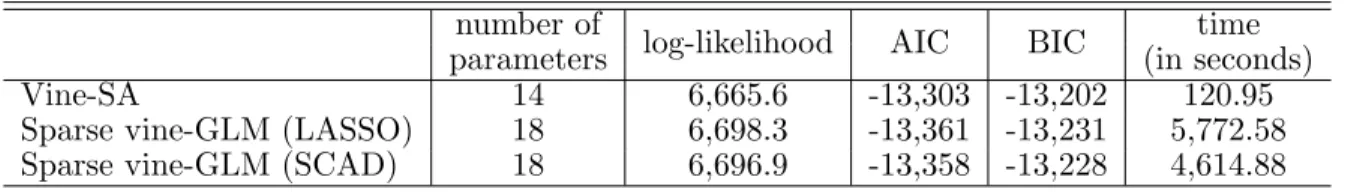
The criterion based on either AIC or BIC clearly supports the superiority of the GLM-based sparse vine copulas over the SA-GLM-based vine copulas. According to [19], a difference in AIC larger than 10 is a significant support in selecting better models, and a difference between 4 and 7 provides considerable support. [79] shows that a difference in BIC larger than 5 is significant. Therefore, Table 2.8, which reports the AICs and BICs of the three fitted models, shows that both the AIC and BIC prefer our proposed model significantly to the vine-SA model. The key difference between AIC and BIC is that the latter penalizes the size of the sample data so that the larger the sample size, the heavier the penalty. They disagree when AIC chooses a more complex model than BIC does. We use AIC to select pair copulas, as a bivariate copula usually has at most two parameters. But in high-dimensional cases, such as selecting vine copula models, we focus on BIC especially when AIC and BIC prefer different models, because BIC favours a parsimonious model more than AIC in high dimensions, while AIC is likely to lead to an overfitted model. According to [34], BIC is a consistent selector that will select the true model with probability of 1 as

(40)

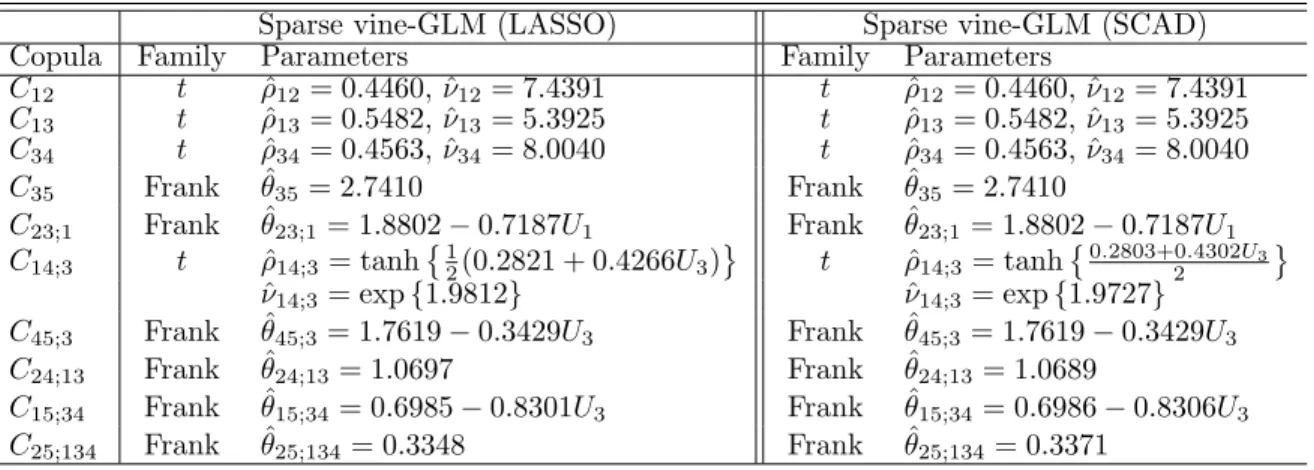
Sparse vine-GLM (LASSO) Sparse vine-GLM (SCAD) Copula Family Parameters Family Parameters

C12 t ρˆ12= 0.4460, ˆν12= 7.4391 t ρˆ12= 0.4460, ˆν12= 7.4391 C13 t ρˆ13= 0.5482, ˆν13= 5.3925 t ρˆ13= 0.5482, ˆν13= 5.3925 C34 t ρˆ34= 0.4563, ˆν34= 8.0040 t ρˆ34= 0.4563, ˆν34= 8.0040 C35 Frank θˆ35= 2.7410 Frank θˆ35= 2.7410 C23;1 Frank θˆ23;1 = 1.8802−0.7187U1 Frank θˆ23;1= 1.8802−0.7187U1 C14;3 t ρˆ14;3= tanh 1 2(0.2821 + 0.4266U3) t ρˆ14;3= tanh 0.2803+0.4302U3 2 ˆ ν14;3= exp{1.9812} νˆ14;3 = exp{1.9727} C45;3 Frank θˆ45;3 = 1.7619−0.3429U3 Frank θˆ45;3= 1.7619−0.3429U3 C24;13 Frank θˆ24;13= 1.0697 Frank θˆ24;13= 1.0689 C15;34 Frank θˆ15;34= 0.6985−0.8301U3 Frank θˆ15;34= 0.6986−0.8306U3 C25;134 Frank θˆ25;134= 0.3348 Frank θˆ25;134= 0.3371 Table 2.7: Sparse vine-GLM copula estimation.

the sample size goes to infinity, while AIC might not. The legitimacy of the BIC has also been justified by [56].

Table 2.8 also shows the elapsed time of fitting the vine-SA, sparse vine-GLM with LASSO and SCAD penalties to the simulated data. All fitting procedures in this chapter are carried out with MATLAB (Version R2014a) on a PC with Intel Core i5-3210M CPU at 2.5GHz and 6.00GB memory. Fitting sparse vine-GLM models needs more time than fitting vine-SA, because 1)starting from the second tree GLM introduces more parameters to each bivariate copula, and 2) each copula type is fitted 10 times for every bivariate copula due to ten tuning parameter candidates.

In the rest of the section, we shall only focus on the LASSO penalty for fitting the sparse vine-GLM model, as the results with the SCAD are similar and almost all the same comments can be applied similarly. To provide additional insight on the fitted GLM-based sparse vine copula model, let us now focus on the fitted bivariate copula C14;3 using the

LASSO penalty. Similar comments apply to that based on the SCAD penalty.

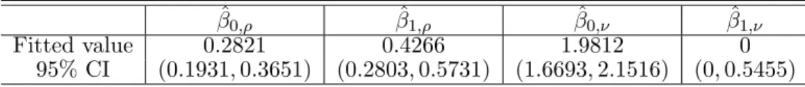
We first examine the accuracy of the fitted parameter values relative to the true pa-rameter values. This can be accomplished by examining the confidence intervals of the fitted values. As asymptotic normality may not apply to the present model, we resort to the bootstrap method to construct the required confidence intervals. We resample the

(41)

original controlled data set with replacement and estimate the copula parameters based on the resampled data. We repeat this procedure 1,000 times so as to obtain 1,000 sets of parameter estimators. We view these 1,000 estimators as sample of the parameter es-timators and use their 2.5% and 97.5% empirical quantiles to construct a 95% confidence interval. The results are shown in Table 2.9. Comparing to their true parameter values (see Table 2.5), it is reassuring that the constructed 95% confidence intervals contain the true parameter values.

Next, we are interested in the Kendall’s tau of the bivariate copulaC14;3. More

specif-ically, we are interested in how the Kendall’s tau of variables U1 and U4 evolves along

with the value of U3 over the whole interval (0,1) since for such a conditional copula, the

value of Kendall’s tau depends on the value of the conditioning variableU3. The Kendall’s

tau of the true model for each given value of U3 can be computed based on the specified

copula family and the GLM models for its parameters given in Table 2.5. The results are demonstrated by the dotted curve in Figure 2.3. To develop an estimate for such a true curve of Kendall’s tau, we first fit a sparse vine-GLM model using the previously constructed data set and then compute the Kendall’s tau based on the fitted parameter values for each value of U3 over the interval (0,1). The results are demonstrated by the

solid curve in Figure 2.3, along with the confidence bands which are similarly estimated using the bootstrap method. It is again reassuring that the true Kendall’s tau falls in the 95% confidence band estimated with a sparse vine-GLM copula. The graph also reports the estimated Kendall’s tau based on a vine-SA copula. In this case, the Kendall’s tau is a constant and is illustrated by the dash-dot flat line since the conditional copula does not depend on the conditioning variable U3.

number of

log-likelihood AIC BIC time

parameters (in seconds)

Vine-SA 14 6,665.6 -13,303 -13,202 120.95

Sparse vine-GLM (LASSO) 18 6,698.3 -13,361 -13,231 5,772.58

Sparse vine-GLM (SCAD) 18 6,696.9 -13,358 -13,228 4,614.88

Table 2.8: Model selection: vine-SA versus sparse vine-GLM.

(42)

ˆ

β0,ρ βˆ1,ρ βˆ0,ν βˆ1,ν

Fitted value 0.2821 0.4266 1.9812 0

95% CI (0.1931,0.3651) (0.2803,0.5731) (1.6693,2.1516) (0,0.5455)

Table 2.9: 95% confidence intervals of the GLM coefficients in C14;3.

0 0.2 0.4 0.6 0.8 1 0.06 0.08 0.1 0.12 0.14 0.16 0.18 0.2 0.22 0.24 0.26 U 3 Kendall tau

Figure 2.3: The 95% confidence band of the fittedC14;3’s Kendall’s tau. The dashed lines

indicate the 95% confidence band. The solid curve is the Kendall’s tau of C14;3in the fitted

sparse vine-GLM copula, while the dash-dot line is the Kendall’s tau of C14;3 in the fitted

vine-SA copula. The dotted curve is the Kendall’s tau of the true model.

In particular, we are interested in Value-at-Risk (VaR) and Tail Value-at-Risk (TVaR). The VaR and TVaR of a profit-and-loss random variable S at a confidence level α for 0 < α < 1 are defined as VaRα(S) = inf{s ∈ R : Pr(S ≤ s) ≥ α} and TVaRα(S) =

E[S|S ≤VaRα(S)], respectively.

Suppose that a dollar is invested in each of five (correlated) assets at time t−1 and that rt,q denotes the daily log-return of the q-th asset at time t, q = 1, . . . ,5. Then, the one-day profit-and-loss variable at time t of the investment portfolio is given by

St =

5

X

q=1

ert,q ₋₅_. _(2.8)

We are concerned with estimating the VaR and TVaR of the one-day profit-and-loss variable St based on vine-SA and sparse vine-GLM (LASSO) copula models.

(43)

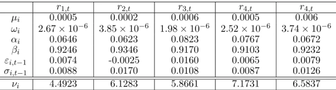
The Generalized AutoRegressive Conditional Heteroskedasticity (GARCH) model is widely applied for modelling the log-return data of financial time series. In our simulation studies, each of the five daily log-return variablesrt,q is assumed to follow a GARCH (1,1) model

rt,q =µq+εt,q, εt,q =σt,qzt,q, σt,q2 =ωq+αqε2t−1,q +βqσt2−1,q, for q= 1, . . . ,5, (2.9) with parameter values given in Table2.10, where each innovation zq,t is assumed to have a Student-t distribution with degree of freedom specified in the table as well. We further as-sume that the innovation vector (z1,t, z2,t, z3,t, z4,t, z5,t) is subject to a dependence structure governed by the copula density (2.7) with the tree structure and bivariate copulas (both families and parameters) specified in Figure2.1 and Table 2.5 respectively.

r1,t r2,t r3,t r4,t r4,t µi 0.0005 0.0002 0.0006 0.0005 0.006 ωi 2.67×10−6 3.85×10−6 1.98×10−6 2.52×10−6 3.74×10−6 αi 0.0646 0.0623 0.0823 0.0767 0.0672 βi 0.9246 0.9346 0.9170 0.9103 0.9232 εi,t−1 0.0074 -0.0025 0.0160 0.0065 0.0079 σi,t−1 0.0088 0.0170 0.0108 0.0087 0.0126 νi 4.4923 6.1283 5.8661 7.1731 6.5837

Table 2.10: Parameters of simulated standard-GARCH(1,1) witht distributed innovation. Here, νi is the degree-of-freedom of a Student-t distribution.

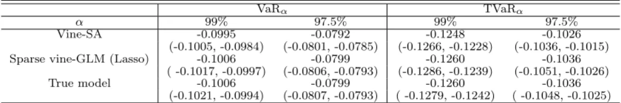
In order to evaluate the VaR and TVaR of the portfolio at time t, we simulate 100,000 samples of the log-return vector (r1,t, . . . , r5,t) from model (2.9) to obtain 100,000 samples of the profit-and-loss variable St. The VaR and TVaR are then computed from these samples assuming confidence levels of 97.5% and 99%, respectively. We replicate the simulation 50 times independently and compute the average and standard deviation over these 50 estimations to produce conference intervals of the risk measures. The resulting average and the 95% confidence interval are assumed to be the correct values and are reported under the row labelled “True model” in Table 2.11. These values will be the benchmarks for the estimated VaR and TVaR from both the fitted vine-SA and sparse vine-GLM (with LASSO) models.

(44)

VaRα TVaRα

α 99% 97.5% 99% 97.5%

Vine-SA -0.0995 -0.0792 -0.1248 -0.1026

(-0.1005, -0.0984) (-0.0801, -0.0785) (-0.1266, -0.1228) (-0.1036, -0.1015)

Sparse vine-GLM (Lasso) -0.1006 -0.0799 -0.1260 -0.1036

( -0.1017, -0.0997) (-0.0806, -0.0793) (-0.1286, -0.1239) (-0.1051, -0.1026)

True model -0.1006 -0.0799 -0.1260 -0.1036

(-0.1021, -0.0994) (-0.0807, -0.0793) ( -0.1279, -0.1242) ( -0.1048, -0.1025)

Table 2.11: VaRα and TVaRα simulated from three models. Numbers in brackets show 95% confidence intervals.

An immediate conclusion that can be drawn from Table 2.11 is that the estimated VaR and TVaR from the sparse vine-GLM are much closer to the true values than the corresponding estimates from the vine-SA. More severely, the estimated risk measures from the vine-SA are much less negative than the corresponding true values. This implies that risk measures from the vine-SA consistently underestimate the underlying risk.

2.4 Application to financial data

In this section, we apply our proposed vine copula models to daily log-returns of some finan-cial assets and compare their performance to the vine-SA copula model. We consistently use the two-step method of IFM for the estimation. The first step focuses on modelling the (parametric) univariate marginal distribution. By using the results from the first step, the second step generates the resulting vine copula observations and estimates the vine copula using the sequential estimation procedure. The general procedure of estimating the univariate marginal distributions is described in the following subsection. Subsection2.4.2

considers an application of the sparse vine-GLM copula model to a 5-dimensional financial dataset. The impact of sparsity on vine-SA copula is illustrated in subsection 2.4.3.

2.4.1 Estimating univariate marginals

Determining proper univariate marginal distributions is the first and also a critical step in the IFM method since any fitting error will be carried over to fitting copulas in the second