Permeability estimation from time-lapse seismic data for updating the flow-simulation model

(1)

Permeability Estimation From

Time-Lapse Seismic Data For Updating the

Flow-Simulation Model

Mehdi Paydayesh

A Thesis Submitted for the Degree of Doctor of Philosophy,

Institute of Petroleum Engineering,

Heriot-Watt University, Edinburgh, United Kingdom.

April 2010

The copyright in this thesis is owned by the author. Any quotation from the thesis or use of any of the information contained in it must acknowledge this thesis as the source of

(2)

ABSTRACT

The key to increasing reservoir recovery is to provide accurate estimates of the permeable pathways (permeability, transmissibility) and the transmissibility of the barriers that control reservoir heterogeneity. The reservoir-engineering techniques (such as well testing, well logging and production data) supply the estimate of these properties in the reservoir region which is limited to well locations. Providing estimates of the permeability in the reservoir rocks located between the wells is the holy grail of reservoir engineering for history matching. Compared with all other engineering techniques, 4D seismic could play a unique role in providing the property of the reservoir at a good spatial coverage. In this thesis, the estimation of permeability, transmissibility, and the transmissibility multiplier, using 4D seismic, is addressed.

First, current methodologies for permeability estimation were applied in synthetic and field examples. Based on the investigations performed, the permeability-estimation method was modified and adjusted to produce an improved result. Consequently, the estimates of permeability provided an introduction to the fast-track history-matching method. The proposed history-matching technique implies a simple and practical approach for quickly updating the simulation to improve the history-matching in the model. In following, the assessment of the uncertainties associated with the permeability estimation that involves using a variety of different attributes, using different time-lapse surveys, tuning effects and method assumptions, were performed. The uncertainties were tackled by addressing these issues; thus, the permeability result was further enhanced, and the uncertainty associated with the estimates was quantified. Next, the relationships between the quantitative estimates of connectivity and the 4D seismic signal were established. Two types of connectivity assessments using 4D seismic (hydraulic sand connectivity and barrier connectivity) were proposed, depending on the fact that 4D-seismic information is either pressure- or saturation-dominant. Accordingly, two types of attributes were introduced, the seismic connectivity attribute (SCA) and the Laplacian attribute. When applied to the Schiehallion field data, an interpretation approach is used to interpret pressure- and saturation-anomalies in frequent time-lapse seismic, using all available sources of data. Following this, a pressure-anomaly map is utilized for locating faults and compartments

(3)

(using the Laplacian attribute), and a saturation-anomaly map is used to calculate the SCA. New approaches were chosen for estimating transmissibility and transmissibility multipliers, based on proposed attributes extracted from 4D seismic.

(4)

(5)

(6)

ACKNOWLEDGMENTS

Part of my journey is coming to an end. These have been the best and most challenging years of my life so far. I am indebted to the many people who have been instrumental in the successful completion of my research. To begin, I will thank God for having made everything possible – by giving me the strength and courage to accomplish this work.

I would like to express my heartfelt thanks to my supervisor, Professor Colin MacBeth, for the extensive time that he spent guiding my research. He was always accessible, and constantly provided insightful reviews and timely responses throughout the various stages of this work.

Special thanks should go to Dr Xuri Huang and Dr Asghar Shams for investing their time in reading and evaluating my thesis. I am grateful that, despite their many other commitments, they agreed to become members of the examining committee.

I would like to thank Dr Rossmary Villegas for her collaboration on the history-matching part of this thesis. I also acknowledge the Schiehallion field partners (BP, Shell, Hess, Statoil (UK) Ltd, Murphy Petroleum Ltd, and OMV) for providing the data, and for giving me permission to publish them. I am also grateful to the sponsors of the Edinburgh Time-Lapse Project, Phase III (BG, BP, Chevron, ConocoPhillips, EnCana, ExxonMobil, Hess, Ikon Science, Landmark, Maersk, Marathon, NORSAR, Petrobras, Shell, Statoil (UK) Ltd, Total, and Woodside) for their financial support of this research.

As a recipient of the BP/Ian Jack Scholarship, I would like to express my sincere thanks to the SEG Foundation Scholarship Program, and especially to Ian Jack for his encouraging and motivating comments on my work.

I am indebted to my fellow office-mates, Hamed Amini, Amran Benguigui, Nuri Edriz, Yesser Hajnasser, Dr Weisheng He, Nader Kooli and Valeriy Rukavishnikov, for providing an inspiring and enjoyable environment in which to learn and grow. During these memorable years, we spent most of our time together, like a family, sharing our knowledge, joy, happiness and sadness. I am also grateful to all the members of the Reservoir Geophysics group: Fabian Domes, Reza Falahat, Ilya Fursov, Alejandro

(7)

Garcia, Yi Huang and Karl Stephen. I am thankful to all the staff at the Institute of Petroleum Engineering, in particular the computer-support staff, for their continuous support.

For my parents‟ continued love and encouragement I can never thank them enough. They have been my inspiration throughout this endeavour. Mere words fail to express my appreciation to my wife, Raheel, for her endless patience, love and encouragement that buoyed me up throughout my PhD. This thesis would not have been possible without her invaluable, constant support. I also wish to acknowledge my sisters and family-in-law for their prayers and support.

(8)

LIST OF TABLES

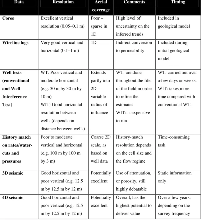
Table 1.1: Comparison of the different tools used for the measurement of permeability ... 12

Table 2.1: Captured signatures of permeability in absolute values of Laplacian used in the Seis2perm method, based on modelling for the various generated permeabilities . . 36

Table 3.1: Comparison between the seismic matching and the fast-track history-matching approaches. ... 75

Table 4.1: The range of attributes and their descriptions. ... 80

Table 4.2: Cp and Csconstants for the Schiehallion and Marlim fields. ... 96

Table 4.3: A list of the wells used in calibration, indicating the type of the well, the trajectories, and the depth range in which they have been up-scaled ... 98

Table 5.1: Properties of the simplified Schiehallion model (SSM). ... 118

Table 6.1: Cube attributes for detecting continuity and discontinuity features in the 3D-seismic response. ... 140

Table 6.2: Generated time-lapse seismic map attributes... 142

Table 6.3: Fault transmissibilities calculated from well–well correlations for the faults denoted with arrows in Figure 6.10 ... 156

Table G.1: Stress-sensitivity parameters for the reservoir sandstones used in the study. The table is ordered according to the magnitude of Sκ/Pκ, with the topmost row

corresponding with the maximum pressure sensitivity (MacBeth, 2004). ... 203

(14)

LIST OF FIGURES

Figure 1.1: 4D-seismic-derived horizontal permeability used to update the simulation model ... 4

Figure 1.2: Schematic picture defining a throat and pore in the pore space of a porous material. Permeability is related to the throat size of the porous medium, whereas porosity and saturation are related to the pore-size distribution. ... 7

Figure 1.3: History matching for estimation of permeability: (a) reference permeability, and (b) final permeability result using AME (after Grimstad et al., 2004). ... 10

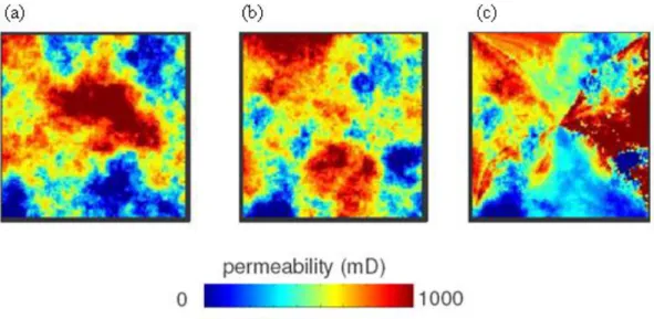
Figure 1.4: (a) 4D-seismic-saturation anomaly in a „black and white‟ format; (b) calculated reservoir permeability using 4D seismic; and (c) true reservoir permeability (Landa and Horne, 1997). ... 14

Figure 1.5: Fluid-front history-matching to estimate permeability (Kretz et al., 2004). ... 14

Figure 1.6: Five-spot synthetic case in which the fluid front has been matched: (a)–(c): reference, initial and updated permeability fields (Kretz et al., 2004) ... 15

Figure 1.7: (a) Actual permeability field; (b) inverted permeability field from true underlying pressure field; (c) inverted permeability field using a homogeneous pressure field; and (d) inverted permeability field using an iterated homogeneous pressure field. ... 17

Figure 1.8: (a) The reference permeability model; (b) the final permeability model; and (c) amplitude changes between 180 and 670 days (after Vasco et al., 2004). ... 20

Figure 1.9: (a) Reference permeability model; and (b) recovered permeability model (after Vasco, 2004). ... 20

Figure 1.10: Synthetic test: (a) reference permeability, and (b) the recovered permeability map (after MacBeth and Al-Maskeri, 2006). ... 21

(15)

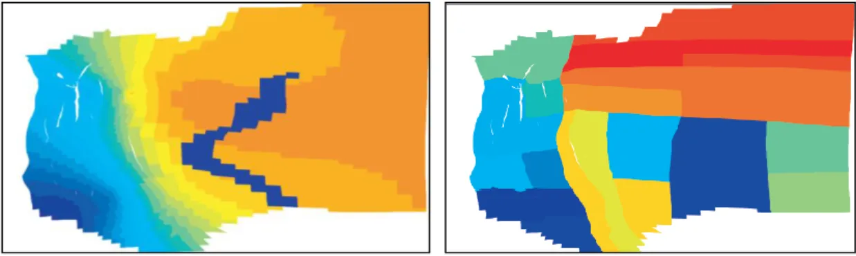
Figure 1.11: Field Application of the technique proposed by MacBeth and Al-Maskeri (2006): (a) vertically averaged permeability from the existing simulation model, and (b) resolved permeability for the same section of the field. ... 21

Figure 1.12: Qualitative interpretation for updating a reservoir flow simulation. ... 23

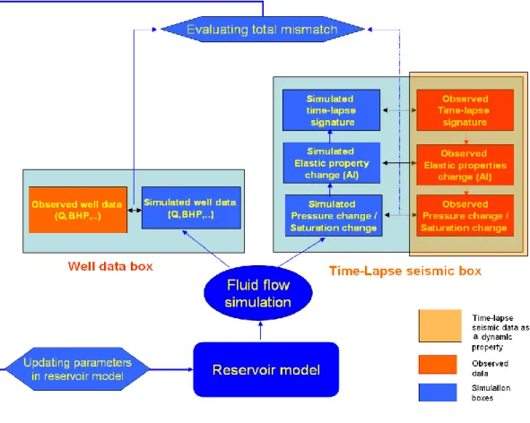
Figure 1.13: General workflow of the seismic history-matching workflow and data-match possibilities ... 24

Figure 1.14: Update of the simulation model, using 4D seismic as a reservoir-property estimator. ... 25

Figure 2.1: The saturation front arrives after the pressure profile is established. ... 28

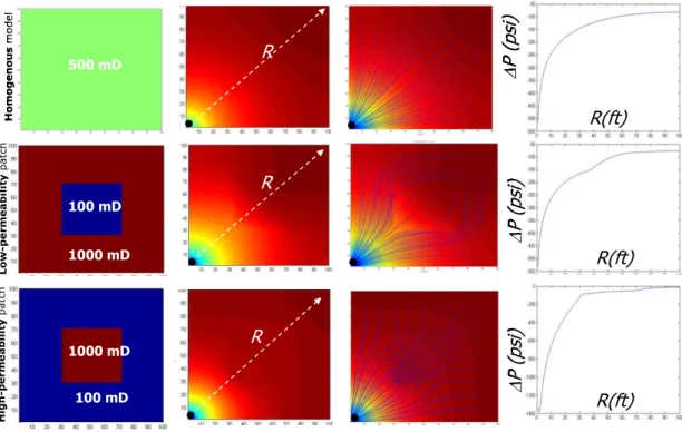
Figure 2.2: The effect of permeability on the pressure-change response: (a) synthetic cases for high-permeability, low-permeability and the homogeneous model, and (b) the time-lapse change in pressure for each of the permeability cases; (c) the streamlines of flow; and (d) the identification of the permeability signature of the time-lapse pressure change in the cross-sectional profile along the diagonal of the model (R). ... 31

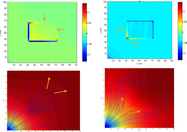
Figure 2.3: Calculated Laplacian and streamlines demonstrating the gradient fields for the case of (a) high-permeability patches; and (b) low-permeability patches... 33

Figure 2.4: Absolute value of the calculated Laplacian for the pressure response of the high-permeability patch model, using (a) the numerical central difference; (b) the Laplacian of the Gaussian; (c) the polynomial; and (d) the divergence of the gradient. ... 34

Figure 2.5: The pressure change, gradient and Laplacian of pressure change are computed for various permeability models. The bottom row shows the horizontal cross-sectional profile of pressure change in row 30, the Laplacian, and the absolute value of the Laplacian. ... 35

Figure 2.6: Permeability signature identification using the Seis2perm and recovering the permeability from pressure-change data, using the Laplacian... 37

(16)

Figure 2.8: High Laplacian magnitudes at the edges of the permeability region are a direct effect of the sudden change in pressure. This change grows in the gradient terms, and then in the Laplacian calculation. ... 40

Figure 2.9: (a) Time-lapse signature between 1993 and 1999 in the Schiehallion field; (b) the Laplacian of pressure-dominated time-lapse amplitudes; and (c) the absolute value of the Laplacian indicates edge problems in a field application: i.e. due to dominating edge effects, a high Laplacian is observed where a high-permeability region is expected based on the other available permeability data in the field. ... 40

Figure 2.10: The smoothing on the calculated Laplacian needs to be applied in order to control and smooth the edge values. The black curve was originally calculated for the Laplacian of a high-permeability blocky model; the red curve is a Gaussian loss-pass filter applied to the Laplacian; and the blue curve is a moving average for a window defined around the boundaries applied to the Laplacian at the edges. ... 41

Figure 2.11: Pressure change after (a) 100 days after production; (b) 200 days after production; (c) 400 days after production; and (d) 700 days after production. Due to pressure diffusion, the pressure disturbance is moving with time. ... 42

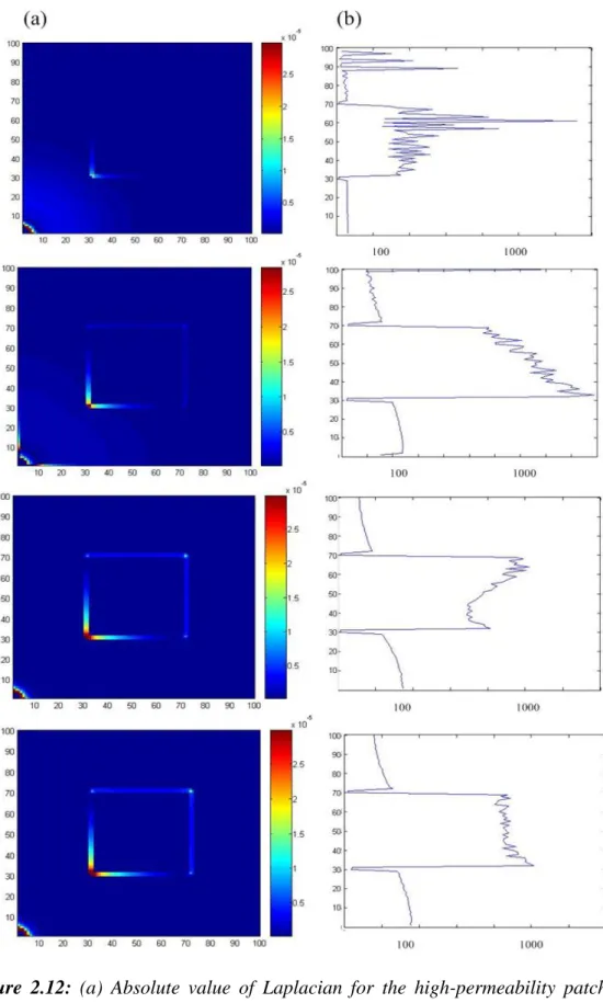
Figure 2.12: (a) Absolute value of Laplacian for a high-permeability patch model after 100, 200, 300 and 700 days‟ production (top to bottom), and (b) cross-section of the corresponding calculated permeabilities at cell 50. ... 43

Figure 2.13: (a) Time-lapse seismic signatures between 1993 and 1999, and (b) calculated Laplacian. ... 45

Figure 2.14: Estimated porosity from the 1993 base-line seismic. ... 46

Figure 2.15: Validation of linear approximation of pressure variation in this reservoir: the red curves correspond with a cell between two injectors but away from most of the producers, whilst the black curves correspond with a cell in the vicinity of a producer (after MacBeth and Al-Maskeri, 2006). ... 48

(17)

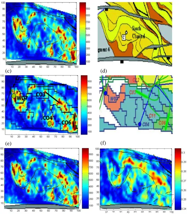
Figure 2.17: (a) and (b) A comparison of the estimated permeability pathways with the Schiehallion facies map (after Leach et al., 1999) shows a fair agreement between the calculated permeability pathways and the major and minor channels of the T31a sand; (c) and (d) show that the sparse pattern of permeability is consistent with Schiehallion compartmentalization (after Dobbyn and Marsh, 2001); and (e) and (f) comparison of the estimated permeability with the effective porosity shows correlation through the channel orientations. ... 50

Figure 2.18: The Seis2perm transform is applied to the southern part of the Girassol field. Comparing the estimated permeability with the simulation model, the solution appears to be in fair overall agreement with the depth-averaged permeability, although the locations of the main highs and lows are somewhat different. ... 52

Figure 2.19: A Seis2perm transform is applied to pressure changes in the central part of the Girassol field. The outline structure of the permeability is very similar to the simulation model. ... 53

Figure 3.1: Workflow of the direct updating of the simulation model, using 4D seismic-produced permeability. ... 58

Figure 3.2: Resampling of the seismic property to the reservoir-simulation grid. ... 59

Figure 3.3: Rescaling cell values to match the column average. ... 61

Figure 3.4: (a) Average permeability from the simulation model, and (b) multipliers values. In this section, there are four active wells in the time period of this particular 4D seismic (1999–1993): two injection wells (C11 and C12), and two horizontal production wells (P3 and P4). ... 63

Figure 3.5: (a) Simulation permeability model prior to integrating the 4D-seismic permeability, and (b) the updated simulation permeability model after including the 4D seismic permeability using the Seis2perm scheme. ... 64

Figure 3.6: Comparison of models after the history-matching process: (a) initiated from the operator model, and (b) initiated from the model with integrated 4D-seismic permeability... 68

(18)

Figure 3.7: (a) Water-cut in the production well P1, and (b) in a group of production wells (P1 and P2), after history matching (HM) the base case and the 4D–seismic-updated model. ... 69

Figure 3.8: (a) Comparison of the fit between observed total-field gas production, and the simulated one in different models, and (b) comparison of the fit between observed bottom-hole pressure for well P1 and the simulated one in different models. ... 70

Figure 3.9: Schematic of history matching using 4D seismic (Stephen and MacBeth, 2006) ... 74

Figure 4.1: The shape of the data is preserved by applying statistical normalization from (a) the 1996 RMS attribute, to (b) the normalized 1996 RMS attribute, with the mean equal to zero and the standard deviation equal to one. ... 82

Figure 4.2: Various attributes for the 1999–1993 and 2000–1993 time-lapse surveys. 83

Figure 4.3: Various attributes for 2002–1996 and 2004–1996 time-lapse surveys. ... 84

Figure 4.4: Uncertainty analysis for time-lapse surveys and attributes: (a) mean value of differrent attributes. (b) standard deviation of different attributes, (c) mean value of different 4D-seismic surveys, and (d) standard deviation of different 4D-seismic surveys. ... 85

Figure 4.5: (a) Correlation between the attributes, and (b) correlation between a specific attribute at different times. The correlation is higher between different attributes, due to the high production activity over aq reservoir‟s lifetime. ... 86

Figure 4.6: (a) Summation of the data for each bin, over all of the maps, and (b) standard deviation of the data for each bin, over all of the mapped 4D signatures. ... 89

Figure 4.7: (a) The mean of normalized data for each bin, over all of the maps, and (b) the standard deviation of the data for each bin, over all the mapped 4D signatures. .... 89

Figure 4.8: (a) NTG calculated from the coloured inversion base-line seismic (1996 seismic data using a model adapted from Connolly‟s method; (b) NTG from the

(19)

simulation model; and (c) NTG estimated from the base-line seismic attribute without removing the tuning effect. ... 92

Figure 4.9: Map of the standard deviations, indicating the spatial uncertainty of the seismic net-to-gross estimates. ... 92

Figure 4.10: (a) Multi-4D attributes response; (b) pressure change between 1998 and 2004 from the simulation model; (c) water-saturation change between 1998 and 2004 modelled from the simulation model; and (d) gas-saturation change between 1998 and 2004 modelled from the simulation model. ... 95

Figure 4.11: Recovering permeability for the synthetic blocky model with 1000 mD permeability; two scenarios are considered: the production-depletion and the production–injection pair for water-flooding. The Cp and Cs terms in the Floricich et al. technique (2005) are used to weight the pressure/saturation impact on the 4D seismic signature and to predict the consequence of pressure assumptions in the Seis2perm technique for recovering permeability. ... 97

Figure 4.12: The permeability is up-scaled between corresponding horizons to the top and base of reservoir T31a in the Schiehallion field. The map shows the up-scaled permeability values at well locations. These values are used for the calibration of the 4D-seismic-estimated permeability. ... 99

Figure 4.13: Connectivity assessment procedure by Shams et al. (2007) applied to the Girassol field, located in the Gulf of Guinea, Angola... 101

Figure 4.14: Permeability estimation in the Marlim field, Brazil: (a) 4D difference map for 2005–1997, where light blue indicates heavy oil replaced by water; (b) introducing a 4D anisotropy map into permeability by kriging with external drift; and (c) permeability of a simulation model after the history-matching process (after Oliveira et al., 2007). ... 102

Figure 4.15: (a) Standard deviation for the resulting permeability; (b) the enhanced estimated permeability; and (c) the vertically averaged permeability from the simulation model. ... 104

(20)

Figure 4.16: Mean permeabilities derived from different attributes, compared with reservoir simulation permeability using cross-sections in the x- and y-directions. The calculated error for the estimated permeabilities is specified. ... 105

Figure 5.1: (a) Global connectivity between wells (after Gentil, 2005), and (b) local connectivity from cell to cell ... 109

Figure 5.2: How connectivity terms used in the study are fitted and related to each other. ... 111

Figure 5.3: The hydraulic sand connectivity is calculated in the α product. The α product is a useful estimate in which channel presence is boosted and 4D-related noise is filtered (after Shams et al., 2007). ... 113

Figure 5.4: (a) Porosity; (b) permeability; and (c) NTG for models used to compute synthetic time-lapse saturation and pressure changes. Three water injectors are indicated by open circles, and two producing wells are denoted by black circles. ... 117

Figure 5.5: impedance versus NTG and permeability in forward modelling. The P-impedance appeared to be a direct function of NTG and the weaker function of permeability... 119

Figure 5.6: (a) Transmissibility is a mixture effect of the permeability and NTG- see Figure 5.4 (b) and Figure 5.4(c) respectively, (b) P-impedance, is affected substantially by NTG.. ... 120

Figure 5.7: (a) NTG; (b) saturation profile after 365 days‟ production; and (c) the pressure profile simulated after 365 days‟ production. ... 121

Figure 5.9: (a) Relative water permeability as a function of water saturation, Krw; (b) relative oil permeability as a function of oil saturation, Kro; (c) oil viscosity (cP) as a function of pressure. (Note that water viscosity is considered to be a constant value of 0.50 cP); (d) total mobility distributions within the reservoir after 365 days of

(21)

(however, the impact of saturation is substantial here); and (e) the modelled time-lapse change in acoustic impedance. ... 123

Figure 5.10: Darcy-derived connectivity in the sequence of survey times: (a) 1999– 1998; (b) 2000–1999; (c) 2001–2000; (d) 2002–2001; (e) 2003–2002; and (f) the sum of all difference maps, which is equal to total reservoir connectivity. ... 124

Figure 5.12: (a) Total reservoir connectivity calculated from Darcy-derived coonectivities; (b) the seismic-connectivity attribute calculated from hydraulic sand connectivities; and (c) the seismic-connectivity attribute (SCA) is proportional to the total reservoir connectivity. ... 127

Figure 5.13: Effect of compartmentalization on the pressure profile: (a) profile of the compartments; (b) transmissibility of the model; (c) and (d) pressure- and saturation-changes from the simulation between 1998 and 1999; (e) and (f) pressure- and change between 1999 and 2000; and (g) and (h) pressure- and saturation-changes between 1998 and 2000... 130

Figure 5.15: (a) NTG; (b) compartments; (c) the saturation profile on April 2004; and (d) pressure profile in April 2004 in segment 1 of the Schiehallion field data. ... 132

Figure 5.16: Forward and inverse routes, indicating how transmissibility and transmissibility multipliers are linked to the 4D-seismic response. ... 133

Figure 6.1: A general workflow in this chapter for transmissibility and transmissibility-multipliers estimation in the Schiehallion field. ... 138

Figure 6.2: NTG calculated using the Connolly method (2007). Note that the tuning effect is removed by using this method to underline the true response of the channels.

(22)

Figure 6.3: The coherency attribute identifies potential barriers to flow and channel margins. The nature of the boundaries identified by the coherency attribute is likely to be the result of a lithology contrast caused by faulting, facies change, or both. ... 141

Figure 6.4: (a) and (b) Laplacian features (type-P and type-S) and an illustration of how they are related to pressure- and saturation-anomalies; and (c) corresponding features observed in 4D seismic, indicating saturation (type-S) and pressure (type-P) anomalies. ... 143

Figure 6.5: A 2004–1996 RMS difference map extracted with a window defined from 10 ms below the top horizon to 40 ms above it. The difference map shows the movement of water from injectors to producers. Note that hardening around the injectors is indicated in blue, and softening is in red. The hardening effects around the injectors are correlated with high-NTG regions calculated from 3D seismic, indicating that the 4D anomaly is related to saturation change. However, softening around CW16 is due to pressure-up in the compartment, as the presence of a sealing fault is confirmed by comparing the coherency map from 3D seismic with the change in 4D seismic polarity across the fault. ... 145

Figure 6.6: The longest time taken for pressure to reach the boundary of this triangular compartment is 12 days for average properties of Schiehallion (The modelling is performed using Pansystem software). ... 147

Figure 6.7: (a) Identification of a pressure anomaly from the saturation around well CW13. The shape of the pressure anomaly is preserved between survey 04-96 and 08.04, whereas the saturation anomaly has evolved from survey 04-99 to survey 06-04, and (b) identification of a pressure compartment around injection well CW16 and production well CP05_C05. Again the shape of the pressure anomaly is preserved between surveys 04-02 and 04-96. A water-saturation anomaly around CW16, and a gas-saturation anomaly around CP05, are also observed. ... 148

Figure 6.8: (a) Summation of saturation anomalies from different surveys. The anomalies around the injection wells (in blue) are indicating hardening due to water injection, while the anomaly around the production well (for example, CP23_B is

(23)

saturation differences calculated and summed together as predicted from the simulation model. ... 150

Figure 6.9: (a) Compartmentalization evaluated from the pressure-anomaly map, and (b) compartmentalization in the simulation model. ... 151

Figure 6.10: The field is subdivided into regions, using the determined pressure-anomaly map. Transmissibility multipliers for the zone of pressure communication between the polygons obtained is calculated using well-production data. The transmissibility multiplier can represent a barrier without using a cell. ... 152

Figure 6.11: (a) The BHP of injection well CW16 versus production well CP05; (b) the BHP of injection well CW16 versus production well CP06; and (c) the BHP of injection well CW17 versus production well CP06. Consistent behaviour in receiving the pressure impulses in a production well from an injection well implies a good communication. Data are averaged for every 30 days for visualization purposes. ... 154

Figure 6.12: The correlation coefficient measures the degree of linear dependence between two injection and production BHP variations. ... 155

Figure 6.13: A general workflow for estimating the transmissibility guided by the SCA map. The connectivity attribute is interrelated with transmissibility values which are defined to be average permeabilities at the interfaces between two grid blocks in the reservoir-simulation model. A non-linear relationship is assigned between these two properties. The conditional probability is calculated to incorporate the non-linear relationship and the uncertainty attached to this relationship. The assigned probability is then applied in a sequential Gaussian simulation framework to generate equi-probable realizations. ... 157

Figure 6.14: Calculated SCA in segment 1 of the Schiehallion field. ... 158

Figure 6.15: Relationship between the calculated connectivity and up-scaled transmissibility values at well locations. ... 160

(24)

Figure 6.17: Simulation transmissibility that is vertically averaged over the T31a reservoir. ... 162

Figure 6.18: Transmissibility is a function of permeability and NTG in a forward model calculation. For different NTG (sand facies), transmissibility is correlated to permeability with a different relationship. ... 163

Figure 7.1: Time-lapse attribute in the Nelson field for 2000–1990 surveys averaged from the top to the base horizon. Green to red indicates water movement, while blue indicates no change (after Stephen et al., 2007). ... 171

Figure 7.2: There are three ways in which 4D seismic can be used to update the reservoir model: updating the facies; updating the petrophysical properties in the geological model; and updating the reservoir properties in the simulation model. ... 174

Figure 7.3: Combining the FTHM and SHM methods will reduce the non-uniqueness in seismic-history inversion, and can quickly provide a reduced misfit between the observed and predicted data ... 175

Figure 7.4: A maturity S-curve for different 4D applications (after Staples et al., 2006). ... 179

Figure A.1: The 2D x/y grid, showing the control volume. ... 181

Figure E.1: (a) A wedge model consisting of a wavelet convolved with a thickening boxcar impedance profile showing the tuning effect, and (b) the apparent time thickness is the time separation between the top and base reservoir horizons picked along zero-crossings of coloured inversion seismic data (after Connolly, 2007). ... 191

Figure E.2: Seismic section through the pre-production 1996 base-line volume in the Schiehallion field: band-limited impedance obtained using coloured inversion. The T31a reservoir unit has been picked on the zero-crossingsof the top and bases. ... 191

Figure E.3: (a) Average RMS attribute extracted between the top and the base of the T31a reservoir, from 1996 pre-production base-line seismic, and (b) time thickness calculated between the top and the base of the reservoir. ... 192

(25)

Figure E.4: Successive stages of the detuning process: (a) the extracted wavelet for the data; and (b) the cross-plot of the average RMS attribute, plotted against the apparent thickness for the T31a reservoir unit – superimposed is a modelled tuning curve; (c) modelled seismic net-to-gross; and (d) detuning correction curve. ... 193

Figure E.5: Frequency spectrum for the wavelet extracted for the T31a reservoir. Based on the estimated wavelet, a trapezoidal filter 5-10-50-60 is designed to simulate the wedge and therefore model the tuning response. ... 194

Figure F.1: Discretization and notation for the 2D equation ... 198

Figure I.1: Cumulative water injection at well CW13, and (b) BHP (blue represents the daily BHP fluctuations, and red represents the moving average over a period of a month) at well CW13. Comparison with the well data identifies the fact that the signal in the 4D seismic is affected by pressure or saturation. ... 209

Figure I.2: (a) Petro-elastic model (after Marsh, 2004); (b) saturation change between 1998 and 1999, from the simulation model; (c) pressure change between 1998 and 1999, from the simulation model; and (d) a time-lapse difference map between pre-production 1996 and 1999, interpretable based on the petro-elastic model and consistent with the pressure-saturation predictions of this simulation. ... 212

Figure I.3: (a) Saturation change between 1998 and 2004, from the simulation model; (b) the pressure change between 1998 and 2004, from the simulation model; (c) the observed 4D seismic between 1996 and 2004; and (d) the synthetic 4D response between 1996 and 2004 (Amini, 2009).. ... 213

Figure J.1: The likelihood function, which is calculated by extracting the 1D likelihood function from the joint PDF ... 214

Figure J.2: Local posterior probability calculation... 215

Figure J.3: Sequential Gaussian simulation with seismic connectivity attribute conditional probability (adapted from Doyen, 2007). ... 216

(26)

CHAPTER 1: INTRODUCTION

1. INTRODUCTION

Overview

This chapter provides an introductory description of the various geophysical and engineering tools used for permeability estimation, and their advantages and disadvantages, and identifies the need for a time-lapse seismic method in permeability estimation. First, the various possible permeability-inversion approaches are described. Next, the use of permeability estimates in updating the reservoir simulation model is discussed. Finally, the main contributions of this thesis are addressed.

(27)

1.1 Introduction

New high-resolution time-lapse seismic data have led to the delivery of accurate quantitative interpretations. This has satisfied many reservoir-engineering objectives in reservoir management and monitoring. Time-lapse seismic interpretations have successfully contributed to the attainment of maximum hydrocarbon recovery at a minimum cost. The key concept in achieving maximum recovery is the role of time-lapse seismic in the development of the science of reservoir characterization.

Reservoir characterization involves building a reservoir model that incorporates the characteristics of the reservoir that are pertinent to storing and producing hydrocarbons. In reservoir characterization, a two-fold problem is considered: (1) the distribution of hydrocarbons through the reservoir, and (2) the likely fluid pathways towards the producing wells.

The reservoir model must provide a description of the reservoir that correctly accounts for the spatial variation and continuity of the porosity, permeability and fluid saturation that are essential for storing hydrocarbons and transforming hydrocarbons. The reservoir property that provides the necessary pathways for hydrocarbon flow towards the production wells is permeability. In reservoir characterization, after the Initial Oil In Place (IOIP) and aquifer properties, it is important to determine the permeability. An accurate estimate of permeability is crucial, because, in most fields, it is the most important parameter that affects the reservoir performance (Yoon et al., 1999). It controls the behaviour of the simulation model designed as the basis for well-completion strategies, production, and reservoir management. Most of the sensitivity analysis prior to history matching in reservoir simulation has shown that, generally, permeability values, fault multipliers, and transmissibilities are among the parameters to be adjusted for achieving an optimal match in the reservoir-simulation model (Harpole and Hearn, 1982). For example, Jian et al. (2004) built 50 reservoir models, varying the combinations of parameters using experimental design technique. They ran the simulation for these models, and they showed that there are large differences (some greater than 200%) in water-cut, breakthrough time, water production and oil recovery. These differences in the model predictions were found to be due to changes in the horizontal permeability between the models.

(28)

The accuracy of reservoir management and strategies for future prediction of the reservoir are tied to the accurate and reliable permeability measurements based initially on the simulation model. Despite the crucial importance of accurate permeability estimation, the generation of permeability models that best describe the reservoir heterogeneity sometimes seems to be a difficult target to achieve. The conventional capabilities of permeability estimation, such as well logging, cores and well testing, suffer from unreliability beyond the wells, because their evaluation is limited to the borehole region. Permeability estimation between the wells is vital in constraining the reservoir model. Hence, there is a critical need for a new technology that can provide this type of information.

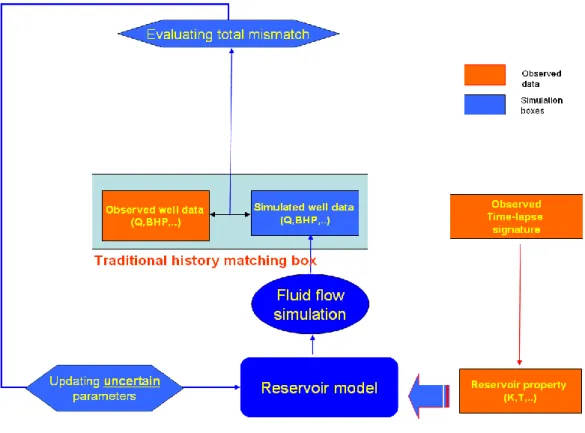
Recently, the number of new techniques of delivering high-resolution dynamic information using time-lapse seismic has increased. This has led the industry to examine the practice of evaluation of reservoir properties, such as the location of sealing faults, flow barriers or high-permeability pathways, and general field-wide pressure- and saturation-changes (MacBeth et al., 2005). Now an important question in a reservoir-engineering context is: how far can time-lapse seismic go in the refinement of the reservoir-simulation model. Based on this philosophy, current work has concentrated on efforts to establish a new role for time-lapse seismic in the prediction of the most challenging reservoir property: permeability. In fact, it would be an outstanding achievement for time-lapse seismic to extract permeability across the field with a reasonable resolution. Further, to fulfil such an intention, an algorithm has to be designed to update the simulation model using the predicted results from the 4D seismic. The overall aim is to validate whether the 4D permeability product brings value to the history-matching process. The procedure proposed by the latter step addresses several challenging issues in simulation updating using seismic-scale products. Figure 1.1 is an illustration of the general workflow that gives an overview of the framework of the present work.

(29)

Prediction

Permeability estimator technique from 4D

Simulation

Tackling scaling issue

Well data Calibration

Estimated mapped values of K

4D attributes

Seis2perm method Permeability estimation from 4D seismic

Updating the reservoir flow-simulation

Evaluating the value of 4D seismic permeability product in history matching

General workflow steps:

1. Permeability estimation from 4D seismic 2. Tackling scaling issues

3. Updating the reservoir flow-simulation 4. History matching 3D volumetric values of K in reservoir model Prediction Prediction Permeability estimator technique from 4D Simulation

Tackling scaling issue

Well data Calibration

Estimated mapped values of K

4D attributes

Seis2perm method Permeability estimation from 4D seismic

Updating the reservoir flow-simulation

Evaluating the value of 4D seismic permeability product in history matching

General workflow steps:

1. Permeability estimation from 4D seismic 2. Tackling scaling issues

3. Updating the reservoir flow-simulation 4. History matching

3D volumetric values of K in reservoir model

Figure 1.1: 4D-seismic-derived horizontal permeability is used to update the simulation model.

1.2 Permeability measurement

Although permeability is an important rock property (Ahmed et al., 1989), it is one of the most difficult of all petrophysical properties to determine (Johnson, 1994). The conventional sources for permeability determination provide a formation permeability that represents different averaging volumes. Core analysis, well-test analysis and well logs are conventional tools used to measure the permeability. 3D seismic is also a new potential tool introduced to infer permeability. However, it is still highly controversial and not yet entirely proven as described in section 1.2.5. The following section gives a brief review of the range of permeability-estimation methods, describing how they measure the permeability and listing the shortcomings attached to their measurement.

(30)

1.2.1 Core-determined permeability

Permeability is usually determined from core analysis. Permeability determination using core analysis is considered as a standard measurement such that the permeability derived from all other methods is usually compared with the core permeability. The procedure to establish the permeability starts with cutting core plugs from the whole core, and then cleaning and drying the core plugs; then flow is induced at several rates. For each flow rate, the inlet and outlet pressures are measured. Finally, the permeability is calculated using the slope of the graph in which the flow rate is plotted versus the pressure function across the faces of the sample.

Conventionally, core permeability is then populated through the geological facies, using geostatistical methods, and this is utilized as the initial permeability model for future flow-simulations. The procedure involves establishing a relationship between plug permeability, porosity and facies. The facies in the reservoir volume are delineated by conditioning to 3D seismic and wireline logs. Once porosity is assigned using the facies model, the permeability can be established, based on the porosity–permeability relationship derived from core plugs.

Although the practice of measuring the permeability using cores provides high resolution estimation, in reality high-quality core-based permeability data are difficult to achieve, either because of the borehole conditions or due to the high cost of coring. For these reasons, over the years attempts have been made to estimate permeability using alternative methods. One of the comparatively inexpensive and readily available sources of inferring permeability is well-logging information.

1.2.2 Using wireline logs to determine permeability

Various models have been used to estimate permeability using correlations from well logs (Wyllie and Rose, 1950; Timur, 1969; Coates and Dumanoir, 1974). Most of these correlations are established directly from core-plugs, attempting to relate a commonly logged property such as porosity (φ) and/or Vclay to permeability (K). These correlations

are generally semi-log in nature (such as φ = aLn(K) + b). The second type of correlation incorporates information from water saturation estimated from resistivity

(31)

logs combined with Archie‟s equation (1949). For example, Wyllie and Rose (1950) proposed the following equation for determining permeability:

                  w 1 2 2 c 1 S F P A K m (1.1)

where F is the resistivity factor; Sw is connate water saturation; Pc is capillary pressure; A is a constant value, which varies for different lithologies; and m is the cementation factor. Recently, NMR (nuclear magnetic resonance) log technology has been used in inferring permeability. This is a relatively new technique (Coates et al., 1999). NMR uses hydrogen protons as an indicator of the presence of fluids in the pore space of porous media.

All methods of permeability determination from well logs use an indirect relationship via various physical properties of the rock and fluid. The relationship is not often well defined. Moreover, the correlations of permeability with porosity and water saturation are limited because the portions of the porous medium that dominate permeability, porosity and water saturation are different (see Figure 1.2). Permeability is dominated by the pore throats, while porosity and water saturation are dominated by the volume within the pore bodies. Hence, correlations for permeability are inherently limited when correlating to porosity and water saturation or any other rock property that is strongly influenced by any part of the porous media other than the pore throat. Even in NMR technology, as Kenyon (1997) points out, while the objective is to measure the throat size (the dominant effect on permeability), the NMR logs provide information about pore size. Although they are related to each other, this may not be very realistic in a quantitative model as expressed in Kenyon‟s equations. In conclusion, there is no direct method to determine permeability using well logs.

(32)

Figure 1.2: Schematic picture defining a throat and a pore in the pore space of a porous material. Permeability is related to the throat size of a porous medium, whereas porosity and saturation are related to pore-size distribution.

1.2.3 Well-test permeability estimation

The calculation of the so-called effective well-test-derived permeability is based on the interpretation of a pressure-transient well test. Usually, such a well test consists of generating some flow-rate impulses in the reservoir by build-up and drawdown and then observing the resultant pressure response. A number of techniques are available to perform pressure-transient analysis (Sabet, 1991). Generally, in most of these techniques, the following diffusivity equation is solved:

t P K c r P r r P         _t 2 2 1  (1.2)

where P(r,t) is pressure, r is the radial distance from the well-bore, t is time, φ is the porosity, μ is the viscosity, ct is the total compressibility, and K is the absolute

permeability. The use of Equation 1.2 implies the following assumptions: (1) flow is radial; (2) the well is open over the entire vertical thickness of the reservoir; (3) the reservoir is homogeneous and isotropic; (4) the fluid has constant properties and slight compressibility; and (5) the pressure gradients are small and gravitational forces are negligible. For the transient period (the period in which the pressure disturbance has not reached the boundary of reservoir), the following boundary and initial conditions apply:

0 , ) , ( , ) 0 , ( i i         r__ r P P t r P P t r P (1.3)

(33)

                Kt r c E Kh qB P t r P t 4 2 1 2 ) , ( 2 i i    (1.4)

where P(r,t) is the pressure at a given radius r and time t; Pi is the initial reservoir

pressure; h is the reservoir thickness; q is flow rate; B is the formation volume factor; K is absolute permeability; and Ei is the exponential integral function that is defined as:

u u x E x u d e ) (



     (1.5)

For all but very early times, the Ei function can be approximated by a logarithmic

function, and Equation 1.4 can be rewritten as:       _   ln 0.80907 4 ) , ( i ₂ cr Kt kh qB P t r P    (1.6)

Using Equation 1.6, a semi-log plot of pressure versus time should produce a straight line for the early linear response, from which the effective well-test permeability can be determined by this equation:

mh qB

K 162.6  (1.7)

where m is the slope of the semi-log straight line. The permeability K represents an effective average of the absolute permeability within the reservoir volume drained by the well test. In fact, the solution of the diffusivity equation (Equation 1.2) is based on the assumption that the reservoir is homogeneous; however, no reservoir is homogeneous, and the degree of heterogeneity is a function of the lithology, depositional and post-depositional environment of the reservoir. For practical purposes, it is assumed that the permeability determined by well-test analysis is an effective permeability representing some average within a radius of investigation or drainage radius, which is influenced by the producing well. In other words, the well-test result is insensitive to small-scale heterogeneities. Grader and Horne (1988) showed that it is possible to have a sizeable „hole‟ in the reservoir without making any discernible difference to an interference test. The definition of radius of drainage is questionable in the presence of heterogeneities (Matthews and Russell, 1967). Many attempts have been

(34)

made to estimate the effective response of the heterogeneous model without recourse to numerical simulation (Beggs and King, 1985; King, 1989; Duquerroix et al., 1993; Vega, 1995). However, no analytical solution has been found that accounts for all parameters affecting fluid flow. To overcome the limitations of conventional well test that is indicative of near wellbore homogenous permeability, the well interference test is introduced as an alternative that provides regional permeability trend and conveys permeability anisotropy. The well interference test involves a cyclic injection of fluid into the source well (that is associated with changes in rates), and measurement of the pressure pulse in a neighbouring well (known as observation well). Type curves are utilized for interpreting pulse interference tests and provide detailed hydraulic characterization including permeability evaluation between wells. Although this technique is usually have more precision than conventional well testing methods, it usually takes considerable time for production at one well to measurably affect the pressure at an adjacent well. Consequently, interference testing is more expensive and there is a difficulty in maintaining fixed flow rates over an extended time period (Dyer, 2007).

1.2.4 History matching for updating permeability

Generally, it is possible to improve the permeability field in the history-matching process (Fasanino and Molinard, 1986; Ouenes, 1992; Grimstad et al., 2004). In this process, the production data are used to infer permeability/transmissibility values so that the model prediction matches the observed data. For example, Fasanino and Molinard (1986) defined an objective function based on a measured pressure distribution. The transmissibility values are iteratively modified until the gradient descends to the smallest value of the objective function. Ouenes (1992) also presented an automatic history-matching algorithm that simultaneously estimates relative permeability and capillary pressures for core floods using the optimization method of simulated annealing. Grimstad et al. (2004) also showed how unknown large-scale permeability structures such as channels or barriers can be identified by history matching, using adaptive multi-scale estimation (AME) (Figure 1.3). They assumed that the true permeability field is known. Then they used this reference permeability in a „field-scale synthetic model‟ to generate bottom-hole pressures and fluid well rates. These production data were then used as the information for the permeability identification.

(35)

a) b)

Figure 1.3: History matching for estimation of permeability: a) Reference permeability,

b) Final permeability result using AME. Grimstad et al. (2004)

(a) (b)

Figure 1.3: History matching for estimation of permeability: (a) reference permeability, and (b) final permeability result using AME (after Grimstad et al., 2004).

The studies mentioned show the promise of using optimization techniques to estimate reservoir properties. However, such applications are computationally expensive and time-consuming. Moreover, they can provide no more than the general trend or large-scale variation of the property. The final resolution of an optimized model depends on the cell size, and usually produces a very coarse-scale view of the permeability field.

1.2.5 Using 3D seismic for permeability estimation

One of the first attempts to address the problem of estimating permeability from seismic data was done by Maurice Biot (1956). Biot recognized a frequency-dependent analytical relationship between permeability and seismic attenuation. However, laboratory, sonic log, cross-well, VSP (Vertical Seismic Profile), and surface seismic have all demonstrated that Biot‟s predictions often greatly underestimate the measured levels of attenuation. In 2001, the Department of Energy at Berkeley University brought together 15 participants from industry, national laboratories, and universities to concentrate on whether permeability can be determined from the seismic data (Pride et al., 2003). They investigated whether the permeability of the rock in which the seismic wave propagates influences the amplitudes versus distance. They considered attenuation mechanisms as a controlling issue to address this question. They concluded that there is a hope that the structure of permeability for a geological formation may be resolved at a specific degree of resolution. However, they found their calculation to be beyond the capabilities of the computers at that time, and they are hopeful that future technological developments and further research will be able to solve the problem. Other researchers,

(36)

same concept to infer permeability from 3D seismic. Klimentos and McCann (1990) used the relationship between attenuation and porosity, and then inferred the permeability map indirectly (if a core-based porosity–permeability relationship could be established). Shapiro and Müller (1999) investigated the link between permeability and attenuation for heterogeneous media. They noticed that in such structures, two effects are of importance for seismic attenuation: interlayer flow or the process of diffusion and elastic scattering of seismic waves. They showed that the frequency dependence of the P-wave attenuation coefficient and its anisotropy are sensitive to the permeability, especially at lower frequencies. They also concluded that the permeability that controls the seismic attenuation can differ very strongly from the hydraulic permeability. In summary, a survey of the literature shows that, as yet, investigations have shown that there is no clear and direct relationship between the 3D seismic signal and permeability.

1.3 Why estimate permeability from 4D seismic?

When considering conventional methods of permeability estimation, it seems that the requirements of the reservoir engineer cannot be fulfilled by the methodologies that are currently available. A brief overview of these methodologies is listed in Table 1.1, in which a comparison has been made between the various methods of permeability determination. Permeability data taken from cores have an excellent vertical resolution and no lateral resolution. Usually only a small percentage of the field is cored, which gives only a poor aerial coverage. Well-test permeability does not have the required vertical resolution, as it is an average for the interval from which the well is drained. However, it has a good lateral resolution (with a variable radius of influence). Although well-test information provides aerial coverage of the field, especially for well-developed reservoirs, the medium-scale formation heterogeneity cannot usually be resolved by conventional well-test data. Log-derived permeability data have both the required vertical resolution and a slightly better lateral resolution. But this is not a direct method of permeability measurement, as it is usually calculated through correlations with other properties. Moreover, its aerial coverage (lateral resolution) is limited to the areas close to the well-bore. Generally there are some inherent uncertainties in the above-mentioned methods. Furthermore, each of these methods is unreliable beyond a few sample locations of the well. The permeability evaluation in the regions away from the wells remains crucial in constraining the simulation model and predicting the accurate future

(37)

behaviour of the reservoir. An alternative tool is required to provide the permeability values between wells. The domain of seismic data is the only suitable source of information that provides spatial coverage over the entire field. As discussed, 3D-seismic data cannot be easily converted to permeability estimates. However, the permeability derived from time-lapse seismic is a promising tool that can enhance the permeability estimation in inter-well space. In fact, the new tool can fill the gap in conventional techniques in terms of lateral coverage, aerial resolution and also providing sufficient information on connective pathways and barriers.

Table 1.1: Comparison of the different tools used for the measurement of permeability

Timing Comments Aerial coverage Resolution Data Included in geological model High level of uncertainty on the inferred trends Poor – sparse in 1D Excellent vertical resolution (0.05–0.1 m) Cores Included during initial geological model Indirect conversion to permeability 1D

Very good vertical and horizontal (0.1–1 m) Wireline logs

WT: carried out over a few days or weeks. WIT: takes more time compared with conventional WT. WT: are done

throughout the life of the field in order to refine the estimates WIT: is expensive to run Extends partly into 2D – variable radius of influence WT: Poor vertical and

moderate horizontal (e.g. 30 m by 30 m by 10 m)

WIT: Good horizontal resolution between wells (depends on distance between wells) Well tests (conventional and Well Interference Test) Time-consuming task History-match resolution depends on the cell size and the flow regime Coarse 2D

scale, as based on well data Poor to moderate

vertical and horizontal (e.g. 100 m by 100 m by 3 m) History match on rates/water-cuts and pressures Static information only Use of attenuation, or porosity, still highly debatable Potentially excellent Good horizontal and

poor vertical (e.g. 12.5 m by 12.5 m by 12 m) 3D seismic

Over a few years, depending on the survey frequency Overall, has the

highest potential to deliver value Potentially

excellent Good horizontal and

poor vertical (e.g. 12.5 m by 12.5 m by 12 m) 4D seismic