Heterogeneous Sensor Signal Processing for Inference with Nonlinear Dependence

(1)

SURFACE

Dissertations - ALL SURFACE

December 2015

Heterogeneous Sensor Signal Processing for Inference with

Nonlinear Dependence

Hao He

Syracuse University

Follow this and additional works at: https://surface.syr.edu/etd

Part of the Engineering Commons

Recommended Citation Recommended Citation

He, Hao, "Heterogeneous Sensor Signal Processing for Inference with Nonlinear Dependence" (2015). Dissertations - ALL. 390.

https://surface.syr.edu/etd/390

This Dissertation is brought to you for free and open access by the SURFACE at SURFACE. It has been accepted for inclusion in Dissertations - ALL by an authorized administrator of SURFACE. For more information, please contact

(2)

Inferring events of interest by fusing data from multiple heterogeneous sources has been an interesting and important topic in recent years. Several issues related to inference using het-erogeneous data with complex and nonlinear dependence are investigated in this dissertation. We apply copula theory to characterize the dependence among heterogeneous data.

In centralized detection, where sensor observations are available at the fusion center (FC), we study copula-based fusion. We design detection algorithms based on sample-wise copula selection and mixture of copulas model in different scenarios of the true dependence. The proposed approaches are theoretically justified and perform well when applied to fuse acoustic and seismic sensor data for personnel detection. Besides traditional sensors, the access to the massive amount of social media data provides a unique opportunity for extracting information about unfolding events. We further study how sensor networks and social media complement each other in facilitating the data-to-decision making process. We propose a copula-based joint characterization of multiple dependent time series from sensors and social media. As a proof-of-concept, this model is applied to the fusion of Google Trends (GT) data and stock/flu data for prediction, where the stock/flu data serves as a surrogate for sensor data.

In energy constrained networks, local observations are compressed before they are trans-mitted to the FC. In these cases, conditional dependence and heterogeneity complicate the sys-tem design particularly. We consider the classification of discrete random signals in Wireless Sensor Networks (WSNs), where, for communication efficiency, only local decisions are trans-mitted. We derive the necessary conditions for the optimal decision rules at the sensors and the FC by introducing a “hidden" random variable. An iterative algorithm is designed to search for the optimal decision rules. Its convergence and asymptotical optimality are also proved.

(3)

tion Classification (AMC) problem. Censoring is another communication efficient strategy, in which sensors transmit only “informative" observations to the FC, and censor those deemed “uninformative". We design the detectors that take into account the spatial dependence among observations. Fusion rules for censored data are proposed with continuous and discrete local messages, respectively. Their computationally efficient counterparts based on the key idea of injecting controlled noise at the FC before fusion are also investigated.

In this thesis, with heterogeneous and dependent sensor observations, we consider not only inference in parallel frameworks but also the problem of collaborative inference where collab-oration exists among local sensors. Each sensor forms coalition with other sensors and shares information within the coalition, to maximize its inference performance. The collaboration strategy is investigated under a communication constraint. To characterize the influence of inter-sensor dependence on inference performance and thus collaboration strategy, we quantify the gain and loss in forming a coalition by introducing the copula-based definitions ofdiversity gainandredundancy loss for both estimation and detection problems. A coalition formation game is proposed for the distributed inference problem, through which the information con-tained in the inter-sensor dependence is fully explored and utilized for improved inference performance.

(4)

By

Hao He

B.S., Harbin Institute of Technology (HIT), China, 2010

DISSERTATION

Submitted in partial fulfillment of the requirements for the degree of Doctor of Philosophy in Electrical and Computer Engineering

Syracuse University December 2015

(5)

(6)

First and foremost, I would like to express my deepest gratitude and sincere thanks to my advisor, Prof. Pramod K. Varshney, for his guidance, support and encouragement during my doctoral study. I have been amazingly fortunate to have an advisor who gave me the freedom to explore on my own, and at the same time guidance to recover when my steps faltered. He has been influencing me with his enthusiasm towards research, as well as immense knowledge, and will keep guiding me in the future.

Besides my advisor, I would like to thank the rest of my thesis committee: Prof. Biao Chen, Prof. Lixin Shen, Prof. Qi Cheng, Prof. Mustafa Gursoy and Prof. Fritz Schlereth for their insightful comments and suggestions.

I would like to thank all my fellow labmates in the Sensor Fusion Laboratory for their constant support in my research and life: Yujiao Zheng, Swarnendu Kar, Sid Nadendla, Raghed Bardan, Nianxia Cao, Aditya Vempaty, Sijia Liu, Bhavya Kailkhura, Shan Zhang, Qunwei Li, Prashant Khanduri, Swatantra Kafle and Pranay Sharma. Es-pecially, discussions with Dr. Arun Subramanian and Dr. Satish Iyengar were very fruitful and triggered original ideas of part of this thesis.

Dr. Ruixin Niu guided me and encouraged me when I just started my program and some of his advice was beneficial throughout my entire doctoral study. Dr. Xiaojing Shen and Dr. Sora Choi have provided technical support for part of the work in this thesis.

My PhD research has been supported by US Army grants 09-1-0244, W911NF-14-1-0339 and W911-NF-13-2-0040 for which I am very grateful. The footstep data

(7)

like to thank Dr. Thyagaraju Damarla of ARL for providing very insightful sugges-tions on the research reported in this thesis

Most importantly, none of this would have been possible without the love and constant encouragement of my parents and my fiancee. I would like to thank them for always being there cheering me up and standing by me through the good times and bad.

(8)

Acknowledgments v

List of Tables xi

List of Figures xii

1 Introduction 1

1.1 Background . . . 2

1.1.1 Copula Theory . . . 2

1.1.2 Summary of Some Copula Functions . . . 4

1.1.3 Copulas and Measures of Dependence . . . 5

1.2 Literature Review . . . 6

1.2.1 Dependence as Covariance . . . 7

1.2.2 Nonlinear Dependence: Nonparametric Approach . . . 9

1.2.3 Nonlinear Dependence: Copula-based Approach . . . 10

1.3 Main Contributions and Organization . . . 11

1.4 Bibliographic Note . . . 14

2 Centralized detection under complex dependent observations 16 2.1 Motivation . . . 16

2.2 Problem Formulation . . . 17

2.3 Detection under Non-stationary Dependence . . . 21

(9)

2.3.2 Detection with Unknown Parameters . . . 25

2.3.3 Detection with Unknown Marginals and Unknown Copula Parameters . 26 2.4 Detection Using Mixture of Copulas . . . 28

2.5 Results and Discussion . . . 31

2.5.1 Nonstationary Copula . . . 31

2.5.2 Mixture of Copulas . . . 34

2.5.3 ARL Footstep Data . . . 37

2.6 Summary . . . 40

3 Copula-based Fusion of Heterogeneous Time Series 42 3.1 Motivation . . . 42

3.3 Copula-based Multivariate Dynamic Models . . . 46

3.3.1 Conditional Marginal Distributions . . . 46

3.3.2 Estimation and Inference for Copula Models . . . 48

3.4 Stock Prediction with Google Trends Data . . . 50

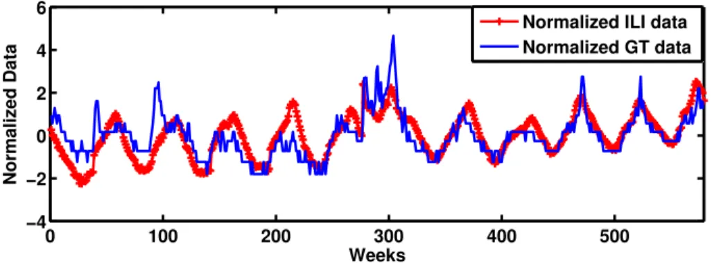
3.5 Flu Prediction with Google Trends Data . . . 54

3.6 Summary . . . 59

4 Distributed Classification under Dependent Observations 60 4.1 Motivation . . . 60

4.3 Design of Optimal Sensor Rules and Fusion Rule . . . 64

4.4 Computational Algorithm . . . 69

4.5 Example . . . 81

4.6 Summary . . . 83

(10)

5.3.1 Fusion of Analog Censored Data . . . 92

5.3.2 Fusion of Quantized-Censored Data . . . 95

5.4 Noise-aided Fusion of Analog Censored Data . . . 97

5.5 Noise-aided Fusion of Quantized-Censored Data . . . 99

5.5.1 A Review of Widrow’s Statistical Theorem of Quantization . . . 99

5.5.2 Computationally Efficient Fusion of Quantized-Censored Data . . . 101

5.6 Simulation Results . . . 106

5.7 Summary . . . 112

6 Coalitional Games for Distributed Inference in WSNs 114 6.1 Motivation . . . 114

6.1.1 Preliminary: Coalitional Game Theory . . . 117

6.2 System Model . . . 118

6.3 Collaborative Distributed Estimation . . . 120

6.4 Collaborative Distributed Detection . . . 128

6.5 Game Formulation and Properties . . . 135

6.5.1 Coalition Formation Algorithm . . . 137

6.6 Simulation Results . . . 139

6.7 Summary . . . 148

7 Summary and Future Directions 150 7.1 Summary . . . 150

7.2 Future Directions . . . 153

(11)

(12)

1.1 Archimedean copula functions . . . 5

2.1 Distribution of marginals for simulation experiments . . . 32

3.1 Behaviors of theoretical ACF and PACF . . . 47

3.2 MSE of different prediction approaches . . . 54

3.3 MSE of different prediction approaches . . . 58

(13)

2.1 ROCs forH1 data generated using atcopula . . . 33

2.2 ROCs forH1 data generated using Frank and Gaussian copulas . . . 34

2.3 ROCs forH1 data generated using a Frank copula . . . 35

2.4 Scatter plot: mixture of Gaussian (φ1 = 0.7, π1 = 0.5) and Gumbel (φ2 = 19, π2 = 0.5) . . . 36

2.5 Scatter plot: mixture of Gaussian (φ1 = 0.7, π1 = 0.5) and Gumbel (φ2 = 5, π2 = 0.5) . . . 36

2.6 Scatter plot: mixture of Gaussian (φ1 = 0.7, π1 = 0.5) and Gumbel (φ2 = 1.5, π2 = 0.5) . . . 37

2.7 ROCs forH1 data generated by the mixture of Gaussian and Gumbel. . . 38

2.8 Raw acoustic and seismic sensor data . . . 39

2.9 ROCs for the ARL dataset for 1 person vs. background detection. . . 40

3.1 The network of traditional sensors and social media. . . 44

3.2 Normalized weekly stock price and google search volume of Apple Inc. (from Oct. 3 2004 to Jun. 6 2014). . . 51

3.3 Stock returns and GT returns (multiplied by 100). . . 51

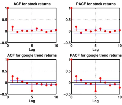
3.4 ACF and PACF of stock returns and GT returns . . . 52

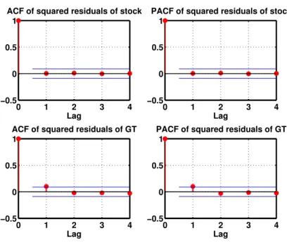
3.5 ACF and PACF of the squared residuals of the stock returns and GT returns . . 53

3.6 Normalized weekly Influenza-Like Illness (ILI) data and Google Trends (GT) data (from Jan. 4 2004 to Feb. 8 2015). . . 55

(14)

4.1 Distributed classification using a wireless sensor network . . . 63 4.2 Pcvs. SNR for testing between two PSK modulation schemes . . . 83

4.3 Pcvs. SNR for testing a PSK against a QAM . . . 84

4.4 Pcvs. SNR for testing BPSK against QPSK in sensor networks with different

sizes . . . 85 4.5 Pcvs. SNR for 3 hypotheses testing . . . 85

5.1 Characteristic functions ofX andY . . . 105 5.2 ROCs corresponding to different fusion rules in a 2-sensor network withβ =

0.35. . . 109 5.3 ROCs corresponding to different copula libraries withβ = 0.3: Frank copula

is used to generate the data, GLRT without misspecification corresponds to the case whereC ={Gaussian, Gumbel, Clayton, Frank}, while GLRT with mis-specification corresponds to the case whereC ={Gaussian, Gumbel, Clayton}. 110 5.4 PD as a function of censoring rateβunderScenario A-CandScenario Q-C . 111

5.5 ROCs corresponding to different fusion rules in a multi-sensor network with

β = 0.25. . . 112 6.1 GAFI corresponding to Gaussian copula vs. correlation coefficient ρ. The

marginal distributions are Gaussian with mean θ1 = θ2 = 1 and variance

σ2

1 =σ22 = 4for the identical case;σ12 = 4, σ22 = 1for the heterogeneous case. . 124

6.2 GKLD corresponding to different copulas vs. Kendall’sτ. Gaussian marginals are assumed. Means are assumed to beθ1 =θ2 = 2underH0 andθ1 =θ2 = 1

underH1. Variances are assumed to beσ12 = 4, σ22 = 1under both hypotheses. . 131

(15)

6.4 The deployment of the 8-sensor network and the final partition. . . 142 6.5 The overall payoff vs. number of merge/split operations for different

initializa-tion of the merge-and-split algorithm. . . 143 6.6 Overall estimation performance vs. communication constraintα. . . 145 6.7 Overall actual communication cost vs. communication constraint α in

esti-mation problem. (The curves for Coalition Foresti-mation under IA and Random Coalition Formation are overlapped.) . . . 146 6.8 Overall detection performance vs. communication constraintα. . . 147 6.9 Overall actual communication cost vs. communication constraintα in

detec-tion problem. (The curves for Coalidetec-tion Formadetec-tion under IA and Random Coalition Formation are overlapped.) . . . 148

(16)

C

HAPTER

1

I

NTRODUCTION

The problem of inferring events of interest by fusing data from multiple sensors has a wide variety of applications ranging from the surveillance of borders to disaster management. The inference tasks could consist of detecting an activity of interest or estimating some parameters, such as locations or tracks, that provide information for situational awareness. The sensors de-ployed in a given region of interest, in the most general setting, may consist of rather disparate and incommensurate modalities. In other words, with respect to the information content of the signals, sensors exhibit heterogeneity that can arise from a wide variety of causes. Another factor that influences the performance of such a multisensor system is the fact that the sensors observe different aspects of the same phenomenon, i.e., sensor observations are dependent. The nature of this dependence can be quite complex and nonlinear, especially in cases where the signal may propagate through a non-homogeneous medium. Inference in such a multisensor system is the major topic of this thesis.

Social media, facilitated by the growth of social networks, provides an easily accessible platform for users to share information and has resulted in the generation of unprecedented amounts of social media data that can be recorded and even monitored (such as, wall posts, clicks etc). This massive amount of social media data can be used by the signal

(17)

process-ing community, in combination with sensor data, for extractprocess-ing information about unfoldprocess-ing events. This is expected to be beneficial in the military as well as civilian domains and pro-vides us the motivation to investigate the convergence of sensor networks and social media in facilitating the data-to-decision making process and study how the two systems can comple-ment each other for enhanced situational awareness. In networks with limited communication resources, local observations are usually compressed according to certain local rules, and only the compressed information is transmitted to the FC. In such distributed networks, the mecha-nism at sensors that is applied to reduce transmission can be quantization, censoring, etc. The existence of nonlinear inter-sensor dependence and heterogeneity of the network make the de-sign of local rules and the fusion rule highly complex. We study the dede-sign of local and fusion rules in this thesis, which take inter-sensor dependence into consideration to improve inference performance. Local collaboration in the form of non-overlapping coalitions is also investi-gated to explore the dependence among sensors so that inference performance is improved to the largest extent under limited communication budget.

1.1 Background

Copula theory, which forms the basis of a lot of work in this thesis, is presented in this section.

1.1.1 Copula Theory

Copulas are parametric functions that couple univariate marginal distributions to a multivariate distribution. They can model the dependence among random variables with arbitrary marginal distributions. An important theorem that is central to the theory of copulas is Sklar’s theorem (see Nelsen [75] for a detailed proof), which is stated below.

Theorem 1.1 (Sklar’s Thoerem). Consider an N-dimensional distribution function F with marginal distribution functions F1, . . . , FN. Then there exists a copula C, such that for all

(18)

F(x1, x2, . . . , xN) =C(F1(x1), F2(x2), . . . , FN(xN)) (1.1)

If Fn is continuous for1 ≤ n ≤ N, thenC is unique, otherwise it is determined uniquely on

RanF1×. . .×RanFN whereRanFnis the range of cumulative distribution function (CDF)

Fn. Conversely, given a copulaC and univariate CDFsF1, . . . , FN, F as defined in Eq.(1.1)

is a valid multivariate CDF with marginalsF1, . . . , FN.

Note that Eq. (1.1) implies that the copula function is a joint distribution of uniformly distributed random variables. As a direct consequence of Sklar’s Theorem, for continuous distributions, the joint probability density function (PDF) is obtained by differentiating both sides of Eq. (1.1), f(x1, . . . , xN) = _YN n=1 f(xn) c(F1(x1), . . . , FN(xN)) (1.2)

where,cis termed as the copula density and is given by,

c(u) = ∂ N₍_C₍_u 1, . . . , uN)) ∂u1, . . . , ∂uN (1.3) where,un =Fn(xn).

Thus, we can construct a joint density function with specified marginal densities by employ-ing Eq. (1.2). Note thatC(·)is a valid CDF andc(·)is a valid PDF for uniformly distributed random variables, un. The choice of a copula function to represent the joint statistics of the

sensor observations is an important consideration here. Various families of copula functions exist in the literature [75]. However, which copula function should be used for a given case is not very clear as different copula functions may characterize different types of dependence behavior among the random variables [69]. A brief summary of some popularly used copula

(19)

functions is provided next.

1.1.2 Summary of Some Copula Functions

Copulas derived from distributions

Multivariate distribution functions specify dependence structures and copula functions can be derived from them. Two such copula functions are the Gaussian and thetcopula functions that are derived from multivariate Gaussian and Student-t distributions respectively. Both specify dependence using the correlation matrix and are given as follows.

The Gaussian copula is defined as

CG(u|Σ) = ΦΣ(Φ−1(u1), . . . ,Φ−1(uN)), (1.4)

where, ΦΣ denotes the multivariate normal CDF and Φdenotes the univariate normal CDF.

Similarly, thet-copula is defined as

Ct(u|Σ, ν) =tν,Σ(tν−1(u1), . . . , t−ν1(uN)) (1.5)

where, tν,Σ is the multivariate Student-t distribution with correlation matrix Σand ν degrees

of freedom (ν ≥ 3) and tν denotes the univariate Student-t distribution with ν degrees of

freedom. It is common to setν = 3to incorporate heavy tail dependence. Asν → ∞,thet

copula approaches the Gaussian copula function. Both the Gaussian and thetcopula functions belong to the elliptical family of copulas.

(20)

Clayton _φ1 u−φ−1 PN

n=1u −φ

n −1 , φ∈[−1,∞)\{0}

Frank −log exp_exp{−φu}−_{−φ}−₁1 −1 φlog 1 + QN n=1[exp{−φun}−1] exp{−φ}−1 , φ∈_R\{0} Gumbel −lnuφ _exp −PN n=1(−lnui)φ _φ1 , φ∈[1,∞) Independent −lnu QN n=1un Archimedean copulas

Archimedean copulas, describing anm-variate CDF, are defined as follows,

C(u|φ) = Ψ−1 N X n=1 Ψ(un) ! (1.6)

where, Ψ(·)is referred to as the generator function andφ is the copula parameter specifying dependence. The Archimedean copulas considered in the chapters to follow are shown in Table 1.1 (see [75]).

1.1.3 Copulas and Measures of Dependence

An attractive feature of copulas is that nonparametric rank-based measures of dependence, such as Kendall’sτ, can be expressed as expectations over the copula distribution. For independent pairs of random variables(X1, Y1)and(X2, Y2)having the same distribution as(X, Y),

con-cordance is defined as the condition that(X1−X2)(Y1−Y2)≥0and discordance is defined as

the condition that(X1−X2)(Y1−Y2)<0. Kendall’sτis defined to be the difference between

the probabilities of concordance and discordance:

(21)

Nelsen has proved the relationship in (1.7) for a copula, C, and random variables X ∼

fX(x), Y ∼fY(y)[75, p. 161], i.e.,

τ(φ) = 4_E[Cφ(FX(x), FY(y))]−1. (1.7)

This relationship allowsτ to be expressed in terms of the dependence parameter of the copula,

C (Σfor the elliptical copulas and φfor the Archimedean copulas in Table 1.1). For the case of elliptical copulas, parametrized by the matrixΣ = [ρmn],

ρmn = sin

πτ_mn

2

, (1.8)

whereτmnis the Kendall’sτ evaluated for the pair(Um, Un) = (FXm(·), FXn(·)). The sample

estimate of Kendall’s τ, for N observations, can be calculated as the ratio of the difference in the number of concordant pairs,c, and discordant pairs, d, to the total number of pairs of observations, i.e., ˆ τ = c−d c+d = c−d N 2 (1.9)

Typically, the value of the dependence parameter is not known a priori, and φ needs to be estimated, e.g., using maximum likelihood estimation (MLE). On the other hand, (1.9) and (1.7) imply that Kendall’sτ can be used for calculating computationally efficient estimates of

φ.

1.2 Literature Review

Multisensor signal processing may be viewed as a subset of the broader field of information fusion. Centralized formulations, where raw observations are available at the processing unit or fusion center, for several inference tasks are well known and available in standard text-books [14, 61, 107]. Distributed inference, on the other hand, relies on the availability of a

(22)

While research in this area has forked in various directions, the problems addressed can be cat-egorized as either distributed detection [114] or decentralized estimation (e.g., see [76, 78, 84] and references cited therein).

This section reviews recent progress that has been made in the field of multisensor signal processing, and focuses on developments where dependence information plays a significant role in the design. The aim of the discussion, as presented, is to motivate the relevance of our current research. The emphasis on dependence notwithstanding, the literature is quite exten-sive, and instead of being exhaustive, we concentrate on highlighting newer developments.

1.2.1 Dependence as Covariance

Modeling dependence as a covariance matrix (or equivalently a correlation matrix) is arguably one of the most popular ways of characterizing dependence. It defines the dependence of jointly normal random variables and describes the linear dependence between random variables that possess a finite second moment. In the centralized paradigm, it is used extensively to model the dependency information for array signal processing applications, especially where it is rea-sonable to assume linearity of the medium of signal propagation. The most recent technologies where these concepts of array signal processing have been applied are MIMO radar [67] and joint blind source separation (JBSS) [5]. In MIMO radar, several antenna elements are used to transmit multiple probing signals that may be correlated or uncorrelated with one another. While traditional blind source separation problems are formulated using a single dataset, JBSS formulations are useful when analyzing multiple datasets as a group. An example of this is the separation of speech and audio signals in multiple frequency bands. The fusion of EEG with fMRI data for the detection of schizophrenia is discussed by Correa et al. [26] where the brain tissue is modeled as a mixing channel, and hence the information fusion problem is posed as

(23)

a JBSS problem and is solved using an approach based on multivariate canonical correlation analysis [62]. Canonical correlation analysis (CCA) has also been used for audio-video fusion: Slaney and Covell [93] use CCA to measure the synchrony between acoustic features and video frames, while Kidron et al. [63] consider a CCA based approach to determine pixels in images that exhibit maximal correlation with the acquired audio signal.

Optimal schemes for distributed inference with correlated observations has also been a topic of considerable interest. In the case of distributed detection, it has been shown that the likelihood ratio based quantizer, which was optimal under the assumption of conditional in-dependence, is no longer optimal when correlation is taken into account. Examples of the consequent loss in performance are provided by Aalo and Viswanathan [1]. In fact, earlier work by Tsitsiklis and Athans [111] has shown that the distributed detection problem with de-pendent observations is NP-complete. One way to get past the computational intractability is to assume some prior knowledge about the joint statistics: Drakopolous and Lee [33] examine the fusion rule for distributed detection under dependence by considering that the correlation coefficient is known, whereas Kam et al. [58] use the Bahadur-Lazarsfeld expansion of prob-ability density functions. Willett et al. [123] study the problem of distributed detection of a mean shift in correlated Gaussian noise and establish how the nature of correlation affects the optimum fusion rule. They conclude that even for a simple two-sensor and linear correlation formulation the distributed detection problem “exhibits apparently very complicated behavior." The decentralized estimation problem with correlated observations has been studied by Fang and Li [39]. They consider a power constrained wireless sensor network [104] and ex-amine power allocation for spatially correlated sensor observations. Each sensor transmits a possibly nonlinear function of the parameter of interest,θ, that is corrupted by additive, corre-lated Gaussian noise. Bandwidth constrained formulations requiring quantized transmissions to the fusion center are also considered by Ribeiro and Giannakis [84]. However, they con-sider a linear observation model, withθbeing deterministic but unknown, and hence the sensor

(24)

the noisewn is a multivariate Gaussian correlated spatially across sensors. The covariance is

assumed to be known at the fusion center. We note that all these problems are considered to be distributed since each local sensor transmits some local estimate ofθ, which in its simplest form is the noise corrupted parameter itself. These formulations do not consider local, inter-node communication; the implications of this local communication aspect have been recently investigated by Kar et al. [60].

1.2.2 Nonlinear Dependence: Nonparametric Approach

Nonparametric approaches to multisensor signal processing have been very popular in applica-tions where it is infeasible to modela priorithe complex dependencies that may exist between the signals/features acquired by the sensors. These methods, in essence, estimate or learn the joint distribution across sensor measurements directly from the data.

Machine learning techniques fall under this framework and are applicable largely when it is feasible to control environment variables in such a way that a representative training dataset may be collected. While this is apparently a stringent requirement, often with some prepro-cessing, a significant amount of information can be extracted from sensor observations. This has led to the successful application of machine-learning techniques for a wide variety of prob-lems. Learning based methodologies have been successfully applied to multibiometric sys-tems [12, 85]. Multibiometric syssys-tems achieve superior personnel identification performance by fusing information from two or more biometric modalities. The learning-based approach has also been popular for solving several object classification tasks [57,73] and have tradition-ally focused on security and surveillance applications [66, 132]. Recently, challenges unique to emerging technologies such as ubiquitous and human-centered computing have led to new research in areas such as object tracking and affect recognition [125, 128].

(25)

When viewed from an information fusion perspective, nonparametric designs offer tangible advantages over methods described in Section 1.2.1. Fusion of heterogeneous or multimodal information is possible since disparate modalities are not constrained to a multivariate normal approximation. For example, Butz and Thiran [18] use the mutual information and joint en-tropy between audio and video data as a measure of dependence; the joint density required for the computation of these quantities is estimated from the data using the nonparametric Parzen’s estimator [119]. Graphical models such as Bayesian networks generalize hidden Markov mod-els and have also been successfully used for audio-visual tracking [11, 28, 57]. Algorithms for distributed fusion using graphical models have been described by Çetin et al. [19].

1.2.3 Nonlinear Dependence: Copula-based Approach

Recall from Section 1.1.1 that copulas are parametric functions that couple univariate marginal distribution functions to the corresponding multivariate distribution function. A copula-based formulation is attractive because the spatial correlation among sensor observations can get manifested in several different, potentially non-linear ways and many families of copula func-tions have been specified in the literature to address this issue. Further, while nonparametric formulations are known to converge to the true distribution asymptotically, they also suffer from scalability issues stemming from the curse of dimensionality. Recently, considerable progress has been made in the study of copulas and their applications in statistics. The usage of copulas is widespread in the fields of econometrics and finance [25] and they are beginning to be used in the signal and image processing context [29, 52, 71, 103].

Iyengar et al. [51] have investigated the general framework of copula-based detection of a phenomenon being observed jointly by heterogeneous sensors. They quantify the performance loss due to copula misspecification and demonstrate that a detector using a copula selection scheme based on area under the receiver operating characteristic (ROC) can provide signifi-cant improvement over models assuming independence. Their results on a NIST

(26)

multibiomet-et al. [100] consider the case of distributed dmultibiomet-etection and derive the optimum fusion rules for a Neyman-Pearson detector. Sundaresan and Varshney [99] also design and analyze the perfor-mance of a copula-based estimation scheme for the localization of a radiation source.

1.3 Main Contributions and Organization

The main contributions of the research results presented in this dissertation to the signal pro-cessing and information fusion literature, are as follows:

In Chapter 2, we investigate the detection problem using heterogeneous sensor data, where observations from disparate sensors may be conditionally dependent. We use copula theory to construct a valid joint distribution, to describe the dependence among these heterogeneous data. We consider the dependence to be “complex", where the “complexity" is assumed to include two cases, one is when the dependence structure is non-stationary, the other is when the true dependence is beyond the description of a single copula. For the scenario of non-stationary dependence, we propose a sample-wise copula selection rule and theoretically justify its utility. For the other scenario, we use a mixture of copulas to approach the true underlying dependence and use expectation maximization (EM) algorithm to solve for the unknown parameters in the model. Both theoretical proofs and simulation results are provided to show that the mixture of copula model results in a better detection performance compared with previously used single copula method. We also apply our proposed approaches to personnel detection using real footstep data collected by acoustic and seismic sensors.

The access to the massive amount of social media data provides a unique opportunity to the signal processing community for extracting information that can be used to infer about

(27)

unfolding events. It is desirable to investigate the convergence of sensor networks and social media in facilitating the data-to-decision making process and study how the two systems can complement each other for enhanced situational awareness. In Chapter 3, we propose a copula-based joint characterization of multiple dependent time series from sensors and social media. As a proof-of-concept, this model is applied to the fusion of Google Trends (GT) data and stock price data of Apple Inc. for prediction, where the stock data serves as a surrogate for sensor data. We also apply our model to the fusion of GT data and Influenza-Like Illness (ILI) data from Centers for Disease Control and Prevention (CDC) for flu prediction. Superior prediction performance of our method is demonstrated for both problems, by taking the non-linear dependence among social media data and sensor data into consideration.

In Chapter 4, we consider the distributed classification of discrete random signals in wire-less sensor networks (WSNs). Observing the same random signal makes sensors’ observations conditionally dependent which complicates the design of distributed classification systems. In the literature, this dependence has been ignored for simplicity although this may significantly affect the performance of the classification system. We derive the necessary conditions for the optimal decision rules at the sensors and the fusion center (FC) by introducing a “hidden" random variable. Furthermore, we introduce an iterative algorithm to search for the optimal decision rules, the convergence of which is also proved. The proposed scheme is applied to a distributed Automatic Modulation Classification (AMC) problem. It is shown to attain superior performance in comparison with other approaches which disregard the inter-sensor dependence.

In Chapter 5, we consider a distributed detection problem for a censoring sensor network where each sensor’s communication rate is significantly reduced by transmitting only “infor-mative" observations to the Fusion Center (FC), and censoring those deemed “uninfor“infor-mative". Our focus is on designing the fusion rule under the Neyman-Pearson (NP) framework that takes into account the spatial dependence among observations. Two transmission scenarios are

(28)

Copula-based Generalized Likelihood Ratio Test (GLRT) for censored data is proposed with both continuous and discrete messages received at the FC corresponding to different transmis-sion strategies. We address the computational issues of the copula-based GLRTs involving multidimensional integrals by presenting more efficient fusion rules, based on the key idea of injecting controlled noise at the FC before fusion. Although, the signal-to-noise ratio (SNR) is reduced by introducing controlled noise at the receiver, simulation results demonstrate that the resulting noise-aided fusion approach based on adding artificial noise performs very closely to the exact copula-based GLRTs. Copula-based GLRTs and their noise-aided counterparts by exploiting the spatial dependence greatly improve detection performance compared with the fusion rule under independence assumption.

We consider the problem of collaborative inference in a sensor network with heteroge-neous and statistically dependent sensor observations. Each sensor aims to maximize its in-ference performance by forming a coalition with other sensors and sharing information within the coalition. In Chapter 6, the formation of non-overlapping coalitions with statistically de-pendent sensors is investigated under a communication constraint. We apply a game theoret-ical approach to fully explore and utilize the information contained in the spatial dependence among sensors to maximize individual sensor performance. Before formulating the distributed inference problem as a coalition formation game, we quantify the gain and loss in forming a coalition by introducing the concepts ofdiversity gainandredundancy lossfor both estimation and detection problems. These definitions, enabled by the statistical theory of copulas, allow us to characterize the influence of statistical dependence among sensor observations on infer-ence performance and collaboration strategy. An iterative algorithm based on merge-and-split operations is proposed for the solution and the stability of the proposed algorithm is analyzed. Numerical results are also provided for illustration.

(29)

Finally, in Chapter 7, we summarize the findings and results of this dissertation. Several directions and ideas for future research are also presented.

1.4 Bibliographic Note

Part of the work presented in this dissertation has appeared in the following publications:

1. Hao He, Arun Subramanian, Pramod K. Varshney, and Thyagaraju Damarla, “Fusing Heterogeneous Data for Detection Under Non-stationary Dependence," in Proc. 15th International Conference on Information Fusion, 2012.

2. Hao He, Arun Subramanian, Xiaojing Shen, and Pramod K. Varshney, “A Coalitional Game for Distributed Estimation in Wireless Sensor Networks," inProc. IEEE Interna-tional Conference on Acoustics, Speech, and Signal Processing (ICASSP), 2013.

3. Hao He, and Pramod K. Varshney, “Distributed Detection with Censoring Sensors under Dependent Observations," inProc. IEEE International Conference on Acoustics, Speech, and Signal Processing (ICASSP), 2014.

4. Hao He, Sora Choi, Pramod K. Varshney, and Wei Su, “Distributed Classification un-der Statistical Dependence with Application to Automatic Modulation Classification," in

Proc. 18th International Conference on Information Fusion, 2015.

5. Hao He, Arun Subramanian, Sora Choi, Pramod K. Varshney, and Thyagaraju Damarla, “Social Media Data Assisted Inference with Application to Stock Prediction," to appear inProc. IEEE Asilomar Conference on Signals Systems and Computer, 2015.

6. Hao He, and Pramod K. Varshney, “Fusing Censored Dependent Data for Distributed Detection," Signal Processing, IEEE Transactions on, vol 63, no. 16, pp. 4385-4395, Aug. 15, 2015.

(30)

(31)

C

HAPTER

2

C

ENTRALIZED DETECTION UNDER

COMPLEX DEPENDENT OBSERVATIONS

2.1 Motivation

Fusion of data from heterogeneous sources of information, observing a certain phenomenon, has been shown to improve the performance of several inference tasks. Sensors are said to be heterogeneous if their respective observation models cannot be described by the same proba-bility density function (PDF) [51]. Naturally, an information fusion system comprising multi-modal sensors satisfies this definition. However, sensors of the same multi-modality too can be het-erogeneous, in the sense defined here, as they may span varied deployment and manufacturing conditions.

In this chapter, we consider centralized detection in the Neyman-Pearson (NP) framework with heterogeneous dependent observations for two cases. The first one is when the depen-dence is non-stationary where the non-stationarity is assumed to manifest itself as time-varying spatial dependence across the sensors. This is a plausible situation, especially in multi-modal deployments: based on the physics governing the individual modalities, transient phenomena

(32)

same observation window. In other words, for reasonably short observation windows, the sig-nal from a single modality can be modeled as a quasi-stationary process, an approach that has been used extensively in spectral analysis and statistical signal processing [36, 70]; modeling cross-sensor dependence, on the other hand, would require a more considered approach. The other case is when the true dependence is beyond the description of any single copula. Un-der such circumstances, using a single copula to represent the true dependence structure will introduce model mismatch error and lead to suboptimal performance [50]. Thus, a mixture of copulas model which is able to approach the true dependence in multiple directions can be used . A mixture of copulas is usually more flexible compared with single copula models due to an increase in the number of parameters, thus resulting in more degree of freedom and a better performance in describing the dependence among observations.

2.2 Problem Formulation

Consider a scene or phenomenon being monitored by a sensor suite, consisting ofN sensors. Thenth sensor, n = 1,2, . . . , N, makes a set of L measurements, xnl, l = 1. . . , L. These

measurements may represent a time series (with l being the time index), spectral coefficients (with l being the frequency index), or some other feature vector. The vector xl denotes the

l-th measurements at all the sensors, i.e., xl = [x1l, . . . , xN l]T. The collective measurements, x = [x1, . . . ,xL], are received at a processing unit or Fusion Center (FC). Based on the joint

(33)

of interest and, thus, solves the following hypothesis testing problem: H0 :f(x|H0) = L Y l=1 f(xl|H0) H1 :f(x|H1) = L Y l=1 f(xl|H1), (2.1)

whereH0 is the null hypothesis that the background process is observed, and H1 is the

alter-native, i.e., the phenomenon of interest is observed. The PDFs under the null and alternative hypotheses are, respectively, denoted asf(·|H0)andf(·|H1). In taking the product over all l

in (2.1), we assume that for a given sensor, signals are independent over the indexl, e.g., over time. However, in general,

f(xl|Hi)6= N

Y

n=1

fn(xnl|Hi), i= 0,1 (2.2)

wherefn(xn|H0)andfn(xn|H1), respectively denote the PDFs of sensorn’s observations

un-der hypotheses H0 and H1. This formulation, therefore, asserts that since the sensors are

observing the same phenomenon, at any given instant, sensor measurements need not be inde-pendent spatially (across sensors).

Using Sklar’s theorem (Section 1.1.1, Theorem 1.1), the joint densities in (2.1) can be expressed in terms of the copula densities,c0andc1, respectively underH1 andH0, as,

f(x|Hi) = L Y l=1 " _N Y n=1 fn(xnl|θin, Hi) ! ci(ui1l(θi1), . . . , uiN l(θiN)|φi) # , i= 0,1 (2.3) The copula arguments are the probability integral transforms (PIT) ofxnl under hypothesisHi,

i.e., for sensornand measurementl,

(34)

test (LRT) is the optimal test. Equivalently, we can compare the log-likelihood ratio (LLR) to a thresholdη, TLR(x) H1 ≷ H0 η, (2.5) where, TLR(x) = log f(x|H1) f(x|H0) = L X l=1 N X n=1 logfn(xnl|θ1n, H1) fn(xnl|θ0n, H0) + L X l=1 logc1(u 1 1l(θ11), . . . , u1N l(θ1N)|φ1) c0(u01l(θ01), . . . , u0N l(θ0N)|φ0) (2.6)

These parameters{θ0,θ1}and{φ0,φ1}are typically unknown and have to be estimated.

Using maximum likelihood (ML) estimates in place of the true parameter values, the test be-comes a generalized likelihood ratio test (GLRT) in the Neyman-Pearson framework. From (2.3) and (2.4), it is seen that the copula density is also a function of the marginal parameter,

θin, through the PIT. Thus, ideally, ML estimation of the parameters would require

simultane-ous maximization of the joint likelihood function over both, the marginal and copula param-eters. This is, however, difficult and a consistent two-step estimation procedure is commonly used in the copula literature [108]. The two-step maximum likelihood (TSML) procedure first maximizes the individual marginal likelihoods over eachθin:

b θin= arg max θin L X l=1 logfn(xnl|θin, Hi) (2.7)

(35)

is then maximized overφ_i, i.e., b φ_i = arg max φi L X l=1 logci(ˆui1l, . . . ,uˆ i N l|φi). (2.8) whereuˆi

nl =uinl(bθ_in). The GLRT then can be expressed as, TGLR(x) H1 ≷ H0 η, (2.9) where, TGLR(x) = L X l=1 N X n=1 log fn(xnl|bθ1n, H1) fn(xnl|bθ₀_n, H₀) + L X l=1 logc1(u 1 1l(bθ₁₁), . . . , u1_{N l}(bθ₁_N)|φb₁) c0(u0₁_l(bθ01), . . . , u0_{N l}(bθ0N)|φb₀) (2.10)

Alternatively, for the bivariate case (N = 2), we can also use the sample estimate of Kendall’s τ, defined in (1.9), to estimate φ_i. Noting that the relation in (1.9) is invertible, we rewrite the function relationship betweenτandφ_iin (1.7), in terms of a functiongiso that,

φ_i =g_i−1(τ).The resultant estimate ofφ_iis given by

e

φ_i =g_i−1(ˆτ). (2.11)

In multivariate copulas, such as Gaussian copula, the dependence parameter is a matrix where each element is the correlation coefficient of two random variables and can be associated with the corresponding pairwise τ. In other forms of multivariate copulas, such as the ones con-structed through a vine [65, 97], (conditional) bivariate copulas are the basic elements of the structure, whose associated parameters are directly related to the corresponding (conditional) pairwiseτ.

Further, sinceτˆis a consistent estimator ofτ [42],φe_i →φ_i asL→ ∞. For finiteL, using e

(36)

preceding section assumes that the family of copulas,c0andc1, are known, a formulation with

non-stationary dependence has to necessarily drop that assumption. In the following discus-sion, we assume that the background model can be predetermined to some degree: the family of the marginals is known andc0is known. The more general case of unknownc0is considered

by Iyengar et al. [51], but signal detection for such a scheme need to be implemented under a training-testing paradigm. However, non-stationarity notwithstanding, the true underlying copula underH1, c, is typically not known; this “true copula” is usually abstracted as a single

copula, but it may, in fact, be a composite of several copulas interacting in an indeterminate fashion, accounting for the non-stationary nature of observations. Due to these complexities, copula selection is an important part of copula based inference and several copula selection methods have been proposed [51, 97, 103]. Our assumptions are stated more precisely as fol-lows:

1. We assume that fn(·|H0), the marginal density families under H0, are known for each

n = 1, . . . , N. The corresponding marginal parameters,θ0n, may be unknown.

2. The H0 copula family, c0, is known but φ0 may be estimated, if needed. This section,

however, assumes, without loss of generality, thatc0 = 1, i.e., measurements underH0

are independent across sensors. However, the discussion is valid for any knownc0. The

independence under the null hypothesis also allows us to simplify our notation; we do not explicitly notate forH1 with respect to the copula function. Therefore, we set

c1(·)≡c(·)

u1_nl(θin)≡unl

(37)

3. The copula under the alternative, c1, is not known a priori. The “best” copula, in the

sense of maximum likelihood, is selected from a predefined library of copulas, C =

{cm :m= 1, . . . , M}.

Based on these assumptions, we discuss three detection scenarios: detection with known parameters, detection with unknown parameters, and detection with unknown marginals under

H1 and unknown copula parameters.

2.3.1 Detection with Known Parameters

For some applications, it may be feasible to determine,a priori, the value of the copula param-eterφ_mfor eachcm ∈ C. The actual selection of the copula may be done online. For this case

the test-statistic is formulated as a modification of (2.6),

where for eachlthe maximum copula likelihood is selected from the libraryC, i.e.,

c∗_l = arg max

cm∈C

cm(u1l, . . . , uN l|φ∗l) (2.13)

The key difference here is that previous work has proposed the scheme of selecting a single copula for the entire observation window [51, 97], i.e., choose a single copulac∗_L

c∗_L= arg max cm∈C L X l=1 logcm(u1l, . . . , uN l|φ∗L) (2.14) for all l = 1, . . . , L. On the other hand, we select the best copula for each l adapting to

(38)

our assumptions,H0) is known, it has been shown that [37] the loss in detection power defined

as

∆loss =

Z

PD(η)−PˆD(η)dη (2.15)

when fX(·|H1) is misspecified as fˆ(·|H1), is equal to the Kullback-Leibler (KL) divergence

D(fX(·|H1)||fˆ(·|H1)). We now prove that selecting the best copula for eachl, as opposed to

a single best copula for allL, leads to a smaller KL divergence from the single true copula, c

and thus a better performance in terms of loss in detection power.

Proposition 2.1. LetX∼f(x|H1),X∈RL×N, where,

fX(x|H1) = L Y l=1 " _N Y n=1 fn(xnl|θ1n, H1) ! c(u1l, . . . , uN l|φ) # (2.16)

where cis the true copula. For the copula library,C = {cm : m = 1, . . . , M},and selection

schemes(2.13)and(2.14),

D(fX||fc∗_l)≤D(fX||fc∗_L), (2.17)

wherefc∗_l andfc∗_L are the joint densities forXunderH1using(2.13)and(2.14)respectively.

Proof. Consider the caseM = 2. Choosingc1overc2whenc1(u1l, . . . , uN l)≥c2(u1l, . . . , uN l)

is equivalent to the decision rule when copula selection is posed as a decision problem with equally likely copulas. LetΩrepresent the sample space. LetΩm ⊂ Ωrepresent the decision

region forxfor whichcm(m= 1,2)is chosen, so thatΩ1∪Ω2 = ΩandΩ1∩Ω2 =∅. Denote

the product of marginals asfp(xl), i.e.,

fp(xl) = N

Y

n=1

(39)

Also, define the following sets: J1 ={l:xl∈Ω1}andJ2 ={l:xl ∈Ω2}. Then, D(fX||fc∗_l) = Z log fX(x) fc∗_l(x) dFX = Z log L Q l=1 fp(xl)c(u1l, . . . , uN l|φ) L Q l=1 fp(xl) Q J1 c1(·|φ1) Q J2 c2(·|φ2) dFX = Z L X l=1 logc(·)dFX − Z " X J1 logc1(·) + X J2 logc2(·) # dFX (2.19)

The selection criterion in (2.13), implies that, for the setJ2,c2 ≥c1. Therefore,

X J1 logc1(·) + X J2 logc2(·)≥ X J1 logc1(·) + X J2 logc1(·) = L X l=1 logc1(·), (2.20)

and in a similar manner,

X J1 logc1(·) + X J2 logc2(·)≥ L X l=1 logc2(·) (2.21)

Therefore, depending on whetherc1orc2was chosen using (2.14), we can substitute either of

the inequalities in (2.20) and (2.21) in (2.19) to get,

D(fX||fc∗

l)≤D(fX||fc ∗

(40)

true dependence to becfor all time instantsl. Since the true copula appears only in the first term of (2.19), which is irrelevant to the copula selection rule, the proof holds for any type of true dependence (time invariant, or time varying).

Proposition 2.1 implies that a detector using the selection scheme proposed in (2.13) will suffer a lower loss in detection performance due to copula misspecification [51].

2.3.2 Detection with Unknown Parameters

With unknown parameters, the statistic in (2.10) for the composite hypothesis testing problem can be rewritten as,

TGLR(x) = L X l=1 N X n=1 log fn(xnl|θb1n, H1) fn(xnl|θb0n, H0) + L X l=1 logc∗_l(u1l(θb₁₁), . . . , u_{N l}(θb₁_N)|φb ∗ l), (2.22)

where the TSML procedure has been used to obtain estimates of marginal and copula parame-ters. The copula parametersφb_mare estimated overL, for eachc_m ∈ C, so that

C ={cm(·|φb_m(L)) :m= 1, . . . , M} (2.23) c∗_l = arg max cm∈C logcm(u1l(bθ₁₁), . . . , u_{N l}(bθ₁_N)|φb_m(L)) (2.24) b φ∗_l = argc∗_l (2.25) While this selection method is motivated by the implications of Proposition 2.1 for the simple hypothesis case, a similar result may not be stated for the composite test. This is because ML estimation requires that allLsamples be drawn from the same population; this need not hold

(41)

true for copula selection fromC with unknown parameters. The copula parameters can also be estimated using Kendall’sτˆ. The test-statistic is then,

Tˆτ(x) = L X l=1 N X n=1 log fn(xnl|bθ1n, H1) fn(xnl|bθ₀_n, H₀) + L X l=1 logc∗_l(u1l(bθ₁₁), . . . , u_{N l}(bθ₁_N)|φe ∗ l), (2.26) whereφe ∗ l is the estimate ofφ ∗ l based onτˆ. Correspondingly, C ={cm(·|φm(ˆτ)) :m= 1, . . . , M} (2.27) c∗_l = arg max cm∈C logcm(u1l(bθ11), . . . , uN l(bθ1N)|φm(ˆτ)) (2.28) e φ∗_l = argc∗_l (2.29)

2.3.3 Detection with Unknown Marginals and Unknown Copula

Pa-rameters

In many applications, establishing a model under H1 is not feasible. In that case, fn(·|H1)

is determined non-parametrically and uij is obtained using the empirical probability integral

transform (EPIT). The test statistic is, therefore, expressed as,

TNPM(x) = L X l=1 N X n=1 log ˆ fn(xnl|H1) fn(xnl|bθ₀_i, H₀) + L X l=1 logc∗_l(ˆu1l, . . . ,uˆN l|φb ∗ l), (2.30)

(42)

ˆ Fn(·|H1) = 1 L L+1 X l=1 1xnl<{·} (2.31) ˆ unl = ˆFn(xnl|H1) (2.32)

where1{·} is the indicator function.

The marginal model underH1is determined through a kernel density estimation procedure.

Kernel density estimators [119] provide a smoothed estimate,fˆn(xnl|H1), of the true density.

Choosing the correct bandwidth for kernel density estimation is important for an accurate es-timate. The kernel bandwidth is chosen using leave-one-out cross-validation. The selected bandwidth, h∗, is the minimizer of the cross-validation estimator of risk, Jˆ, for a kernel, K. The risk estimator may be easily computed using the approximation [119, p. 136],

ˆ J(h) = 1 hN2 X p X q K∗ Xp−Xq h + 2 N hK(0) +O 1 N2 , (2.33) where, K∗(x) =K(2)(x)−2K(x) K(2)(z) = Z K(z−y)K(y)dy.

The Gaussian kernel is used in this work, so thatK(x) =N(x; 0,1)andK(2)₍_z_{) =} _N₍_z_{; 0}_,₂₎_.

Therefore,

h∗ = arg min

h

ˆ

(43)

2.4 Detection Using Mixture of Copulas

In the previous section, for each sample we chose one copula as the "best" one from the copula libraryC. We actually made the assumption that at each time instant there is an unknown true copula from which the data is generated, thus a hard decision on the best copula is made at each time instant as in a multiple hypothesis testing problem. However, in this section, we assume that every sample is generated bycm with probabilityπm ∈[0,1],∀m = 1, . . . , M, i.e.,

c(·) =

M

X

m=1

πmcm(·|φm), (2.34)

where{cm(·|φm)}are the copula components from libraryC, {πm}Mm=1 are the corresponding

weights satisfyingPM

m=1πm = 1. It has been proved in [75] that (2.34) is also a copula. The

mixture of copulas model provide a more flexible approach to model dependence and can serve as a better descriptor of dependence than a single copula.

The assumptions 1, 2 and 3 that we made in Section 2.3 are still assumed to hold here. According to Sklar’s theorem and the mixed copula in (2.34), the distribution underH1can be

written as f(x) = L Y l=1 " _N Y n=1 fn(xnl|θn) ! × M X m=1 πmcm(u1l(θ1), . . . , uN l(θN)|φm) # . (2.35)

Based on the TSML procedure, marginal parameters can be first obtained by (2.7). Then, after substitutingθn= ˆθn, n= 1, . . . , N, the copula likelihood function is obtained and

maxi-mized over unknown copula parametersφ= (φ1, . . . ,φM)and weightsπ = (π1, . . . , πM).

b π,φb = arg max π,φ L X l=1 log M X m=1 πmcm(ˆu1l, . . . ,uˆN l|φm). (2.36)

(44)

TGLR(x|θb,φb,π_b)≷ H0 η (2.37) where TGLR(x) = L X l=1 N X n=1 logfn(xnl|θb1n, H1) fn(xnl|θb₀_n, H₀) + L X l=1 log M X m=1 ˆ πmcm(ˆu1l, . . . ,uˆN l|φb_m), (2.38)

The superiority of using a mixture copula model, compared with using a single copula model is given in Proposition 2.2: Proposition 2.2. LetX∼f(x),X∈_R1×N , where, fX(x) = " _N Y n=1 fn(xn|θn) ! c(u1, . . . , uN|φ) # (2.39)

wherecis the true copula. AsL→ ∞

D(fX||fc∗

M)≤D(fX||fc

∗), (2.40)

wherefc∗_M andfc∗ are the joint densities forXunderH₁ using mixture of copulas and single

copula respectively.

Proof. Consider the caseM = 2. fp(x)is defined in (2.18). Then,

D(fX||fc∗ M) = Z log fX(x) fc∗_M(x) dFX = Z log fp(x)c(u1, . . . , uL|φ) fp(x)[π1c1(·|φ1) +π2c2(·|φ2)] dFX = Z logc(·)dFX− Z log[π1c1(·|φ1) +π2c2(·|φ2)]dFX (2.41)

(45)

that whenL→ ∞ 1 L L X l=1 log[π1c1(·|φ1) +π2c2(·|φ2)] → Z log [π1c1(·|φ1) +π2c2(·|φ2)]dFX (2.42) So, the second term in (2.41) can be approximated by the sample estimate in (2.42). Since, a single copula model corresponds to a special case of mixture of copulas model in which all the weights are zeros except for one weight that is equal to one, it can be concluded that

max φ1,φ2,π1,π2 1 L L X l=1 log [π1c1(·|φ1) +π2c2(·|φ2)] ≥ max φ1,φ2,πm=1,m=1,2 1 L L X l=1 log [π1c1(·|φ1) +π2c2(·|φ2)] (2.43)

The right hand side of (2.43) correspond to the single copula model. Thus, when L → ∞,

D(fX||fc∗_M)≤D(fX||fc∗)is proved. ForM > 2we can successively arrive at a similar result

by repeating the above steps.

Since there is no explicit analytical expression for the maximum likelihood estimator in (2.36). We use the expectation maximization (EM) algorithm to find the parameters iteratively. The EM algorithm consists of two steps: E-step computes and updates the conditional proba-bility that our observations come from each component copula, and M-step maximizes the log likelihood to estimate the parameters of each copula. LetY ={yl}l=1,...,Lwhose value informs

us as to which component copula “generated" each data item. We assume thatyl ∈ 1, . . . , M

for eachl, andyl = mif the lth sample was generated by themth mixture component. Then

the two steps of the EM algorithm that we developed for the mixture of copula model are as follows:

(46)

whereΘ = (φ,π)is the parameter set and the superscriptrrepresents the fact that the param-eters estimated atrth step. These two steps are repeated until the stopping criterion is satisfied. Each iteration is guaranteed to increase the log-likelihood and the algorithm is guaranteed to converge to a local maximum of the likelihood function [13].

2.5 Results and Discussion

In this section, we present results when the copula-based tests, discussed in Section 2.3, are applied to simulated and real data. Our results are presented for a two-sensor case, i.e.,N = 2. We note, however, that the methods described above apply to more generalized cases as well whereN >2, as one can construct a multivariate copula using bivariate components [97].

2.5.1 Nonstationary Copula

We assume normal and beta distributed marginals respectively and consider various cases of copula dependence. The marginals and the respective parameters used are tabulated in

(47)

Ta-Table 2.1: Distribution of marginals for simulation experiments

n H0 H1

1 N(0,1) N(0.1,1.1)

2 Beta(2.0,2.0) Beta(2.2,2.2)

ble 2.1. For all copula cases we used Kendall’sτ = 0.2to specify the amount of dependence. The copula library contains the Gaussian and Frank copulas, i.e.,C ={Gaussian,Frank}. For all the cases, we compare performances obtained via simulation when performing hypothesis testing with TGLR in (2.22), Tτˆ in (2.26), GLR using single copula selection and the product

rule, i.e., independence assumption. The results presented are averaged over104 _Monte-Carlo

trials with 1000 samples per trial.

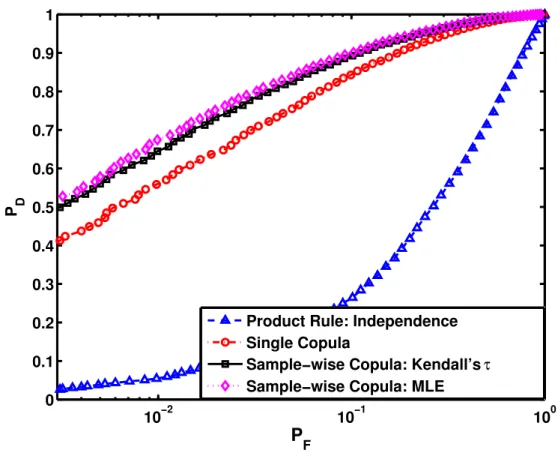
In Figures 2.1, 2.2 and 2.3 the receiver operating characteristics (ROC) curves are shown when different copulas were used to generate data. In Figure 2.1, we consider the case in which a single student’stcopula is used to generate the data. Note that this represents the case where the true copula is not known and is not included in the copula library. The label non-stationary copula refers to the sample-wise copula selection scheme proposed in this chapter. Figure 2.2 represents the case where half of allxnl were generated with a Gaussian copula and

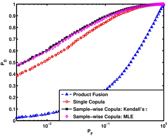
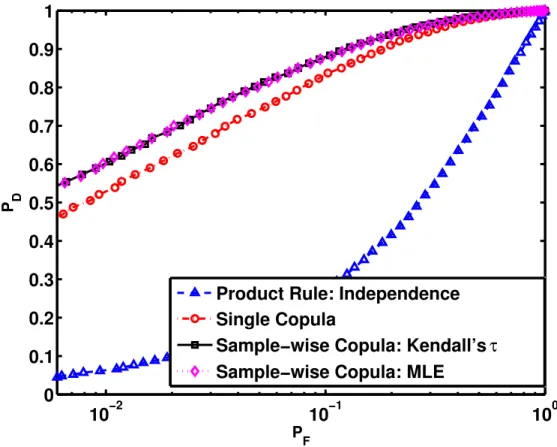
the remaining half consisted of samples generated from the Frank copula. This is, therefore, the case where the copula library contains both copula models that were used to generate data. The case of a single generating copula that is also a member of the library is also considered; Figure 2.3 shows results when all the data are generated using the Frank copula. It can be seen from Figures 2.1, 2.2 and 2.3 that for all three cases described above, our sample-wise selection rule outperforms the single copula rule, which has been theoretically justified in Proposition 2.1. All copula-based fusion rules which take inter-sensor dependence into consideration have better performance compared with the fusion rule under independence assumption.

For all simulation scenarios we observe that the GLRT and the test based onτˆ, using our selection scheme perform comparably. Both outperform the single copula selection method

(48)

10−2 10−1 100 0 0.1 0.2 0.3 0.4 0.5 0.6 0.7 0.8 0.9 P F P D

Product Rule: Independence Single Copula

Sample−wise Copula: Kendall’s τ

Sample−wise Copula: MLE

Fig. 2.1: ROCs forH1 data generated using atcopula

and product rules. We note that these results represent the unknown parameter case (Sec-tion 2.3.2), for which we were not able to prove that our method would outperform the single copula selection method. An intuition for why we observe this result is that sinceτˆ is con-sistent, for large L, τˆ → τ. Also, a single value of τ corresponds to different values of

φ_m = argcm(·), cm ∈ C. We conjecture that, asymptotically, this is as if the parameter

val-ues are known, allowing Proposition 2.1 to be applicable. This implies that whileτ controls theamountof dependence, which remains unchanged for allL, different copulas represent the

(49)

10−2 10−1 100 0 0.1 0.2 0.3 0.4 0.5 0.6 0.7 0.8 0.9 1 P F P D Product Fusion Single Copula

Fig. 2.2: ROCs forH1data generated using Frank and Gaussian copulas

2.5.2 Mixture of Copulas

In this subsection, we provide numerical results for the mixture of copula model for a two sensor case, i.e., N = 2. We assume normal and beta distributed marginals and consider the mixture of Gaussian and Gumbel, i.e.,C ={c1 =Gaussian, c2 =Gumbel}, with different

copula parameters. The marginals and the respective parameters used are tabulated in Table 2.1. We first investigate the performance of the EM algorithm in estimating copula parameters and the corresponding weights, i.e., Θ. When the samples are generated byc = 0.5c1(·|φ1 =

0.7) + 0.5c2(·|φ2 = 19), whose scatter plot is shown in Figure 2.4, The estimated Θ is as

follows: φˆ1 = 0.6879,πˆ1 = 0.5029; ˆφ2 = 19.3924,πˆ2 = 0.4971. From Figure 2.4, we can

visually distinguish the two different sets of samples generated by different copulas. The esti-mates are quite close to the true parameters in multiple trials.

(50)

10−2 10−1 100 0 0.1 0.2 0.3 0.4 0.5 0.6 0.7 0.8 0.9 P F P D

Product Rule: Independence Single Copula

Fig. 2.3: ROCs forH1 data generated using a Frank copula

When the samples are generated byc= 0.5c1(·|φ1 = 0.7) + 0.5c2(·|φ2 = 5), whose scatter

plot is shown in Figure 2.5, The estimatedΘis as follows: φˆ1 = 0.7243,πˆ1 = 0.5170; ˆφ2 =

4.5169,πˆ2 = 0.4830. In Figure 2.5, the two sets of samples are less distinguishable compared

with those in Figure 2.4. Also, the estimates vary from trial to trial.

When the samples are generated byc= 0.5c1(·|φ1 = 0.7) + 0.5c2(·|φ2 = 1.5), whose

scat-ter plot is shown in Figure 2.6, The estimatedΘis as follows:φˆ1 = 0.7230,πˆ1 = 0.4117; ˆφ2 =

1.5618,πˆ2 = 0.4117. In Figure 2.6, the two different sets of samples are hardly

distinguish-able. And the estimation results also show that the estimatedπ1 and π2 do not converge, and

their values are different from the true parameters.

In the EM algorithm, we use the convergence of log likelihood as the stopping criterion of the algorithm. Even though, the parameters may not converge to the true values, the log

(51)

0 0.1 0.2 0.3 0.4 0.5 0.6 0.7 0.8 0.9 1 0 0.1 0.2 0.3 0.4 0.5 0.6 0.7 0.8 0.9 1 F(x1) F(x 2 ) Gaussian copula (! 1=0.7) Gumbel copula(! 2=19)

Fig. 2.4: Scatter plot: mixture of Gaussian (φ1 = 0.7, π1 = 0.5) and Gumbel (φ2 = 19, π2 =

0.5) 0 0.1 0.2 0.3 0.4 0.5 0.6 0.7 0.8 0.9 1 0 0.1 0.2 0.3 0.4 0.5 0.6 0.7 0.8 0.9 1 F(x₁) F(x 2 ) Gaussian copula (φ1=0.7) Gumbel copula (φ2=5)

Fig. 2.5: Scatter plot: mixture of Gaussian (φ1 = 0.7, π1 = 0.5) and Gumbel (φ2 = 5, π2 =

0.5)

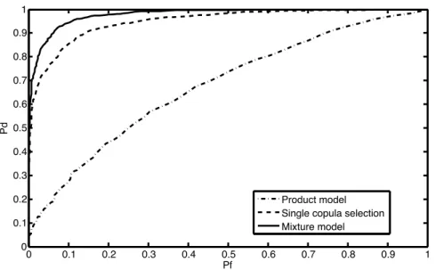
likelihoods converge to the ones that correspond to the true parameters. Since the Likelihood Ratio (LR) does not depend on the precision of these estimated parameters, but on the accuracy of the likelihood score, the detection performance of our approach is promising. We consider the case of data generated usingc = 0.5c1(·|φ1 = 0.7) + 0.5c2(·|φ2 = 1.5) as an example

to illustrate the detection performance of the mixture of copulas model. Figure 2.7 shows the ROCs for three different detection methods: mixture copula based detection, single copula based detection, and independent model. Using mixture of copulas model to describe the dependence structure underH1, results in a better detection performance compared with the

(52)

0 0.1 0.2 0.3 0.4 0.5 0.6 0.7 0.8 0.9 1 0 0.1 0.2 0.3 0.4 0.5 0.6 F(x₁) F(x 2 ) Gaussian copula (φ₁=0.7) Gumbel copula (φ₂=1.5)

Fig. 2.6: Scatter plot: mixture of Gaussian (φ1 = 0.7, π1 = 0.5) and Gumbel (φ2 = 1.5, π2 =

0.5)

single copula model and the independent model.

2.5.3 ARL Footstep Data

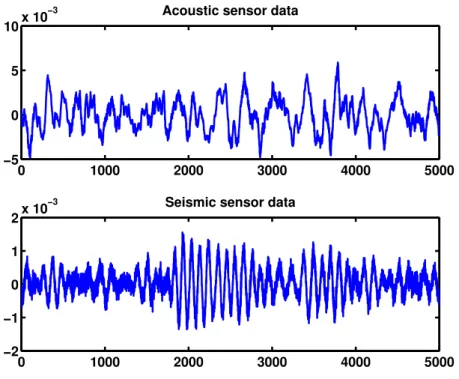
In order to test our proposed detection algorithms in the real world, we use the footstep data, made available by the US Army Research Laboratory (ARL), collected at Douglas, AZ to detect personnel activity. The dataset consists of raw observations from several sensors of different modalities that were deployed in an outdoor space to record human and animal activity that is typical in perimeter and border surveillance scenarios. The participants in the data collection exercise walked/ran along a predetermined path with sensors laid out along either side of the path. We consider copula-based seismic-acoustic fusion.

Seismic and acoustic time series for activities representing a single person walking (among other examples) are available in the ARL dataset. A representative dataset from acoustic and seismic sensors is shown in Figure 2.8. Each seismic/acoustic time series contains a leading 60s of background data. We use this as ourH0 data. The data are sampled at 10kHz, and are

mean centered and oscillatory in nature.

Before applying the copula-based detector, we first preprocess the data. The time series is split into non-overlapping frames of lengthT = 512. This raw time series data is calledxT n(t)

(53)

0 0.1 0.2 0.3 0.4 0.5 0.6 0.7 0.8 0.9 1 0 0.1 0.2 0.3 0.4 0.5 0.6 0.7 0.8 0.9 1 Pf Pd Product model Single copula selection Mixture model

Fig. 2.7: ROCs forH1data generated by the mixture of Gaussian and Gumbel.

wheren = 1,2 is the sensor index for the acoustic and seismic modalities respectively, and

t is the time index. In keeping with Houston’s analysis that Fourier spectra for seismic and acoustic footstep data are more informative than time-domain measurements [49], we set

xnl =

p

F {xT n(t)}2,

whereF is the DFT andl= 1, . . . , L= 256is the frequency index. Our sensor measurements are, therefore, now transformed to the frequency domain and the statistics ofx = [xnl] are

used as the input to the detector. The copula library consists of Gaussian, Gumbel and Frank copulas. We have observed that due to the interstitial nature of footstep data, including the independence copula in the library improves the overall detection performance.

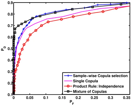
For the ARL dataset, the marginal distribution underH1, i.e.,fn(·|H1), n = 1,2, is

deter-mined non-parametrically anduij is obtained using the empirical probability integral transform

(EPIT). To generate ROCs, we compare the test-statistic to a vector of thresholds. The ROCs thus generated, for detectingH1 corresponding to one person walking againstH0