Development and Estimation of Traffic Data-Based Operational Measures for Effective Winter Snow Management
A THESIS
SUBMITTED TO THE FACULTY OF UNIVERSITY OF MINNESOTA
BY
Seong-Ah Hong
IN PARTIAL FULFILLMENT OF THE REQUIREMENTS FOR THE DEGREE OF
MASTER OF SCIENCE
Dr. Eil Kwon
ACKNOWLEDGEMENTS
I thank God for leading me through all my studies until this moment.
I would like to thank the Minnesota Department of Transportation (MnDOT) for sponsoring this project and providing the data.
I am indebted to a number of people without whom this project would not have been possible. First I appreciate my advisor, Dr. Eil Kwon, for providing me a platform to start the thesis project, for his incredible patience, rigorous challenges, his feedback and pertinent suggestions. I also appreciate the researchers in the NATSRL lab, Soobin Jeon and Dr. Chongmyung Park for their great contributions in developing the computer-based algorithm, and my undergraduate research assistant, Dowon Kim for always being out of his way to help me with.
Last but not least, I am grateful for my friends and family, who encouraged me continuously: My parents and inspiration, Minpyo Hong and Haksil Chang; my spiritual mentors, Isaiah Lee and Loisy Yoon who always supported me with the unfailing prays; my friends, Jinhong Lee, Myunghee Han, Jinju Lee, Sungji Hong and Sunghee Hong whom I love to be with forever in my life.
ABSTRACT
Snow storms degenerate safety and traffic mobility by creating adverse driving conditions including visibility impairments, reducing pavement friction, obstructed road facilities. Improving the effectiveness of the snow management requires an efficient assessment of the operational strategies with the data that can be directly measureable from the field. While there have been various types of operational measures used in the state DOTs in the US, the traffic data-based operational measures that can quantify the effects of snow plowing activities are still lacking. To be sure, the existing approaches developed to date employed the variations of traffic speed or travel time during the snow events and those measures cannot fully reflect the road weather conditions when traffic is congested.
Developing the operational measures that can objectively and accurately reflect the time-variant road weather conditions is essential in improving the effectiveness of the snow management strategies. In this research, an automatic process is developed for estimating the traffic data-based operational measures for winter snow management. Those measures include the Road Condition Recovery Time (RCR), the estimate of the ‘bare-lane regain time’, which is the major performance measure of the winter snow maintenance operations at the Minnesota Department of Transportation.
The automatic process was then applied to a sample snow section in Twin Cities, MN. The results of the example application showed that the operational measures can reasonably measure the performance of snow plowing operations by reflecting the impacts of the traffic flow resulted by the time-variant road weather conditions.
TABLE OF CONTENTS
ACKNOWLEDGEMENTS ... i
ABSTRACT ... ii
TABLE OF CONTENTS ... iii
LIST OF TABLES ... v LIST OF FIGURES ... vi CHAPTER 1: INTRODUCTION ... 1 1.1. Problem Statement ... 1 1.2. Research Objectives ... 2 1.3. Thesis Organization ... 3
CHAPTER 2: LITERATURE REVIEW ... 5
2.1. Existing Operational Measures for Winter Snow Management based on Traffic Data ... 5
2.2. Traffic Flow Behaviors under the Inclement Weather Conditions ... 8
2.2.1. Impacts of Weather Events on Traffic System ... 8
2.2.2. Traffic Flow Behaviors under the Inclement Weather Conditions ... 12
CHAPTER 3: COLLECTION OF TRAFFIC AND ROAD WEATHER DATA ... 15
3.1. Configuration of Snow Sections ... 15
3.2. Data Collection Process and Collected Data ... 19
3.2.1. Road Maintenance Information ... 21
3.2.2. Road Weather Information... 23
3.2.3. Traffic Flow Data ... 25
CHAPTER 4: ANALYSIS OF TRAFFIC FLOW PROCESS DURING SNOW EVENTS USING SECTION-WIDE FUNDAMENTAL DIAGRAMS ... 30
4.1. Development of Section-wide Fundamental Diagrams (SFD) for Snow Sections 30 4.2. Analysis of Section-wide Traffic Flow Process during Snow Events ... 33
4.2.1. Speed Variations Process during Snow Events ... 34
4.2.2. Traffic Flow Process during the Speed Reduction Period ... 37
4.2.3. Traffic Flow Process during Road Condition Recovery Period ... 41
4.2.4. Traffic Flow Process during Normal Traffic Pattern Recovery Period ... 55
4.3. Identification of Phase Change Points of Traffic Flow Process ... 59
4.3.1. Definitions of Phase Change Points ... 59
4.3.2. Characteristics of Phase Change Points ... 60
CHAPTER 5: DEVELOPMENT OF AUTOMATIC PROCESS FOR ESTIMATING OPERATIONAL MEASURES ... 65
5.2. Overview of the Automatic Process ... 70
5.3. Review of the Previous Studies and Enhancement on the Existing Process ... 77
5.3.1. Review of the Previous Studies ... 77
5.3.2. Enhancement on the Existing Process ... 79
5.4. Development of a Process for Identifying the Newly Identified Phase Change Points ... 86
5.4.1. Identification of WNR ... 86
5.4.2. Identification of RCR ... 97
5.4.3. Testing of RCR ... 117
5.5. Development of an Automatic Process for Estimating the Operational Measures ... 121
CHAPTER 6: EXAMPLE APPLICATION OF AUTOMATIC PROCESS WITH SAMPLE SNOW SECTION ... 124
6.1. Overview of Application Process ... 124
6.2. Example Estimation of Operational Measures for the Sample Snow Section ... 127
CHAPTER 7: CONCLUSIONS AND RECOMMENDATIONS ... 141
7.1. Summary of Findings ... 141
7.2. Limitations ... 145
7.3. Further Research Needs ... 146
LIST OF TABLES
Table 1: Base Value of Speed Reduction and SSI formula [3]... 6
Table 2: Information of the Selected Snow Corridor ... 18
Table 3: Road Weather Information of the Selected Snow Events ... 21
Table 4: Difference between the estimated RCR and the true RCR ... 118
Table 5: Distribution of the time difference between the estimated RCR and the “True RCR” ... 120
Table 6: Selected Snow Event Cases for the Example Application of Algorithm ... 130
Table 7: Example Result of the Operational Measures for the Snow Management within TH.94 for Each Snow Event ... 131
LIST OF FIGURES
Figure 1: Snow Route System in Twin Cities, MN, USA ... 16
Figure 2: (A) Configurations of Snow Routes; (B) Selected Snow Sections ... 18
Figure 3: Overall Process of Data Collection ... 20
Figure 4: CCTV images of Snow Plowing Trucks in Operations within a Section ... 24
Figure 5: Process to Calculate Section-wide Traffic Data ... 27
Figure 6: Smoothing Process using 3 minute Speed Variations ... 29
Figure 7: Section-wide Fundamental Diagrams of the Snow Section of 35E SB during Dry-Normal Day (December 13, 2012, 5:00-22:00) ... 31
Figure 8: Station Fundamental Diagrams of the Selected Stations within the Snow Section of 35E SB during Dry-Normal Day (December 13, 2012, 5:00-22:00) ... 32
Figure 9: Phase Change Points in Traffic Flow Variations of 94 EB Snow Section during snow events on January 14, 2012 (Normal: black / Snow: red) ... 35
Figure 10: Phase Change Points in Traffic Flow Variations of 94 EB Snow Section during snow events on January 20, 2012 ... 35
Figure 11: General Process of Snow-affected Speed Variations during Off-peak Time .. 36
Figure 12: General Process of Snow-affected Speed Variations during On-peak Time .. 36
Figure 13: Type 1 Reduction Pattern: Speed decreases with decreasing density ... 37
Figure 14: Type 2 Reduction Pattern: Speed decreases with increasing density ... 38
Figure 15: Type 3 Reduction Pattern: Speed decreases with sustaining density ... 39
Figure 16: Schematic Diagrams of the Reduction Pattern Types: Type 1 (Left); Type 2 (Middle); Type 3 (Right) ... 40
Figure 17: Snow plowing truck in Snow Section I-35E SB and the loop disturbance pattern in the SFD ... 42
Figure 18: Consecutive operations by snow plowing trucks in Snow Section I-35E SB and the two loop disturbance patterns in the SFD ... 42
Figure 19: Snow plowing truck in Snow Section 694 EB and the loop disturbance pattern in the SFD ... 43
Figure 20: Snow plowing truck in Snow Section 52 SB and the loop disturbance pattern in the SFD ... 43
Figure 21: Last loop pattern before reaching the posted limit appeared in the UK ... 44
Figure 22: Schematic Diagram of typical pattern of the counter-clockwise loop pattern 45 Figure 23: Impact of snow plowing operations under the insignificant traffic volumes within the section ... 45
Figure 24: Schematic Diagram of typical pattern of the clockwise loop pattern ... 47
Figure 25: Impact of snow plowing operations under significant traffic volume within the section ... 47
Figure 26: Road condition improvement due to Snow plowing operation executed on I-35E NB route. The density-disturbance pattern in SFD ... 48
Figure 27: Density-disturbance pattern appeared in UK plots before reaching the posted
speed limit... 49
Figure 28: Vertical increasing pattern appeared in UK plots before reaching the posted speed limit... 50
Figure 29: Distance weighted density values assigned for the segments ... 51
Figure 30: Two disturbance patterns identified in the SFD among which (B) were results of traffic flow variability (January 23. 2012 in I-94 WB Section) ... 52
Figure 31: Variations in the number of vehicles within a section where (B) involved a traffic volume variability ... 53
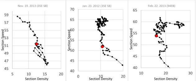
Figure 32: Selection of road condition recovery points before reaching the posted speed limit ... 54
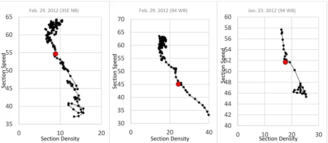
Figure 33: The wet normal recovery point in the SFD and speed variations when traffic flow recovered to the free-flow regime ... 56
Figure 34: The wet-normal recovery point in the SFD and speed variations when traffic flow recovered to the congested regime ... 57
Figure 35: Typical patterns of the Type 2 Recovery Pattern ... 57
Figure 36: Schematic Diagrams of Recovery Pattern Types: Type 1 (Left); Type 2 (Right) ... 58
Figure 37: Phase change points and the snow event information in the snow-affected speed variations ... 60
Figure 38: Determining RST Point in the Traffic Flow Variations of 94 WB Snow Corridor during snow events in January 14, 2012 ... 62
Figure 39: Phase change points and the snow event information in the snow-affected speed variations ... 66
Figure 40: Operational measures of time durations from SRST to the four different phase change points ... 68
Figure 41: Operational measures of time durations from the snow event end time to the three different phase change points ... 68
Figure 42: Operational measure of speed difference at LST compared to the dry-normal speed ... 69
Figure 43: Operational measure of ratio of snow-affected duration to the snow event duration ... 70
Figure 44: General Process of an Algorithm for Estimating the Operational Measures .. 71
Figure 45: Subordinate Process of Data Extraction and Processing ... 73
Figure 46: Subordinate Process of Identification of Phase Change Points ... 75
Figure 47: Subordinate Process of Estimation of Operational Measures ... 76
Figure 48: Identification of Phase Change Points of the Existing Algorithm [2] ... 78
Figure 49: Identification of Speed Recovery Point [2] ... 79
Figure 51: Flow Chart of Identification of RST ... 85
Figure 52: Flow Chart of Algorithm to Identify WNR ... 88
Figure 53: Flow Chart of Determination of Wet-Normal UK Curve ... 91
Figure 54: Selection of Reference Points and Testing Points in UK Diagram ... 93
Figure 55: Alteration of Testing Points with Consistent Reference Points ... 94
Figure 56: Alteration of Reference Points ... 95
Figure 57: Flow Chart of Identification of WNR ... 96
Figure 58: General Framework of Identification of RCR ... 98
Figure 59: Process of Determination of Range of RCR ... 99
Figure 60: Selection of Reference Points and Testing Points in UK Diagrams ... 101
Figure 61: Alteration of Testing Points with Consistent Reference Points ... 102
Figure 62: Alteration of Reference Points ... 102
Figure 63: Flow Chart of Identification of Loop-Disturbance Patterns ... 103
Figure 64: Traffic flow process of the K-disturbance pattern ... 104
Figure 65: Flow Chart of Identification of K-Disturbance Patterns ... 107
Figure 66: Traffic Flow Pattern of the Vertical-Increasing Pattern ... 108
Figure 67: Flow Chart of Identification of Vertical-Increasing Patterns ... 110
Figure 68: Flow Chart of Identification of Snow Plowing Patterns ... 113
Figure 69: Flow Chart of Identification of RCR ... 116
Figure 70: Distribution of the time difference between the estimated RCR and the “True RCR” ... 120
Figure 71: Subordinate Process of Estimation of Operational Measures ... 121
Figure 72: Editor Window for Route (Left) and Snow Event (Right) ... 125
Figure 73: Example Output of the Algorithm ... 126
Figure 74: Example Case of Graphical Output including the Speed Variation with Phase Change Points ... 127
Figure 75: Sample Snow Section within the TH.94 ... 128
Figure 76: Section-wide Flow-rate of Each Snow Section on the Jan. 14. 2012 ... 128
Figure 77: Section-wide Flow-rate of Each Snow Section on the Jan. 20. 2012 ... 129
Figure 78: Section-wide Flow-rate of Each Snow Section on the Jan. 23. 2012 ... 129
Figure 79: Section-wide Flow-rate of Each Snow Section on the Feb. 22. 2013 ... 129
Figure 80: Section-wide Flow-rate of Each Snow Section on the Mar. 18. 2013 ... 130
Figure 81: Estimation of Operational Measures for TH.94 EB in Jan. 14. 2012... 132
Figure 82: Estimation of Operational Measures for TH.94 WB in Jan. 14. 2012 ... 132
Figure 83: Estimation of Operational Measures for TH.94 EB in Jan. 20. 2012... 133
Figure 84: Estimation of Operational Measures for TH.94 WB in Jan. 20. 2012 ... 133
Figure 85: Estimation of Operational Measures for TH.94 EB in Jan. 23. 2012... 134
Figure 86: Estimation of Operational Measures for TH.94 WB in Jan. 23. 2012 ... 134
Figure 88: Estimation of Operational Measures for TH.94 WB in Feb. 22. 2013... 135 Figure 89: Estimation of Operational Measures for TH.94 EB in Mar. 18. 2013 ... 136 Figure 90: Estimation of Operational Measures for TH.94 WB in Mar. 18. 2013 ... 136 Figure 91: Maximum Speed Reduction vs. Average Road Surface Temperature (Left);
Maximum Speed Reduction vs. Average Daily Precipitation (Right) ... 138 Figure 92: Ratio of Snow-Affected Time vs. Average Road Surface Temperature (Left);
Ratio of Snow-Affected Time vs. Average Daily Precipitation (Right) ... 138
CHAPTER 1: INTRODUCTION 1.1. Problem Statement
It is important to accurately quantify and evaluate the performance of winter snow management during snow events. Well-conducted assessment on the current practices can obviate misusing the resources for the process of snow operations, such as: cost in operating the snow plowing trucks, number of people assigned to snow duty, and tons of materials used. Also, it can improve the effectiveness of the operational process to result in the better output, such as: reduction of travel time delay, improvements in traffic-flow level of service, and decrease in crash rates.
Currently, the most of state DOTs including the Minnesota Department of Transportation (MnDOT) use the “Time to bare pavement” for winter snow operations [1]. The “Time to bare pavement” is defined as the duration from the snow event end time to the “bare lane regain time.”
MnDOT defines the bare lane regain conditions as having all driving lanes free of snow and ice between the outer edges of the wheel paths and having less than 1 inch of accumulation on the center of the roadway. It is regarded such conditions indicate that drivers become feel safe to drive with a posted speed limit if traffic is not congested.
Practically, however, the “bare lane regain time” for the snow event is determined by the visual inspections of the field crews involved in the snow plowing operations. Such methodology of determining the “bare lane regain time” possibly imposes the issues of objectivity and accuracy to be compliance with the standards of DOT’s.
While, it is evident that the road weather conditions affects the traffic flow behaviors during snow events as substantiated by many researchers. However, the efforts to use the traffic data in determining the operational measure such as the “bare lane regain time” has not been a common practice yet.
The research group at the University of Minnesota Duluth has developed an algorithm to estimate the “Speed Recovery Time” to estimate the “bare lane regain time” using the speed variations during snow events [2]. However, it has been noted that only the inspection of speed variations were not sufficient to make a decision pertaining to “the bare lane regain time,” as the speed variations are affected by both snow and traffic congestion. With those limitations, it was called for developing alternative measurements which can represent the current conditions of traffic flow which is reliable to the traffic congestions, such as the process of a relationship between the two parameters of traffic flow.
1.2. Research Objectives
The goal of this research in to develop an automatic process for estimating the alternative traffic data-based operational measures for winter snow management. The automatic process will be applied to the metro freeways in the Twin Cities, Minnesota, with the winter snow event data in 2012-2013.
1) Identification of phase change points within the traffic flow process including the “road condition recovery time” which can be a surrogate for the “bare lane regain time.”
2) Development of traffic data-based operational measures using the phase change points defined in the study.
3) Development of an automatic process for estimating the operational measures for winter snow management and operations.
1.3. Thesis Organization
The remaining chapters of this thesis were organized as follows:
Chapter 2 presents a relevant literature review on the following subjects: 1) Existing research efforts on the operational measures for winter snow management, and 2) Effects of the weather conditions on the traffic flow behaviors.
Chapter 3 describes the dataset used in this study. The data collection process and the summary of the collected will be provided.
Chapter 4 presents the analysis of the snow-affected traffic flow process using the section-wide speed variations and the Section-wide Fundamental Diagrams (SFD). Based on the result of analysis, a set of phase change points was identified in the traffic flow variations.
Chapter 5 describes the automatic process for estimating the operational measures for winter snow management. First, a set of the alternative operational measures based on
traffic data will be developed using the phase change points identified in the previous chapter. Then, the step-by-step process of the algorithm developed in this study will be presented.
Chapter 6 demonstrates the applications of the automatic process to the sample snow section. The results of estimation of the alternative operational measures for the given snow event cases will be provided and interpreted.
Chapter 7 summarizes the research efforts, key findings, conclusions, and recommendations for future research.
CHAPTER 2: LITERATURE REVIEW
In Chapter 2, the relevant literatures and the up-do-date practices of operational measures for winter snow management will be reviewed. The following subjects will be covered:
2.1 Existing Operational Measures for Winter Snow Management based on Traffic Data
2.2 Existing Studies on Traffic Flow Behaviors under the Inclement Weather Conditions
2.1. Existing Operational Measures for Winter Snow Management based on Traffic Data
Iowa Department of Transportation
Iowa Department of Transportation estimates the acceptable speed reduction during a storm as in
Equation 1 [3]:
Acceptable Speed Reduction = BVSR × SSI
Equation 1 In Equation 1, BVSR (Base Value of Speed Reduction) indicates the maximum acceptable speed reduction for a given route under the worst storm. SSI (Storm Severity
Index) refers the severity level of a storm which is determined by the different elements of the snow storm, such as the storm type, storm temperature, wind conditions and its behavior characteristics. Table 1 provides the values of BVSR (Base Value of Speed Reduction) for different route categories in terms of their priorities. Also, the table summarizes the set of index values which will be used in determining the SSI for a certain conditions of a snow storm. The formula to calculate SSI is provided in Equation 2:
𝑆𝑆𝐼 = [1
𝑏× [𝑆𝑇 × 𝑇𝑖 × 𝑊𝑖 + 𝐵𝑖 + 𝑇𝑝+ 𝑊𝑝− 𝑎]]
0.5
where 𝑎 = 0.0005 and 𝑏 = 1.6995
Equation 2 The success of the performance of winter snow management will be determined by comparing the measured speed drop to the “Acceptable Speed Reduction” resulted by the above process.
Table 1: Base Value of Speed Reduction and SSI formula [3] Base Value of Speed Reduction
(mph)
Priority A Priority B Priority C
17 22 24
Storm Type (ST) Freezing Rain 0.72 Light Snow 0.35 Medium Snow 0.52 Heavy Snow 1 Storm Temperature (𝑇𝑖) Warm 0.25 Medium Range 0.4 Cold 1
Wind Conditions in Storm (𝑊𝑖) Light 1 Strong 1.2
Early Storm Behavior (𝐵𝑖) Starts as Snow 0 Starts as Rain 0.1
Post Storm Temperature (𝑇𝑝) Same 0 Warming -0.087 Cooling 0.15
University of Wisconsin at Madison [4]
In an attempt to develop the traffic data-based operational measure for quantifying the performance of winter snow management, the regression model to estimate the “speed recovery duration” was formulated as a function of several variables including the maximum speed reduction (%), time to maximum speed reduction, and snow depth due to a given snow storm, as in Equation 4, using the traffic data collected from the Madison, Wisconsin:
Speed Recovery Duration =
9.68 + 9.926×MSRPCENT – 0.086×StoS2MSR + 0.493×Crewdelayed – 0.222×Snowdepth
Equation 3 where,
MSR = Maximum speed reduction,
StoS2SD = Time lag to speed drop after snow storm starts StoS2MSR = Time to MSR after snow storm starts
Crewdelayed = Time lag to deploy maintenance crew after snow storm starts Snowdepth = Snow precipitation
While their effort needs to be recognized as one of the first ones in applying traffic-flow data for quantifying the performance of snow operations, Kwon [2] pointed out that the method of piecewise linear regression resulted in the questionable models, e.g., negative parameter of the “Snowdepth” variable.
Michigan Department of Transportation [5]
Michigan Department of Transportation adopted the traffic data –based performance measure called “Weather Travel Impacts.” The measure determines the success of the snow operational measures by the fact whether the normal speeds were regained within two hours or less, 80% of the time for winter weather events. To develop the normal speeds to be used as a reference, MDOT collected the speed data along I-96, from Ionia County to the Oakland County line during the winters of 2009-2012. The portable trailers with microwave sensors were attached to detect speed before, during and after a winter storm event. Also, storm start and end times are recorded by maintenance staff along with other information about the intensity and temperatures during the storm.
Even though such effort to use the traffic data in estimating the performance of the winter snow operations has to be recognized, only employing the speed variations in determining the road recovery time has a limitation in the case of traffic congestion.
2.2. Traffic Flow Behaviors under the Inclement Weather Conditions
2.2.1.Impacts of Weather Events on Traffic System
Weather events including rain, snow and fog build up inclement driving conditions which are different from dry normal condition. The inclement conditions describe visibility impairments, reducing pavement friction, obstructed road facilities, restricted vehicle performance, etc. Depending on weather type, duration, and intensity, the scenarios of roadway condition may vary and that impacts on transportation system also differ.
Typically, the influences of the inclement weather on the transportation system can be examined in three parts: safety, traffic flow, and operational productivity.
Safety
The environment with lowered visibility and slippery pavement can result in the increase in frequencies and severities of crashes. According to the crash data collected in the US in 1995-2008, the weather-related crashes were reported greater than 1.5 million vehicle crashes per year while comprising 24% of the whole population of crash incidents each year [6]. Among the weather-related accidents, the significant majority of crashes happened on wet pavement and during rainfall, reporting 75% and 45% of the entire weather-related crashes respectively. While, small amount of crashes occurred during winter snow conditions; amount of crashes in snow or sleet condition involved 15% and those on icy pavements accounted for 13% of weather-related incidents [6]. This result reflects the tendency of drivers who became more cautious during snow event than rainfall. While, the study efforts to identify the impacts of weather events on the severity of crash were also conducted. It was observed that 17% of the entire crash fatalities was attributed to the weather events, which implies that the weather condition also aggravate severity of crashes as well as the increase in the number of amount [6]. A similar study was conducted in Canada [7]. They disclosed that snow days had fewer fatal crashes than dry days, but more nonfatal-injury crashes and property-damage-only crashes were reported [7]. The study also showed that the first snow day of the year was substantially more dangerous
than other snow days in terms of fatalities, particularly for elderly drivers [7]. Some comparable observations with the previous study relating to the behavior of motorists under snow events were also observed in the study in the US [8].
Traffic Flow and Mobility
The nation-wide efforts to measure and quantify the influences of inclement weather on traffic flow have been conducted using the empirical or simulated data. Ibrahim et al. [9] identified the impact of inclement weather on traffic speed by differentiating the types (rain and snow) and intensity (light and heavy) of precipitation. It was observed the minimal reductions in the operating speeds in light rain, but significant reductions in heavy rain: in light rain, a 2.0 km/h (1.7%) reduction in speed during free-flow conditions was found typical; in heavy rain, a 5.0-10.0 km/h (4.4-8.7%) reduction in free-flow speed was estimated [9]. Likewise, light snow was found to have minimal effects on speed but heavy snow imposes potentially large effects on operating speeds. Light snow resulted in a statistically significant drop of 0.96 km/h in free-flow speeds. Heavy snow resulted in a 38.0 - 50.0 km/h free-flow speed reduction (33- 43%) [9]. More recent study by Rakha et al. provides consistent findings for major traffic flow parameters: the light rain (0.01 cm/h) results in reductions in the traffic stream free flow speed, speed at capacity, and capacity in the range of 2-3.6%, 8-10%, and 10-11%, respectively [10]. Also, light snow (0.01cm/h) produces reductions in free flow speed, speed at capacity, and capacity in the range of 5-16%, 5-5-16%, and 12-20%, respectively [10]. They concluded that the reductions in the free
flow speed and the speed at capacity both increased under the greater intensity of rain or snow. While, traffic jam density and roadway capacity reduction remain constant for all weather intensities at a specific site [10].
Operational Productivity of Traffic System
The inclement weather conditions also deteriorate operational productivity of transportation system while increasing the cost of operating and maintenance of winter road maintenance, traffic management, emergency management, and law enforcement. According to FHWA data collected in 1997-2005, winter road maintenance accounted for roughly 20% of state DOT maintenance budgets and that state and local agencies spend more than 2.3 billion dollars on snow and ice control operations annually [11]. In addition, trucking companies and commercial vehicle operators lose an estimated 32.6 billion vehicle hours due to weather-related congestion in 281 of the nation's metropolitan areas each year [12]. Nearly 12% of total estimated truck delay is due to weather events in the 20 cities with the greatest volume of truck traffic [12]. The estimated cost of weather-related delay to truck companies ranges from 2.2 - 3.5 billion dollars annually [12].
All these studies show that inclement weather may have a significant and comprehensive impact on the transportation system, which cannot be ignored by planners and decision makers.
2.2.2.Traffic Flow Behaviors under the Inclement Weather Conditions
To effectively mitigate the adverse impacts of the inclement weather on traffic system, FHWA has involved researchers and universities in the US and abroad to tackle an organized research framework upon Weather Responsive Traffic Management (WRTM) [13]. The WRTM research projects include: collecting and analyzing data, developing models and tools to improve the analysis, and modeling/prediction of traffic flow in all types of weather conditions. In a project completed in 2008 by Rakha et al., the impacts of inclement weather on traffic were quantified by developing Weather Adjustment Factors (WAF) for key traffic flow parameters (e.g., the free flow speed, speed at capacity, capacity, and jam density) [10]. The WAF for each traffic parameter was estimated by developing multiple linear regression model using precipitation type, precipitation intensity, and visibility level as independent variables. This study made a contribution to form fundamental basis for developing WRTM strategies. For example, the WAF can be implemented in the HCM freeway procedures by multiplying the base clear-condition factors by the WAFs. The potential applications of WAFs on the WRTM strategies include: (1) the capacity values that are used for the design of roadways could be modified to reflect the impact the impact of precipitation. (2) the procedures could be incorporated in real time advanced traffic management system applications, namely, ramp metering or adaptive signal control algorithms. This refinements in traffic control devices provides better estimates of roadway capacity and thus enhance these real-time systems [10]. In addition, researchers already incorporated such results in analyses using traffic simulation modeling
tools, such as DYNASMART, DynaMIT, AIMSUN, CORSIM, INTEGRATION, PARAMICS, VISSIM and others [13].
Moving from macro to micro analysis, FHWA looked at individual driver responses to weather conditions, such maneuvers as: changing lanes, merging onto a freeway, making a left turn across traffic at an intersection, and adjusting the distance behind a lead vehicle. Using video data from intersections in Virginia and test tracks in Japan, the manner by which drivers perceive and accept gaps in traffic streams were analyzed and used to develop relationships that can support traffic signal phasing adjustments during weather events [14]. Notwithstanding the progress in the study on the microscopic traffic flow behavior during weather conditions, this area remains to have limitations and erroneous future work is expected to illuminate the process of data collection and integration and theoretical analysis of driver behavior in adverse weather. In addition, modeling of headway distribution that considers vehicle class, vehicle type, time of the day, and day of the week could benefit a process of determining traffic stability.
The goal of the above studies within the WRTM framework is to inform model development and decision-support tools to allow a user to translate current and forecast conditions to traffic impacts. In addition to the macroscopic and microscopic traffic flow research, the FHWA RWMP modified two Traffic Estimation and Prediction System (TrEPS) tools to account for weather impacts and improve their traffic estimation and prediction capabilities and overall utility [15]. Those models of TrEPS are
DYNASMART-P, a system for transportation planning, and DYNASMART-X, a real-time system for predicting traffic conditions and patterns [13].
Based on the literature reviews on the weather impact on the traffic flow, one of the main issues with the existing approaches was that most of the studies assumed that the amount of impacts on traffic flow sustained equal within a weather event. In reality, however, the road weather conditions show a wide ranges of variations through a single weather event, causing the traffic flow responds in a different ways to the dynamically changing environments. This issue has prevented the results from being used in any practical purposes, such as the development of the traffic data-based operational measures of winter snow operations. To resolve this issue, it is needed to study the temporal process of traffic flow with the connection of the varying road weather conditions during snow events.
CHAPTER 3: COLLECTION OF TRAFFIC AND ROAD WEATHER DATA
In Chapter 3, the study area and dataset used for the research will be described using the following terms:
3.1. Configuration of Snow Sections
3.2. Data Collection Process and Collected Data
The study area is comprised of selected “snow sections” which will be identified and defined in Chapter 3.1. The dataset for the study includes three types: road maintenance data, road weather data and traffic flow data. The procedure for processing each type of data will be explained further in Chapter 3.2.
3.1. Configuration of Snow Sections
The overall scheme of winter snow management and operations are planned, executed and evaluated within the framework of the snow route system. Currently, the snow route system is made up of the primary freeways in the vicinity of the metropolitan network in Twin Cities, Minnesota. Figure 1 includes a map of the snow route system which was provided by the Office of Maintenance Operations of the Minnesota Department of Transportation (MnDOT). The snow route system consists of 75 snow routes and each individual snow route is identified by the different colored threads on the map. Under the MnDOT’s policy, snow routes in close proximity were grouped to be assigned to a truck station for the control of snow management and operations for the given snow routes. It
should be noted that the snow route system in the metropolitan area is associated with 18 truck stations across the region.
(http://www.dot.state.mn.us/maintenance/pdf/research/manual/Ch1.pdf)
Figure 1: Snow Route System in Twin Cities, MN, USA
According to the practices of the MnDOT, snow plowing operations and performance evaluations are independently conducted for each individual snow route. The bare lane regain time, the main performance measure used by the MnDOT, is reported based on the snow route system, which means that one snow route is assigned with one specific bare lane regain time.
However, one separate snow route consists of multiple segments of different highways. Figure 2 (A) shows the two selected snow routes which are located in the central area of the Twin Cities. The identification numbers of the snow routes include TP9F0251
and TP9F0253 under the MnDOT Snow Route Identification System. As shown in the figure, Snow Route TP9F0251 is comprised of two segments of different freeways (i.e., I-35E and TH.694) and thus Snow Route TP9F0253 (i.e., I-94 and TH.52) is done in a similar fashion.
In this study, such types of snow routes were divided into two different components called “snow sections” which are made up of a consistent freeway. For example, as appears in Figure 2 (B), Snow Route TP9F0251 was divided into two snow sections which include the freeway segment of I-35E and TH.694, respectively. In a similar fashion, Snow Route TP9F0253 was divided into two snow sections that include freeway segments I-94 and TH.52, respectively. It should also be noted that the boundaries of snow sections were designed in a way that the traffic flow can maintain consistent characteristics across the snow section without significant interruptions incurred by the traffic flow entering and exiting through the ramps connected to the various freeways. In this study, the four snow sections shown in Figure 2 (B) will be utilized.
Figure 2: (A) Configurations of Snow Routes; (B) Selected Snow Sections
As shown in Table 2, the length of each of the selected snow sections is usually within 5 miles, which takes less than 5 minutes for road users to drive through under free-flow conditions. It allows the traffic data collected from the different stations within a section to be reasonably aggregated to reflect the global features of the section-wide traffic flow.
Table 2: Information of the Selected Snow Corridor
Snow
Corridor Length (miles) Posted Speed Limit (mph)
Estimated Travel Time under the Posted Speed
Limit (min) I-35E 4.9 60 4.9 T.H. 694 4.5 60 4.5 I-94 4.7 55 5.1 T.H. 52 1.1 55 1.2 (A) (B)
3.2. Data Collection Process and Collected Data
An overview of the dataset used in this study is shown in Figure 3 below. It consists of three types which include road maintenance/operations information, road weather information and traffic flow data.
As for the road maintenance/operations dataset, it was compiled from the PPMS report (Program and Project Management System) provided by the MnDOT. The two main types of data used in the PPMS report were the snow event start/end time and the reported bare lane regain time. Using that information, the list of snow events for this research was determined and the approximate road condition recovery time was established.
In terms of road weather condition data, it was collected from two different sources, including the MnDOT Traveler Information website and the Road Weather Information System (RWIS). Through the MnDOT Traveler Information website, CCTV images displaying real-time road conditions during snow events were collected to record significant improvements in road conditions and to capture any moments where snow plowing operations were executed within a section. This data was used to identify any traffic flow patterns during the times of individual plowing operation.
Another source of road weather data was the RWIS. Among the RWIS dataset, the daily database on the precipitation type and the variations of precipitation were accessed to identify the normal days within a predetermined period. The list of the selected dry-normal days was employed to develop a dry-dry-normal pattern which was used in the
comparative analysis between snow-affected traffic patterns and dry-normal traffic patterns.
Lastly, a traffic flow dataset was collected from inductive loop detectors installed on the Metropolitan freeways in the Twin Cities. Primitive types of data in the form of vehicle counts and occupancy rates were processed to macroscopic traffic flow parameters such as flow rate, density and speed. Using those parameters, traffic patterns during both dry-normal days and snow events were developed to identify the features of snow-affected traffic flow processes during snow events. The details on the collection process for each type of data will be described in the sections to follow.
Road Maintenance
Information Road Weather Information Traffic Data
Data Source Data Source Data Source Data Source
MnDOT Program and Project Management System (PPMS) MnDOT Traveler Information Road Weather Information System (RWIS) Traffic Management Center Server
Data Type Data Type Data Type Data Type
Snow event start/end time, Bare lane regain time
CCTV images
Road surface condition, Accumulative
precipitation
Loop detector data (vehicle counts and occupancy rate)
↓ ↓ ↓ ↓
Information on the snow events
Approximate time of bare lane
regain time
Identification of the time of snow plowing operations
Selection of the normal dry days
Development of traffic flow patterns
3.2.1.Road Maintenance Information
The PPMS reports (Program and Project Management System) provided by the MnDOT include information regarding snow events and snow plowing operations as listed below. It needs to be noted that the lane regain time occurs in 30 minute increments.
Snow Weather Information: Plow route, Weather condition, Snow event start time, Snow
event end time, and Snow event duration
Snow Plowing Operations Information: Lane lost time, Bare lane regain time, Lane lost
duration, and Recovery hours
In Table 3, 56 cases of snow events for different snow sections were selected for this research among snow events taking place between November 2011 and March 2013. Table 3: Road Weather Information of the Selected Snow Events
Snow
Route Freeway Corridor Snow Event Start Time Snow Event End Time Lane Regain Time
TP9F0251
I-35E NB
11/19/2011(Sat) 11:00 11/19/2011(Sat) 18:30 11/19/2011(Sat) 17:30
1/14/2012 (Sat) 10:00 1/14/2012 (Sat) 18:10 1/14/2012 (Sat) 17:00
1/20/2012 (Fri) 6:15 1/20/2012 (Fri) 13:45 1/20/2012 (Fri) 13:15
1/23/2012 (Mon) 1:30 1/23/2012 (Mon) 10:30 1/23/2012 (Mon) 11:00
2/28/2012 (Tue) 7:20 2/29/2012 (Wed) 10:15 2/29/2012 (Wed) 9:09
2/22/2013 (Fri) 1:00 2/22/2013 (Fri) 11:15 2/22/2013 (Fri) 10:30
3/14/2013 (Thu) 3:45 3/14/2013 (Thu) 9:00 3/14/2013 (Thu) 9:30
3/18/2013 (Mon) 4:30 3/18/2013 (Mon) 17:00 3/18/2013 (Mon) 12:00
I-35 SB
11/19/2011(Sat) 11:00 11/19/2011(Sat) 18:30 11/19/2011(Sat) 17:30
1/14/2012 (Sat) 10:00 1/14/2012 (Sat) 18:10 1/14/2012 (Sat) 17:00
1/20/2012 (Fri) 6:15 1/20/2012 (Fri) 13:45 1/20/2012 (Fri) 13:15
1/23/2012 (Mon) 1:30 1/23/2012 (Mon) 10:30 1/23/2012 (Mon) 11:00
2/28/2012 (Tue) 7:20 2/29/2012 (Wed) 10:15 2/29/2012 (Wed) 9:09
2/22/2013 (Fri) 1:00 2/22/2013 (Fri) 11:15 2/22/2013 (Fri) 10:30
3/14/2013 (Thu) 3:45 3/14/2013 (Thu) 9:00 3/14/2013 (Thu) 9:30
3/18/2013 (Mon) 4:30 3/18/2013 (Mon) 17:00 3/18/2013 (Mon) 12:00
TH.694 EB
1/14/2012 (Sat) 10:00 1/14/2012 (Sat) 18:10 1/14/2012 (Sat) 17:00
1/20/2012 (Fri) 6:15 1/20/2012 (Fri) 13:45 1/20/2012 (Fri) 13:15
1/23/2012 (Mon) 1:30 1/23/2012 (Mon) 10:30 1/23/2012 (Mon) 11:00
2/28/2012 (Tue) 7:20 2/29/2012 (Wed) 10:15 2/29/2012 (Wed) 9:09
2/22/2013 (Fri) 1:00 2/22/2013 (Fri) 11:15 2/22/2013 (Fri) 10:30
3/14/2013 (Thu) 3:45 3/14/2013 (Thu) 9:00 3/14/2013 (Thu) 9:30
3/18/2013 (Mon) 4:30 3/18/2013 (Mon) 17:00 3/18/2013 (Mon) 12:00
TH.694 WB
11/19/2011(Sat) 11:00 11/19/2011(Sat) 18:30 11/19/2011(Sat) 17:30
1/14/2012 (Sat) 10:00 1/14/2012 (Sat) 18:10 1/14/2012 (Sat) 17:00
1/20/2012 (Fri) 6:15 1/20/2012 (Fri) 13:45 1/20/2012 (Fri) 13:15
1/23/2012 (Mon) 1:30 1/23/2012 (Mon) 10:30 1/23/2012 (Mon) 11:00
2/28/2012 (Tue) 7:20 2/29/2012 (Wed) 10:15 2/29/2012 (Wed) 9:09
2/22/2013 (Fri) 1:00 2/22/2013 (Fri) 11:15 2/22/2013 (Fri) 10:30
3/14/2013 (Thu) 3:45 3/14/2013 (Thu) 9:00 3/14/2013 (Thu) 9:30
3/18/2013 (Mon) 4:30 3/18/2013 (Mon) 17:00 3/18/2013 (Mon) 12:00
TP9F0253
I-94 EB
1/14/2012 (Sat) 10:15 1/14/2012 (Sat) 18:25 1/14/2012 (Sat) 21:30
1/20/2012 (Fri) 6:15 1/20/2012 (Fri) 13:45 1/20/2012 (Fri) 13:15
1/23/2012 (Mon) 1:30 1/23/2012 (Mon) 10:30 1/23/2012 (Mon) 11:00
2/28/2012 (Tue) 7:20 2/29/2012 (Wed) 10:15 2/29/2012 (Wed) 9:09
2/22/2013 (Fri) 1:00 2/22/2013 (Fri) 10:15 2/22/2013 (Fri) 11:00
3/18/2013 (Mon) 4:30 3/18/2013 (Mon) 17:00 3/18/2013 (Mon) 10:00
I-94 WB
1/14/2012 (Sat) 10:15 1/14/2012 (Sat) 18:25 1/14/2012 (Sat) 21:30
1/20/2012 (Fri) 6:15 1/20/2012 (Fri) 13:45 1/20/2012 (Fri) 13:15
1/23/2012 (Mon) 1:30 1/23/2012 (Mon) 10:30 1/23/2012 (Mon) 11:00
2/28/2012 (Tue) 7:20 2/29/2012 (Wed) 10:15 2/29/2012 (Wed) 9:09
2/22/2013 (Fri) 1:00 2/22/2013 (Fri) 10:15 2/22/2013 (Fri) 11:00
3/18/2013 (Mon) 4:30 3/18/2013 (Mon) 17:00 3/18/2013 (Mon) 10:00
TH.52 NB
1/14/2012 (Sat) 10:15 1/14/2012 (Sat) 18:25 1/14/2012 (Sat) 21:30
1/20/2012 (Fri) 6:15 1/20/2012 (Fri) 13:45 1/20/2012 (Fri) 13:15
1/23/2012 (Mon) 1:30 1/23/2012 (Mon) 10:30 1/23/2012 (Mon) 11:00
2/28/2012 (Tue) 7:20 2/29/2012 (Wed) 10:15 2/29/2012 (Wed) 9:09
2/22/2013 (Fri) 1:00 2/22/2013 (Fri) 10:15 2/22/2013 (Fri) 11:00
3/18/2013 (Mon) 4:30 3/18/2013 (Mon) 17:00 3/18/2013 (Mon) 10:00
TH.52 SB
1/14/2012 (Sat) 10:15 1/14/2012 (Sat) 18:25 1/14/2012 (Sat) 21:30
1/20/2012 (Fri) 6:15 1/20/2012 (Fri) 13:45 1/20/2012 (Fri) 13:15
1/23/2012 (Mon) 1:30 1/23/2012 (Mon) 10:30 1/23/2012 (Mon) 11:00
2/28/2012 (Tue) 7:20 2/29/2012 (Wed) 10:15 2/29/2012 (Wed) 9:09
2/22/2013 (Fri) 1:00 2/22/2013 (Fri) 10:15 2/22/2013 (Fri) 11:00
3.2.2.Road Weather Information
RWIS data (http://rwis.dot.state.mn.us/)
RWIS (Road Weather Information System), committed to most of the state DOTs in the United States, is a central communication system that aims to transfer and collect field data from numerous Environmental Sensor Stations (ESS). ESS is the principal base station of weather data collection and the collected data includes both atmospheric and pavement data. Atmospheric data includes air temperature and humidity, visibility distance, wind speed and direction, precipitation type and rate, etc. Pavement data includes pavement temperature, pavement freezing point, pavement conditions (e.g., wet, icy, flooded), surface conditions, etc. It should be noted that the pavement data is primarily unique in nature and highly site-specific. Central RWIS hardware and software are used to process the observations from ESS to develop real-time casting or forecasts and disseminate road weather information in a format that can be easily interpreted by users.
In this study, daily precipitation data through all months was inspected within the same month of the snow event to select all possible “dry-normal days.” The “dry-normal day” was defined as one where the precipitation remains zero and the road surface conditions continue to be dry all day. The selected dry-normal days were used to develop an average dry-normal pattern for each snow event, which was subsequently used to identify the impact of weather events on traffic flow variations and to determine the phase change points in traffic variations.
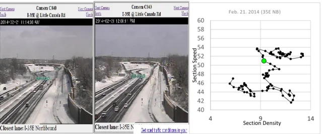
CCTV (Closed-Circuit Television) Images
The real-time CCTV images were collected from the MnDOT Traveler’s Information website for the selected snow sections during snow events from December 2013 to February 2014. Data was collected every 15 to 30 minutes when snow plowing operations were actively executed. However, there were some difficulties in data collection as it was only possible to manually clip an image of one spot at a time to proceed through the entire study areas in sequence. As shown in Figure 4, it was identified when snow plowing trucks were deployed and/or the significant improvements in the road conditions were made. Such information supported the analysis of traffic flow patterns at the road condition recovery periods.
3.2.3.Traffic Flow Data
Station Traffic Flow Data
Inductive loop detectors are located on the mainline of freeways approximately every half mile and on entrance and exit ramps. The loop detectors collect information about vehicle counts and occupancy rates and report the data back to the Traffic Management Center (TMC) every 30 seconds.
That primitive form of data was accessed using the TICAS (Traffic Information and Condition Analysis System), developed at University of Minnesota Duluth to estimate the macroscopic parameters of traffic flow, e.g., flow rate (q), speed (u) and density (k). The traffic flow parameters were estimated based on the equations seen below. Then, traffic data in 30-second intervals were aggregated into 3-minute intervals to reduce the random fluctuations on the traffic patterns.
𝑞 (𝑣𝑒ℎ/ℎ𝑟) =𝑣𝑒ℎ𝑖𝑐𝑙𝑒 𝑐𝑜𝑢𝑛𝑡𝑠 (𝑣𝑒ℎ) 30 𝑠𝑒𝑐 (3600 𝑠𝑒𝑐1ℎ𝑟 ) Equation 4 𝑘 (𝑣𝑒ℎ/𝑚𝑖) =5280 × 𝑂𝑐𝑐𝑢𝑝𝑎𝑛𝑐𝑦 (%) 𝐿 (𝑓𝑡) + 𝐿𝐷 (𝑓𝑡) Equation 5 𝑢 (𝑚𝑝ℎ) = 𝑓𝑙𝑜𝑤 𝑟𝑎𝑡𝑒 (𝑣𝑒ℎ/ℎ𝑟) 𝑑𝑒𝑛𝑠𝑖𝑡𝑦 (𝑣𝑒ℎ/𝑚𝑖) Equation 6 where,
𝐿 = Average Vehicle Length (ft)
Section-wide Traffic Flow Data
The station-based traffic flow data was then processed to develop a section-wide averaged data weighed by distance. The process to estimate the section-wide traffic flow parameters is demonstrated in the schematic diagram in Figure 5. The section includes the three stations, i.e., Station 1-3, of which the traffic flow parameters at time t are denoted as
𝑞𝑖,𝑡, 𝑘𝑖,𝑡 and 𝑢𝑖,𝑡 when i refers to the station number. For example, Station 1 involves
𝑞1,𝑡, 𝑘1,𝑡 and 𝑢1,𝑡, Station 2 involves 𝑞2,𝑡, 𝑘2,𝑡 and 𝑢2,𝑡, and Station 3 involves 𝑞3,𝑡, 𝑘3,𝑡 and
𝑢3,𝑡 at time t.
The distance between Station i and Station i+1 was indicated as 𝐿𝑖. For instance, 𝐿1
refers to the distance between Station 1 and 2, and 𝐿2 refers to the distance between Station 2 and Station 3. As appears in the figure, each 𝐿𝑖 was evenly divided into three segments to be allocated with different values of traffic data. For example, the left-end segment located near Station 1 was assigned with 𝑞1,𝑡, 𝑘1,𝑡 and 𝑢1,𝑡, and the right-end segment located near Station 2 was assigned with 𝑞2,𝑡, 𝑘2,𝑡 and 𝑢2,𝑡. The segment located in the middle of the three divisions was assigned with the average value of the two in both sides, or 𝑞1,𝑡+𝑞2,𝑡
2 ,
𝑘1,𝑡+𝑘2,𝑡
2 and
𝑢1,𝑡+𝑢2,𝑡
2 . A similar process was repeated for 𝐿2 as in the figure shown. Then the allocated traffic flow value for each segment was multiplied by the length of the corresponding segment. Next, the results for all segments were summed up within the entire section.
Then, the result was divided by the total length of the section to calculate the section-wide average traffic flow data. The calculation is provided in Equation 7-Equation 9 below.
Figure 5: Process to Calculate Section-wide Traffic Data
𝑞𝑐,𝑡 = ∑ 1 3𝐿𝑖 ∙ (𝑞𝑖,𝑡+ 𝑞𝑖,𝑡+ 𝑞𝑖+1,𝑡 2 + 𝑞𝑖+1,𝑡) 𝑁−1 𝑖=1 ∑ 𝐿𝑖 𝑁−1 𝑖=1 ⁄ Equation 7 𝑘𝑐,𝑡 = ∑ 1 3𝐿𝑖∙ (𝑘𝑖,𝑡+ 𝑘𝑖,𝑡+ 𝑘𝑖+1,𝑡 2 + 𝑘𝑖+1,𝑡) 𝑁−1 𝑖=1 ∑ 𝐿𝑖 𝑁−1 𝑖=1 ⁄ Equation 8 𝑢𝑐,𝑡 = ∑ 1 3𝐿𝑖 ∙ (𝑢𝑖,𝑡+ 𝑢𝑖,𝑡+ 𝑢𝑖+1,𝑡 2 + 𝑢𝑖+1,𝑡) 𝑁−1 𝑖=1 ∑ 𝐿𝑖 𝑁−1 𝑖=1 ⁄ Equation 9 where, i = Station number
N = Number of stations within a section
𝐿𝑖 = Length of the segment between Station i and i+1
𝑞𝑐,𝑡 = section-wide flow rate at time t
𝑘𝑐,𝑡 = section-wide density at time t
𝑢𝑐,𝑡 = section-wide speed at time t
𝑘𝑖,𝑡 = density of Station i at time t
𝑢𝑖,𝑡 = speed of Station i at time t Smoothing Process
To extract a primary pattern of traffic flow process, the section-wide traffic data was then prepared with a smoothing process using the moving average method. To reduce lag time between the original data and the smoothed data, a set of 3 minutes before and after each time point was averaged as expressed in the following set of formulas. The resulting patterns are shown in Figure 7 below. The subsequent traffic flow data of smoothed patterns is used through the pattern analysis in this research.
𝑞𝑐,𝑡∗ = 1 (2𝑚 + 1)∑ 𝑞𝑐,𝑡 𝑖+𝑚 𝑖−𝑚 Equation 10 𝑘𝑐,𝑡∗ = 1 (2𝑚 + 1)∑ 𝑘𝑐,𝑡 𝑖+𝑚 𝑖−𝑚 Equation 11 𝑢𝑐,𝑡∗ = 1 (2𝑚 + 1)∑ 𝑢𝑐,𝑡 𝑖+𝑚 𝑖−𝑚 Equation 12 where,
𝑞𝑐,𝑡∗ = smoothed section-wide flow rate at time t
𝑘𝑐,𝑡∗ = smoothed section-wide density at time t
𝑢𝑐,𝑡∗ = smoothed section-wide speed at time t
𝑞𝑐,𝑡 = section-wide flow rate at time t
𝑘𝑐,𝑡 = section-wide density at time t
𝑢𝑐,𝑡 = section-wide speed at time t
m = number of time intervals included in the moving average process, i.e., 1 for using 3min data
Figure 6: Smoothing Process using 3 minute Speed Variations 35 45 55 65 75 85 05: 15:00 06: 00:00 06: 45:00 07: 30:00 08: 15:00 09: 00:00 09: 45:00 10: 30:00 11: 15:00 12: 00:00 12: 45:00 13: 30:00 14: 15:00 15: 00:00 15: 45:00 16: 30:00 17: 15:00 18: 00:00 18: 45:00 19: 30:00 20: 15:00 21: 00:00 21: 45:00 22: 30:00 23: 15:00 00: 00:00 00: 45:00 01: 30:00 02: 15:00 03: 00:00 03: 45:00 04: 30:00 05: 15:00 06: 00:00 06: 45:00 07: 30:00 08: 15:00 09: 00:00 A ver ag e sp eed ( m i/h ) Original Speed Smoothed Speed
CHAPTER 4: ANALYSIS OF TRAFFIC FLOW PROCESS DURING SNOW EVENTS USING SECTION-WIDE FUNDAMENTAL DIAGRAMS
In Chapter 4, the traffic flow process during snow events will be analyzed using the following terms:
4.1 Development of Section-wide Fundamental Diagrams (SFD) for Snow Sections 4.2 Analysis of Section-wide Traffic Flow Process during now Events using SFD 4.3 Identification of Phase Change Points of Traffic Flow Process
The Section-wide Fundamental Diagrams (SFD) for the snow sections will be developed in Chapter 4.1. The SFD will be used in analysis of traffic flow behavior during snow events in Chapter 4.2. Based on the result of analysis, the phase change points within the traffic flow variations will be identified in Chapter 4.3.
4.1. Development of Section-wide Fundamental Diagrams (SFD) for Snow Sections
In Chapter 4, Section-wide Fundamental Diagrams (SFD) for the snow sections will be developed using the section-wide average traffic flow data. Based on the comparative analysis with the Station Fundamental Diagrams within a consistent section, it was observed that SFD well represented the characteristics of the section-wide traffic flow by reproducing a similar traffic flow process to the individual stations within the section.
Figure 8 shows the typical patterns of SFD for Snow Section I-35E SB during dry-normal days, and Figure 9 shows the Station Fundamental Diagram patterns for the selected
stations within the consistent snow section. It was observed that the traffic flow process in SFD demonstrated comparable behaviors with the one in Station Fundamental Diagrams with the following points:
The QK pattern of SFD showed a triangular-shaped curve consisting of two types of
vectors. One vector was the free-flow side of the curve, and the second vector was the side of the congested condition which was created by placing the vector connected to the jam density. The congested vector had a negative slope which implies that the higher the density, the lower the flow.
The UK pattern of SFD was linear with a negative slope by indicating the relations
where the density increased and the speed decreased.
In both patterns of SFD, the state of traffic flow changed from stable to unstable at a critical traffic density.
In both patterns of SFD, the points of interest in traffic flow variations were located at a similar time point. The points of interest include the speed-reduction starting point, the maximum flow-rate point, the congestion-recovery-starting point, and the free-flow-recovery point.
Figure 7: Section-wide Fundamental Diagrams of the Snow Section of 35E SB during Dry-Normal Day (December 13, 2012, 5:00-22:00)
0 500 1000 1500 2000 0 50 100 S ec ti on F lo w ra te (v eh /h r)
Section Density (veh/mi) Section-wide (I-35E SB) 6:30 8:05 9:20 0 20 40 60 80 0 50 100 S ec ti on S pe ed (m ph )
Section Density (veh/mi) Section-wide (I-35E SB)
6:00
8:05 9:20
●Maximum flow rate point
● Speed recovery starting point
● Free-flow speed recovery point
● Speed reduction starting point
● Speed recovery starting point
Figure 8: Station Fundamental Diagrams of the Selected Stations within the Snow Section of 35E SB during Dry-Normal Day (December 13, 2012, 5:00-22:00)
0 500 1000 1500 2000 0 50 100 F lo w ra te (v eh /h r) Density (veh/mi) N of Little Canada Rd 6:30 8:05 9:20 0 10 20 30 40 50 60 70 80 0 50 100 S pe ed (m ph ) Density (veh/mi) N of Little Canada Rd 6:00 8:05 9:20 0 500 1000 1500 2000 0 50 100 F lo w ra te (v eh /h r) Density (veh/mi) T.H.36 8:05 9:20 6:30 0 10 20 30 40 50 60 70 80 0 50 100 S pe ed (m ph ) Density (veh/mi) T.H.36 6:00 8:05 9:20 0 500 1000 1500 2000 0 50 100 F lo w ra te (v eh /h r) Density (veh/mi) Roselawn Ave 6:30 8:05 9:20 0 10 20 30 40 50 60 70 80 0 50 100 Sp ee d (m ph ) Density (veh/mi) Roselawn Ave 6:00 8:05 9:20
● Maximum flow rate point
● Speed recovery starting point
● Free-flow speed recovery point
● Maximum flow rate point
● Speed recovery starting point
● Free-flow speed recovery point
● Maximum flow rate point
● Speed recovery starting point
● Free-flow speed recovery point
● Speed reduction starting point
● Speed recovery starting point
● Free-flow speed recovery point
● Speed reduction starting point
● Speed recovery starting point
● Free-flow speed recovery point
● Speed reduction starting point
● Speed recovery starting point
Based on these observations, SFDs reasonably reflected the capability of a road system within a section in a similar way represented in the Station Fundamental Diagrams to understand the traffic flow behavior at a particular point. However, it was required of the extended understandings of the values of the maximum flow rate in the SFDs. The maximum flow rate of the SFD indicates the traffic throughput that a section can accommodate in a given time period, being different from the maximum number of vehicles which can pass by a point in a given time period. It was observed that the maximum flow rate of SFD was determined by the flow rate of the bottleneck within the section as the bottleneck controlled the throughput of the entire section.
4.2. Analysis of Section-wide Traffic Flow Process during Snow Events
In this section, section-wide traffic flow patterns during snow events will be analyzed using a speed variations plot and the SFDs developed in the previous section. This chapter will consist of the following sections:
4.2.1 Speed variations process during snow events
4.2.2 Speed reduction period
4.2.3 Road condition recovery period
4.2.4 Normal traffic pattern recovery period
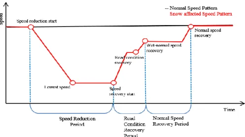
In Section 4.2.1, general descriptions of the speed variation process during snow events will be represented. Based on the results, three types of periods within the speed variations will be determined including: speed reduction period, road condition recovery period and normal speed recovery period. Through Sections 4.2.2 to 4.2.3, detailed analyses on the traffic flow patterns will be conducted for each distinctive period in the speed variations. In Section 4.2.5, the six phase change points will be determined in the traffic flow process during snow events.
4.2.1.Speed Variations Process during Snow Events
Based on the analysis of snow-affected traffic speed process, two types of patterns were identified with different conditions of traffic volumes in the sections. The typical pattern of snow-affected traffic flow variations during off-peak times is shown in Figure 9 and the case during peak times is shown in Figure 10.
In both cases, speed began to deviate from the dry-normal pattern after the snow event was initiated. Speed reached its minimum level as road conditions became worse. Speed increased as road conditions started to improve, due to the snow plowing operations executed within the given section. The durations and the patterns of the recovery were distinct in nature, depending on the methods of snow plowing operations and the variations in precipitation.
As shown in Figure 9, the bare lane-regain conditions allowed the speed to continue increasing up to the posted speed limit of the section as long as traffic was not congested.
After that point, speed remained at sustained levels for a while above the speed limit, but less than the dry-normal speed when wet conditions were obtained for the section. In turn, speed increased to dry normal levels when the road eventually became dry.
On the contrary, when traffic was congested during road recovery, speed began to decrease before reaching the posted speed limit because of traffic congestion, as shown in
Figure 10. This type of case imposes difficulties in estimating road surface conditions.
Figure 9: Phase Change Points in Traffic Flow Variations of 94 EB Snow Section during snow events on January 14, 2012 (Normal: black / Snow: red)
Figure 10: Phase Change Points in Traffic Flow Variations of 94 EB Snow Section during snow events on January 20, 2012
30 40 50 60 70 80 09: 30:00 09: 48:00 10: 06:00 10: 24:00 10: 42:00 11: 00:00 11: 18:00 11: 36:00 11: 54:00 12: 12:00 12: 30:00 12: 48:00 13: 06:00 13: 24:00 13: 42:00 14: 00:00 14: 18:00 14: 36:00 14: 54:00 15: 12:00 15: 30:00 15: 48:00 16: 06:00 16: 24:00 16: 42:00 17: 00:00 17: 18:00 17: 36:00 17: 54:00 18: 12:00 18: 30:00 18: 48:00 19: 06:00 19: 24:00 19: 42:00 20: 00:00 20: 18:00 20: 36:00 20: 54:00 21: 12:00 21: 30:00 21: 48:00 22: 06:00 22: 24:00 22: 42:00 Sectio n Sp ee d (m ph )
Average Normal Dry Snow Day (Jan. 14. 12)
15 25 35 45 55 65 75 85 05: 06:00 05: 24:00 05: 42:00 06: 00:00 06: 18:00 06: 36:00 06: 54:00 07: 12:00 07: 30:00 07: 48:00 08: 06:00 08: 24:00 08: 42:00 09: 00:00 09: 18:00 09: 36:00 09: 54:00 10: 12:00 10: 30:00 10: 48:00 11: 06:00 11: 24:00 11: 42:00 12: 00:00 12: 18:00 12: 36:00 12: 54:00 13: 12:00 13: 30:00 13: 48:00 14: 06:00 14: 24:00 14: 42:00 15: 00:00 15: 18:00 15: 36:00 15: 54:00 16: 12:00 16: 30:00 16: 48:00 17: 06:00 17: 24:00 17: 42:00 18: 00:00 18: 18:00 18: 36:00 Sectio n Sp ee d (m ph )
Average Normal Dry Snow Day (Jan. 20. 12) Snow Starting Time Snow Ending Time Snow Starting Time Snow Ending Time
For each case, the above patterns were represented in the schematic diagrams in Figure 11 and Figure 12 below. It should be noted that the road condition recovery process cannot only be identified in the speed variations when traffic is congested during road recovery. The traffic flow patterns during three types of periods will be discussed in greater detail in the following sections.
Figure 11: General Process of Snow-affected Speed Variations during Off-peak Time
4.2.2.Traffic Flow Process during the Speed Reduction Period
Within the stage of speed reduction, three types of patterns were identified depending on traffic volumes and precipitation intensity at the beginning of snow events. Each type of reduction pattern will be discussed in the sections to follow.
Type 1 Reduction Pattern: Both K and U decrease
Type 1 Reduction Pattern was characterized by the traffic flow behaviors that both speed and density decreased after the speed reduction starting point, as shown in Figure 13. This type was primarily observed in the case with diminishing traffic volumes during off-peak times. The patterns were observed regardless of the intensity of snow precipitation.
Figure 13: Type 1 Reduction Pattern: Speed decreases with decreasing density
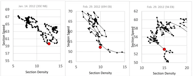
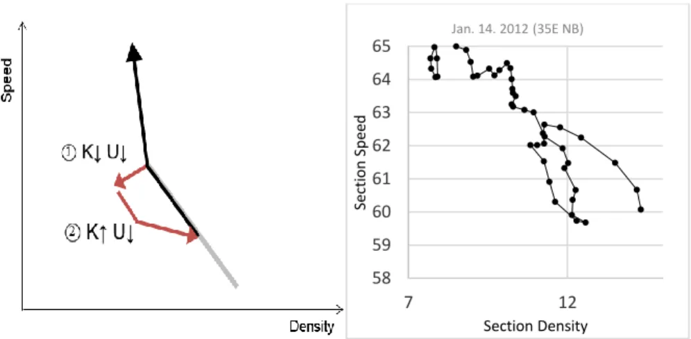
Type 2 Reduction Pattern: K increases and U decreases
The Type 2 Reduction Pattern was characterized by traffic flow behaviors that speed decreased with increasing density after the speed reduction starting point as shown
50 55 60 65 70 0 5 10 15 20 Se ct io n Spe ed Section Density Feb. 28. 2012 (35E SB) 50 55 60 65 70 75 80 0 5 10 15 20 Se ct io n Spe ed Section Density 2013.3.15, 694 EB 50 55 60 65 70 75 0 5 10 15 20 Se ct io n Spe ed Section Density 2013.3.15 @ 35E SB
in Figure 14. After the speed reduction starting point, it was observed that the density increased even at similar levels of traffic volume variations within the section. This was caused by the tendency of drivers to attempt to maintain an original level of flow rate. However, in most cases, a significant amount of speed reduction resulted in a decrease in flow rate even at increased density.
The Type 2 Pattern was predominantly observed during snow event cases with light precipitation, which explains the tendency of drivers under light snow precipitation to avoid hesitation in decreasing gap distance from the preceding vehicle in an attempt to maintain the original throughput in compensation of reduced speed due to snow.
Figure 14: Type 2 Reduction Pattern: Speed decreases with increasing density
Type 3 Reduction Pattern: K sustains while U increases
The Type 3 Reduction Pattern was characterized by traffic flow behaviors where speed decreased with sustaining density under conditions of heavy precipitation. This type
40 50 60 70 80 90 0 5 10 15 Se ct io n Spe ed Section Density 2013.2.3 @ 35E SB 40 50 60 70 80 90 0 5 10 15 Se ct io n Spe ed Section Density 2013.2.3 @ 694 EB 40 50 60 70 80 90 0 5 10 15 Se ct io n Spe ed Section De sity 2013.2.10 @ 694 EB
of pattern was predominantly captured during the high intensity of snow events, i.e., relatively lower average temperatures and a high level of accumulation of snow on the road.
Figure 15 shows the typical patterns of Type 3 Reduction Pattern. As shown in the figure, it was observed that after the speed reduction starting point, the density level sustained its value during speed reduction. This traffic flow pattern reflects the drivers’ behavior against the onset of significant snow events where drivers tend to maintain gap distance from the preceding vehicle while they decrease their speed because of snow. During intense weather conditions, drivers are prone to become cautious and hesitant, in order to maintain gap distance from the preceding vehicles, which resulted in the vertical decreasing speed reduction pattern in the SFD.
Figure 15: Type 3 Reduction Pattern: Speed decreases with sustaining density
Based on the analysis, three types of speed reduction patterns and the factors resulting from each type were identified, as shown below. In the schematic diagrams in Figure 16, if traffic volume was trivial, both speed and density decreased regardless of
40 45 50 55 60 65 70 75 0 5 10 15 20 25 Se ct io n Spe ed Section Density Nov. 19. 2011, 35E NB 40 45 50 55 60 65 70 75 0 5 10 15 20 25 30 Se ct io n Spe ed Section Density Nov. 19. 2011, 35E SB 60 62 64 66 68 70 72 74 0 5 10 15 20 25 Se ct io n Spe ed Station Density Jan. 14. 2012, 35E SB