Localization in Wireless Sensor
Networks (WSNs)
by
Hemat Kumar Maheshwari
Submitted in accordance with the requirements for the degree of Doctor of Philosophy
The University of Leeds
School of Electronic and Electrical Engineering
June, 2011
The candidate confirms that the work submitted is his own and that appropriate credit has been given where reference has been made to
the work of others.
The copy has been supplied on the understanding that it is copyright material and that no quotation from the thesis may be published
Like any research project, this work would not have been possible without the great support of my supervisor Dr. Andrew Kemp. I owe deepest gratitude to him for his contagious assistance and regular supervision meetings, which provided me the freedom to explore the new ideas. I would like to thank Prof. JMH Elmirghani and Dr. Ian Glover for their constructive feedback towards my research. I appreciate Colin Faulkner and Ivan Lawrow from NXP (Jennic) Ltd for their support during this research.
My four years at University of Leeds were simply remarkable and for that I would like to thank my WSN research group members. It was great to share my setbacks and successes with friends inside and outside the professional environment. I also extend my thanks to Mrs. A De Jong for her friendly assistance and making things simpler. Here, I would mention one person whose care and encouragement made my restless days and weekends simple and easy during the whole period of my research, my wife Raj Kumari. Thank you so much Raj, especially for your thoughtful attitude, delicious cooking, and wonderful company during all the trips and above all your trust and patience provided me a constant source of motivation.
Finally, I would especially like to thank my dearest grandparents, Dad and Mom for their endless support, blessings and teaching me values that are precious, irrespective of time and place. Special thanks and love to my brothers, sisters and in-laws for their encouragement and well wishes. They provide a constant source of motivation in my life.
&
lovely wife Raj Kumari.
The adoption of wireless sensor networks (WSNs) in numerous emerg-ing applications have prevailed us to realize that smart living is no
longer an imagination, it already exists. In emerging applications,
lo-calization is an essential function so that all the sensed information can be responded carefully. Among the range free and range aware localization, range aware localization has been the most promising for fine-grained accuracy. Range aware localization has two phases, rang-ing and localization. Location errors always exist no matter which ranging or localization technique is used. Therefore, there is a need to optimize range aware localization for better performance.
Firstly, this thesis investigates the performance of time-of-flight (ToF) and received signal strength (RSS) based ranging using IEEE 802.1.5.4 compliant WSNs nodes in outdoor and indoor for both line-of-sight (LOS) and non-line-of-sight (NLOS) paths. The fundamental Cram´e r-Rao lower bound (CRLB) on ToF and RSS ranging performance is compared with the performance limits of IEEE 802.1.5.4 compliant modules. The experimental results for both outdoor and indoor LOS path demonstrated that RSS is a good candidate for range estimation at ranges less than 7m. Further analysis over long range demonstrates that ToF is a good candidate for range estimation at greater than 7m. In addition to the ranging error, another well-known error mechanism is the poor geometric anchors placement, which can significantly de-grade localization performance. In the Global Positioning System (GPS) community, geometric dilution of precision (GDOP) is a well-known problem which illustrates the geometric configuration impact-ing localization accuracy. To analyse the impact of anchor placement
that lateration based approaches presents a trade-off for complex com-putation, thus energy consumption and accuracy. It provided the needed motivation to investigate and optimize the anchor placement for better localization accuracy. The impact of anchor placement for quality reliable localization has been limited to 3-4 anchors with re-spect to a single subject node for 2-D. Therefore, to model reality most clearly, it makes sense to step beyond the easy and secure reach of unrealistic and mostly researched 2-dimensional representations to the pragmatic world in 3-dimensional visualization. In addition, pre-vious work for optimal anchors placement has been limited to only additive noise. To the best of our knowledge, there is no study of optimization of anchor placement with respect to the multiplicative noise. Therefore, the optimal anchor placements are determined for both signal models based on minimum mean CRLB (m-CRLB). It is confirmed that optimal anchor placement for both signal models is different and have a serious impact on localization accuracy. The op-timal anchor placement is further verified by developing a new Range Aware Localization System (RALS) using IEEE 802.15.4 compliant devices.
In LOS, quality reliable localization performance can be achieved but as propagation criteria change from LOS to NLOS, localization per-formance also changes. In an indoor environment, localization perfor-mance degrades significantly due to multipath components. To over-come, a new 3-D scheme named Range Estimate Threshold (RET) is proposed which exploits field dimensions based on the signal model and optimal anchor placement to define a threshold. Based on the defined threshold, RET mitigates the poor range estimates from
Mea-sured Estimation(ME) for better localization accuracy. The
ramifica-tion of RET on ME is explored through additive, multiplicative and log-normal shadowing models. It is confirmed that localization based on RET compared to ME showed improved accuracy.
Acknowledgements i
Dedication ii
Abstract iii
List of Figures xi
List of Tables xxii
Abbreviations xxiii
Symbols xxvii
1 Introduction 1
1.1 Introduction . . . 1
1.2 Localization for Wireless Sensor Networks . . . 3
1.3 Scope and Motivations . . . 4
1.4 Contributions of the Dissertation . . . 9
1.5 Outline of the Dissertation . . . 10
1.6 Publications . . . 13
2 Background and Related Work 15 2.1 Introduction . . . 15
2.2 Localization in WSNs . . . 16
2.3 Classification of Localization . . . 17
2.3.1.1 Angle of Arrival (AoA) . . . 17
2.3.1.2 Complexity and Error Concerns using AoA . . . 18
2.3.1.3 Time Difference of Arrival (TDoA) . . . 18
2.3.1.4 Time of Flight (ToF) . . . 19
2.3.1.5 Received Signal Strength (RSS) . . . 19
2.3.2 Position Computation Phase . . . 21
2.3.3 Localization Algorithms . . . 21
2.4 Localization Techniques and Optimization . . . 26
2.4.1 Maximum Likelihood algorithm (ML) . . . 28
2.4.2 Approximate Maximum Likelihood algorithm (AML) . . . 29
2.5 Performance metric . . . 30 2.5.1 Accuracy . . . 30 2.5.2 Precision . . . 31 2.5.3 Complexity . . . 31 2.5.4 Robustness . . . 33 2.5.5 Scalability . . . 33 2.5.6 Cost . . . 33 2.6 Localization Systems . . . 33 2.6.1 Active Badge, 1992 . . . 33 2.6.2 Active Bat, 1999 . . . 34 2.6.3 Cricket, 2000 . . . 34 2.6.4 RADAR, 2000 . . . 35 2.6.5 Horus, 2005 . . . 35 2.6.6 SpotON, 2001 . . . 35 2.7 Applications . . . 35 2.7.1 Kid-Spotter . . . 36
2.7.2 Freight containers Positioning . . . 36
2.7.3 Asset Tracking and Management . . . 36
2.7.4 Aid to fire-fighters and police . . . 37
2.7.5 Detecting and Locating Radiation Levels . . . 37
2.7.6 Smart and Interactive Gaming . . . 37
2.7.7 Habitat Monitoring and Wildlife Tracking . . . 37
3 Performance Analysis of Ranging with IEEE 802.15.4 Compliant
WSN Devices 39
3.1 Overview . . . 39
3.2 Introduction . . . 40
3.3 Sources of Ranging Error . . . 42
3.3.1 Systematic Parameter . . . 42
3.3.2 Radio Propagation . . . 43
3.3.2.1 Large Scale Fading Models . . . 43
3.3.3 Small Scale Fading Models . . . 44
3.3.3.1 Effect of Frequency Channel on Multipath Perfor-mance . . . 45
3.3.4 Thermal Noise . . . 46
3.4 Experimental Infrastructure . . . 47
3.4.1 Antenna Models . . . 48
3.4.1.1 Integrated Folded Mono-pole Antenna . . . 49
3.4.2 Experimental Setup for Ranging . . . 49
3.4.2.1 Outdoor Experimental Setup . . . 50
3.4.2.2 Indoor Experimental Setup . . . 51
3.5 Round-Trip Time-of-Flight (RT-ToF) . . . 51
3.5.1 Principle of Operation . . . 54
3.5.2 RT-ToF Range Resolution . . . 55
3.5.3 Cram´er-Rao Lower Bound of ToF . . . 56
3.6 RSS: Principle of Operation . . . 59
3.6.1 Cram´er-Rao Lower Bound of RSS . . . 61
3.7 Site Survey and Analysis . . . 62
3.7.1 Successful ToF . . . 62
3.7.2 Remote Time Value Invalid . . . 63
3.7.3 Local Time Value Invalid . . . 63
3.7.4 No Acknowledgement . . . 63
3.7.5 No Data From Remote Node . . . 63
3.8 Experimental Results and Analysis . . . 66
3.8.1 Cross-over Range (CR) . . . 76
4 Localization using Optimal and Sub-Optimal Multi-lateration 79
4.1 Overview . . . 79
4.2 Introduction . . . 80
4.3 Signal Model . . . 81
4.4 Sub-Optimal Blind Trilateration (SBT) . . . 83
4.4.1 Least Squares Solution . . . 85
4.5 Geometric Dilution of Precision (GDOP) . . . 90
4.5.1 Simulation Results and Analysis . . . 99
4.6 Modified Sub-Optimal Blind Trilateration (MSBT) . . . 102
4.7 Optimal Multi-lateration (OML) . . . 106
4.8 Performance Analysis and Results . . . 111
4.8.1 Impact of Ranging Error . . . 113
4.8.2 Impact of Node Density . . . 116
4.8.3 Impact of Anchor Nodes on Localization Accuracy . . . 117
4.8.4 Analysis of Computational Complexity . . . 119
4.9 Discussion . . . 122
4.10 Summary . . . 122
5 The Optimization of Range Derived Localization in 2D and 3D WSNs 124 5.1 Overview . . . 124
5.2 Introduction . . . 125
5.3 Signal Models . . . 126
5.3.1 Multiplicative Noise Model . . . 128
5.4 Lower Bounds On Localization Error . . . 129
5.5 Optimal Anchor Placement for Minimum CRLB . . . 131
5.5.1 Two-Dimensional (2-D Case) . . . 131
5.5.2 Three-Dimensional (3-D Case) . . . 133
5.6 Optimal Anchor Placements . . . 136
5.6.1 Two-Dimensional (2-D) Case . . . 137
5.6.1.1 Optimal Anchor Placement for Additive Noise Model140 5.6.1.2 Optimal Anchor Placement for Multiplicative Noise Model . . . 146
5.6.1.3 CRLB Analysis of Anchor Node Constraints in 2-D152
5.6.2 Three-Dimensional (3-D) Case . . . 155
5.6.2.1 Optimal Anchor Placement for Additive Noise Model155 5.6.2.2 Optimal Anchor Placement for Multiplicative Noise Model . . . 159
5.6.2.3 CRLB Analysis of Anchor Node Constraints in 3D 162 5.7 Discussion . . . 163
5.8 Conclusion . . . 165
6 Localization Performance at Optimized Anchor Placement 166 6.1 Introduction . . . 166
6.2 2-D Case: Additive and Multiplicative Noise Model . . . 170
6.3 3-D Case: Additive and Multiplicative Noise Model . . . 175
6.4 Conclusion . . . 179
7 Experiencing RALS 181 7.1 Introduction . . . 181
7.2 Principle of Operation . . . 182
7.3 Experimental Infrastructure and Setup . . . 183
7.3.1 Indoor Setup . . . 184
7.4 Localization Performance Analysis . . . 186
7.4.1 Arbitrary Anchor Placement . . . 190
7.5 Summary . . . 191
8 Range Aware 3-D Localization in Indoor WSNs 192 8.1 Introduction . . . 192
8.2 Geometric Dilution of Precision Test for 3-D Setup . . . 195
8.3 Received Signal Strength . . . 199
8.4 Calibration of Path loss Exponent . . . 201
8.4.1 Training Phase . . . 202
8.4.1.1 Experimental Infrastructure and setup . . . 202
8.4.1.2 Formulation of Lookup Table . . . 206
8.4.2 Estimation Phase . . . 208
8.5.1 RET Algorithm Description . . . 212
8.6 Results and Analysis . . . 216
8.6.1 Simulation Case 1 : Lab-262b . . . 217
8.6.2 Simulation Case 2: Lab-160 . . . 226
8.7 Conclusion . . . 230
9 Conclusions and Future Research 232 9.1 Conclusions . . . 232
9.2 Future Research and Improvements . . . 236
9.2.1 Cooperative Localization (Extension to chapter 4) . . . 236
9.2.2 Additive/Multiplicative noise model . . . 237
9.2.3 Gaussianity assumption . . . 237
9.2.4 Path loss Exponent (η) . . . 238
9.2.5 Optimal anchor placement . . . 238
9.2.6 Experiencing RALS . . . 239
9.3 Sectorization Using Optimal Anchor Placement . . . 239
1.1 Fig. 1.1(a). Smart Sensor Architecture [1]. Fig. 1.1(b). JN5148 Micro-controller and sensor board [1]. . . 2
2.1 Location Stack [2] . . . 17
2.2 Fig. 2.2(a). Subject node with 3 in-range anchor nodes with actual ranging. Fig. 2.2(b). Subject node with 3 in-range anchor nodes with noise range. . . 27
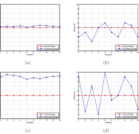
2.3 Precision and Accuracy analysis for randomly selected data: Fig.
2.3(a). High accuracy with high precision, Fig. 2.3(b). High ac-curacy with low precision, Fig. 2.3(c). Low accuracy with high precision, Fig. 2.3(d). High accuracy with low precision. . . 32
3.1 Integrated Folded Mono-pole antenna measurement planes [3]. Fig. (a). XY-Plane Fig. (b). XZ-Plane Fig. (c). YZ-Plane . . . 49
3.2 Measured antenna radiation pattern [3]. Fig. 3.2(a). XY-plane radiation pattern polar plot, Fig. 3.2(b). XZ-plane radiation pat-tern polar plot and Fig. 3.2(c). YZ-plane radiation pattern polar plot . . . 50
3.3 Outdoor experimental setup with two nodes, tripods and data log-ger laptop for range measurements. . . 51
3.4 Indoor experimental setup with two nodes, tripods and data logger laptop for range measurements. . . 52
3.5 Time-of-Flight (ToF) measurement. . . 53
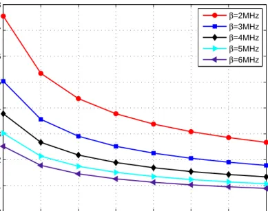
3.7 Impact of SNR and β on the fundamental CRLB for ToF ranging using IEEE 802.15.4 and UWB. . . 57
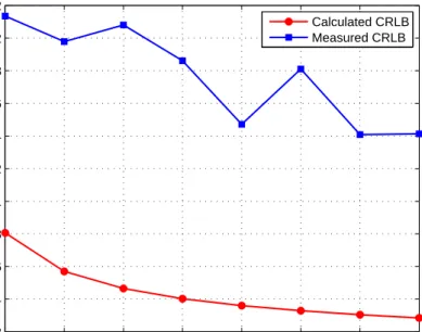
3.8 The Fundamental CRLB and measured performance limit of Jen-nic JN5148 series ranging module for ToF ranging . . . 58
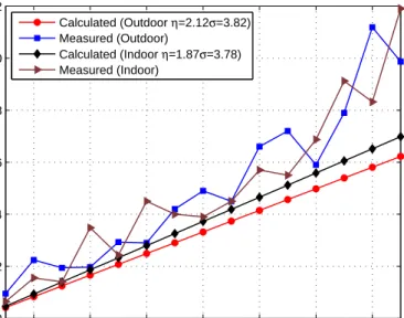
3.9 RSS versus range for measured data and path loss model. Fig.
3.9(a). Outdoor LOS at antenna height of 1.5m. Fig. 3.9(b). Indoor LOS at antenna height of 1.5m. . . 61
3.10 The fundamental CRLB limit and measured performance limit of Jennic JN5148 series ranging module for RSS. . . 62
3.11 Comparison of failed ToF polls taking quiet and busy channel in the account for indoor and outdoor LOS environment (height=1.5 m). (a, b). Quiet Channel in Outdoor and Indoor. respectively (c, d). Busy Channel in Outdoor and Indoor respectively. . . 65
3.12 Fig. (a). ToF estimated range in outdoor LOS path for different antenna heights. Fig. (b). ToF estimated range in indoor LOS path for different antenna heights. . . 67
3.13 Fig. (a). RSS estimated range in outdoor LOS path for different antenna heights. Fig. (b). RSS estimated range in indoor LOS path for different antenna heights. . . 68
3.14 ToF versus RSS estimated range in outdoor and indoor LOS path for antenna height of 1.5m . . . 68
3.15 ToF versus RSS estimated range in outdoor and indoor NLOS path for antenna height of 1.5m . . . 70
3.16 ToF estimated range in outdoor and indoor over long range for antenna height of 1.5m . . . 70
3.17 RSS estimated range in outdoor and indoor for antenna height of 1.5m . . . 71
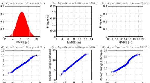
3.18 ToF and RSS: MMRE percentage in outdoor and indoor for LOS and NLOS paths over short range with antenna height of 1.5m. . 72
3.19 ToF and RSS: MMRE percentage in outdoor and indoor for LOS and NLOS paths over long range with antenna height of 1.5m. . . 73
3.20 PDF and Q-Q plot across ToF measurements over short range for outdoor LOS. . . 74
3.21 PDF and Q-Q plot across RSS measurements over short range for
outdoor LOS. . . 74
3.22 PDF and Q-Q plot across all of the ToF and RSS measurements over short range for outdoor NLOS. . . 75
3.23 Cross-over Range using experimental parameters. . . 77
4.1 Subject node with 3 in-range anchor nodes . . . 84
4.2 Subject node with 3 in-range anchor nodes . . . 85
4.3 Fig. 4.3(a). Subject node with 3 in-range collinear anchor nodes. Fig. 4.3(b). Subject node with 2 in-range anchor nodes, where 3 anchor nodes are co-incident. . . 89
4.4 Fig. 4.4(a). Anchor combinations, where A1, A2 are fixed anchors and anchor A3 is changed from A3 to A13. Fig. 4.4(b). ERMS as-sociated with the position estimate for different anchor geometries as shown in Fig. 4.4(a). Fig. 4.4(c) - Fig. 4.4(h). First 6 anchor combinations from Fig. 4.4(a), whereA1,A2 are fixed anchors and anchor A3 is changed from A3 to A8 respectively. . . 91
4.5 Simulation Flow chart for SBT . . . 92
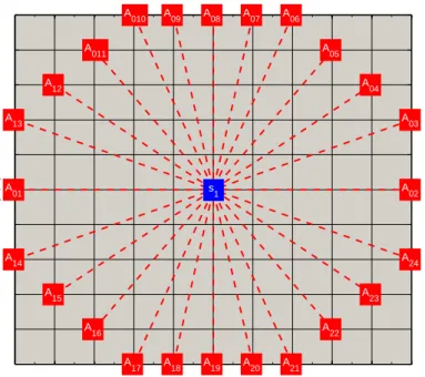
4.6 Subject node with 24 in-range anchors/pseudo-anchors, whereA1, A2 are fixed and A3 is changed from A3 to A24 . . . 100
4.7 Comparison of GDOP and ERMS for 24 in-range anchor nodes, whereA1,A2 are fixed andA3 is changed fromA3 toA24 as shown in Fig. 4.6. . . 100
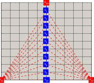
4.8 Subject node with 3 in-range anchors/pseudo-anchors, where A1, A2, A3 are fixed and sj is changed from s1 tos10. . . 101
4.9 Comparison of HDOP andERMSfor 3 in-range anchor nodes, where A1, A2, A3 are fixed and sj is changed froms1 tos10 as shown in Fig. 4.8. . . 102
4.10 Subject node with 3 in-range anchor nodes, where A1, A2, A3 are fixed and sj is changed from s1 to s21. . . 103
4.11 Comparison of GDOP andERMSfor 3 in-range anchor nodes, where A1, A2, A3 are fixed and sj is changed froms1 tos21 as shown in Fig. 4.10. . . 103
4.12 Subject node with 5 in-range anchor/pseudo-anchor nodes. . . 106
4.13 Possible anchor/pseudo-anchor node combinations. . . 107
4.14 Simulation Flow chart for MSBT. . . 108
4.15 Comparison of HDOP and ERMS for all anchor combinations as
shown in Fig. 4.13. . . 109
4.16 Optimal multi-lateration, where 8 anchor/pseudo-anchor nodes are in-range of a subject node. . . 109
4.17 HDOP and ERMS for OML, where 8 anchor/pseudo-anchor nodes
are in-range of a subject node as shown in Fig. 4.16. . . 111
4.18 Simulation Flow chart for OML. . . 112
4.19 Fig. 4.19(a). Example of simulation setup for 3 anchors (red squares), subject nodes (blue circles). Fig. 4.19(b). Example of simulation setup for 3 anchors (red squares), subject nodes (blue circles), and estimated subject nodes (yellow, pink, cyan and green squares) from each localization phase. . . 114
4.20 Impact of ranging error on average ERMS for 400 randomly
de-ployed nodes. . . 115
4.21 Impact of node density on averageERMS atσ2 = 0.5m. . . 116
4.22 Average number of Anchors/Pseudo-Anchors with respect to Node Density (σ2 = 0.5m). . . . 117
4.23 Impact of the number of Anchors/Pseudo-Anchors on averageERMS
(σ2 = 5m) in 200m by 200m network. . . . 118
4.24 Impact of the number of Anchors/Pseudo-Anchors on averageERMS
(σ2 = 10m) in 200m by 200m network. . . . 118
4.25 Impact of possible combinations of anchors/pseudo-anchors on av-erage RMS location error for 100 randomly deployed nodes (trans-mission range = 40m, σ2 = 0.5m) for MSBT. . . . 119
4.26 Average simulation time for single iteration of computation in 400m by 400m network with transmission range of 100m . . . 120
4.27 Impact of possible combinations of anchors/pseudo-anchors on av-erage computation time for 100 randomly deployed nodes (trans-mission range = 40m, σ2 = 0.5m) for MSBT. . . . 121
5.1 Fig. 5.1(a). Effects of additive noise model on the estimated range at noise variance of 2 and 4. Fig. 5.1(b). Effects of additive noise model on the estimated range at noise variance of 6 and 8. . . 127
5.2 Effects of Multiplicative noise model on the estimated range. Fig.
5.2(a). For κ=0.005, η=2 and 2.4. Fig. 5.2(b). For κ=0.005,
η=2.8 and 3.2. Fig. 5.2(c). For κ=0.5, η=2 and 2.4. Fig. 5.2(d). For κ=0.8,η=2.8 and 3.2. . . 130
5.3 Geometric relationship between two nodes in 2-D space. . . 131
5.4 Geometric relationship between two nodes in 3-D space. . . 133
5.5 Fig. 5.5(a) Relationship between possible combinations of anchor placements and 3×3 field dimensions. Fig. 5.5(b). Relationship between possible combinations of anchor placements and 4×4 field dimensions. . . 138
5.6 m-CRLB Flow Chart. . . 139
5.7 CRLB of all possible anchor combinations (placements) for a single subject location. . . 140
5.8 Optimal anchor placement for additive noise model in a 11×11 2-D plane for 3 to 8 anchors. . . 141
5.9 Optimal anchor placement and corresponding m-CRLB for addi-tive noise model using 3 to 8 anchor nodes as shown in Fig. 5.8(a)
- Fig. 5.8(f) for deployed subject nodes on a 11×11 2-D plane. Fig. 5.9(a). Impact of anchor nodes on m-CRLB. Fig. 5.9(b) -Fig. 5.9(g). contour plots for 3 to 8 anchors in 2-D for σ2 = 2. . . 142
5.10 Optimal anchor placement for 8 anchor nodes for three different scales. Fig. 5.10(a). For 21×21. Fig. 5.10(b). For 31×31. Fig.
5.10(c). For 41×41. . . 143
5.11 Worst anchor placement for additive noise model in a 11×11 2-D plane for 3 to 8 anchors. . . 144
5.12 Contour plot of worst anchor placement and corresponding m-CRLB for additive noise model for 3 to 8 anchor nodes. . . 145
5.13 Arbitrary anchor placement and corresponding minimum m-CRLB for multiplicative noise model using 3 - 8 Anchor nodes as shown in Fig. 5.8(a) - Fig. 5.8(f) (optimal for additive noise model) for deployed subject nodes on a 11×11 2-D space for η = 2 and κ = 0.001. . . 146
5.14 m-CRLB for multiplicative noise model as a function of the number of anchor nodes placed at the optimal positions for additive noise model. . . 147
5.15 Optimal anchor placement for multiplicative noise model in a 4×4 2-D plane for 3 to 8 anchors, where κ= 0.001 and η= 4. . . 148
5.16 Optimal anchor placement for multiplicative noise model in a 4×4 2-D plane for 3 to 8 anchors, where κ= 0.005 and η= 2. . . 150
5.17 Fig. 5.17(a)-Fig. 5.17(c). Optimal anchor placement for multi-plicative noise model in a 5×5 2-D plane for 3 to 6 anchors, where
κ = 0.001 and η = 4. Fig. 5.17(d)-Fig. 5.17(f). Optimal anchor placement for multiplicative noise model in a 6×6 2-D plane for 3 to 6 anchors, where κ= 0.001 and η = 2. . . 151
5.18 Optimal anchor placement and corresponding minimum m-CRLB at κ = 0.001 and η = 4 for multiplicative noise model using 3-5 anchor nodes for deployed subject nodes on 11×11 2-D plane. . . 151
5.19 Optimal anchor placement and corresponding minimum m-CRLB at κ = 0.001 and η = 4 for multiplicative noise model using 5 anchor nodes for deployed subject nodes on 21×21, 31×31 and 41×41 2-D space. . . 152
5.20 Worst anchor placement for multiplicative noise model in a 4×4 2-D plane for 3 to 8 anchors, where κ= 0.001 and η= 4. . . 153
5.21 Fig. 5.21(a). CRLB for 3 anchor nodes in 2-D, when anchor nodes are in a straight line (σ2 = 2 for all anchors). Fig. 5.21(b). CRLB
for 3 anchor nodes in 2-D, when two of the anchor nodes are co-incident (σ2 = 2 for all anchors). . . . 154
5.22 Optimal anchor placement for additive noise model in 3×3×3 3-D space for 4 to 6 anchors. . . 155
5.23 Optimal anchor placement for additive noise model in 11×11×11 3-D space for 4 to 8 anchors. . . 156
5.24 Optimal anchor placement and corresponding minimum m-CRLB for additive noise model for 4 to 8 Anchor nodes as shown in Fig.
5.23(a)- Fig. 5.23(e)for deployed subject nodes in 11×11×11 3-D space for σ2 = 2. . . . 157
5.25 Optimal anchor placement for 8 anchor nodes in 3-D for two dif-ferent scales. Fig. 5.25(a) for 5×5×5 scale. Fig. 5.25(b) for 12×12×12 scale. . . 158
5.26 Suboptimal anchor placement and corresponding minimum m-CRLB for multiplicative noise model using 4 - 8 Anchor nodes as shown in Fig. 5.23(a) - Fig. 5.23(e) for deployed subject nodes on a 11×11×11 3-D space for κ= 0.001 and η= 4. . . 160
5.27 Optimal anchor placement for multiplicative noise model in 3×3×3 3-D space for 4 to 6 anchors. Fig. 5.27(a) - Fig5.27(c). For κ = 0.005 andη = 2. Fig. 5.27(d)- Fig5.27(f). For κ= 0.001 and η= 4.161
5.28 CRLB for 4 anchor nodes in 3-D, where anchor nodes are placed on a single plane. . . 162
6.1 Fig. 6.1(a). Simulation setup in 2-D plane. Fig. 6.1(b). Simula-tion setup in 3-D space. . . 167
6.2 Arbitrary anchor placement 1 in 10×10 2-D space for 3 to 8 anchors.168
6.3 Arbitrary anchor placement 2 in 10×10 2-D space for 3 to 8 anchors.168
6.4 Arbitrary anchor placement 3 in 10×10 2-D space for 3 to 8 anchors.169
6.5 Performance of the LS method for additive noise model at optimal and arbitrary anchor placement and comparison with m-CRLB. . 171
6.6 Performance of the AML method for additive noise model at opti-mal and arbitrary anchor placement and comparison with m-CRLB.171
6.7 Performance comparison of LS and AML method for additive noise model at optimal and arbitrary anchor placement. . . 172
6.8 Performance comparison of LS and AML method for multiplicative noise model at additive’s optimal placement with arbitrary anchor placement. . . 173
6.9 Performance of the LS and AML method for multiplicative noise model for κ = 0.001 and η = 4 at optimal and arbitrary anchor placement and comparison with m-CRLB. Fig. 6.9(b). For 5×5, where optimal placement for multiplicative noise model is as shown in Fig. 5.17(a) - Fig. 5.17(c). Fig. 6.9(a). For 11×11, where
optimal placement for multiplicative is as shown in Fig. 5.18. . . . 174
6.10 Arbitrary anchor placement 1 in 10×10×10 3-D space for 4 to 8 anchors. . . 175
6.11 Arbitrary anchor placement 2 in 10×10×10 3-D space for 4 to 8 anchors. . . 176
6.12 Arbitrary anchor placement 3 in 10×10×10 3-D space for 4 to 8 anchors. . . 176
6.13 Performance of the LS method for additive noise model at optimal and arbitrary anchor placement and comparison with m-CRLB. . 177
6.14 Performance of the AML method for additive noise model at opti-mal and arbitrary anchor placement and comparison with m-CRLB.178 6.15 Performance comparison of LS and AML method for additive noise model at optimal and arbitrary anchor placement. . . 178
7.1 Flow Chart for PAN Coordinator node. . . 183
7.2 Flow Chart for Anchor nodes. . . 184
7.3 Flow Chart for Subject nodes. . . 185
7.4 Fig. 7.4(a). Localization testbed in a Lecture Theatre, where three anchors are optimally placed, whereas subject node is placed in the centre. Fig. 7.4(b). Jennic JN5148 controller board and LCD splash screen on the subject node. . . 186
7.5 Estimated subject coordinates and ERMS in cm, when anchors are optimally placed and subject node is placed at [3m,3m] as shown in Fig. 7.4(a). . . 187
7.6 Fig. 7.6(a). Estimated subject coordinates andERMS in cm, when
anchors are optimally placed and subject node is placed at [3m,0m]. Fig. 7.6(b). Estimated subject coordinates and ERMS in cm, when
7.7 Fig. 7.7(a). Three anchors are optimally placed, whereas subject node is placed at [3m,9m] outside of the triangle. Fig. 7.7(b). Corresponding ERMS(cm). . . 189
7.8 Fig. 7.8(a). Subject node estimated coordinates and ERMS when
three anchors are placed at arbitrary placement, whereas subject node is placed in the centre of the field ([3m,3m]). . . 190
8.1 7 different 3-D anchor placements according to the dimensions of Wireless Sensor Networks Research Group lab (262b) at University of Leeds. . . 197
8.2 Simulation setup for anchor placement 1 as shown in Fig. 8.1. . . 197
8.3 Impact of noise variance and anchor node placements on PDOP in 3-D context. . . 198
8.4 Impact of noise variance and anchor node arrangements on ERMS
in 3-D context (based on 3-D trilateration using LS method for 7 different anchor combinations and 50 randomly deployed subject nodes.) . . . 198
8.5 Profiling an area of interest by exploiting the link information (face diagonal) between pair of anchors in 3-D, where 4 anchors are optimally placed. . . 201
8.6 Fig. 8.6(a). Wireless Sensor Networks Research Group Lab (Lab-262b) in the School of Electronic and Electrical Engineering at the University of Leeds. Fig. 8.6(b). Computer Cluster Lab (Lab-160 in the School of Electronic and Electrical Engineering at the University of Leeds. Fig. 8.6(c). Node mounted on a tripod and connected to laptop via UART. Fig. 8.6(d). Node mounted with multi-purpose tac around the corner of the wall. Fig. 8.6(e). Ex-perimental setup along with anchor nodes arrangement 1. . . 203
8.7 Node placement for calibration of path loss exponent in Lab-262b. 204
8.8 Node placement for calibration of path loss exponent in Lab-160. . 205
8.9 Path loss exponent calibration process forAi wherei= 1, . . . , N. 205
8.10 RSSI ranging samples between each anchor and subject node 1 as shown in Fig. 8.7 (lab-262b). . . 207
8.11 Fig. 8.11(a). Lab-262b lookup table mapping using ηAi and ηµ as
shown in table 8.1 for each anchor node. Fig. 8.11(a). Lab-160 lookup table mapping using ηAi and ηµ as shown in table 8.1 for
each anchor node. . . 208
8.12 Subject node estimation using calibrated path loss exponent with respect to each anchor node Ai for i= 1, . . . , N. . . 209
8.13 Space and face diagonal between anchor Ai and subject sj nodes
in 3-D for RET. . . 210
8.14 Fig. 8.14(a). RET for additive noise model where σ2 = 1, 3, 5, 7,
and 9. Fig. 8.14(b). RET for multiplicative noise model where
κ= 0.001, 0.003, 0.005, 0.007, and 0.009. . . 212
8.15 Fig. 8.15(a). Space and face diagonals between anchors and sub-ject nodes in 3-D for RET of Lab-160. Fig. 8.15(b). RET for ad-ditive noise model whereσ2 = 1,3,5,7,and 9. Fig. 8.15(c). RET
for multiplicative noise model whereκ= 0.001,0.003,0.005,0.007,
and 0.009. . . 213
8.16 Extraction of poor range estimates ( ˆdpij) based on RET defined by using lab262b field dimensions and signal models. Fig. 8.16(a). Additive noise model. Fig. 8.16(b). Multiplicative noise model using ηµ. Fig. 8.16(c). Multiplicative noise model using ηAi. Fig.
8.16(d). RSS path loss model. . . 218
8.17 CDF comparison of ME and RET for additive and multiplicative noise models. . . 220
8.18 Comparison of ME and RET for additive and multiplicative noise models. Fig. 8.18(a). Additive noise model. Fig. 8.18(b). Multi-plicative noise model. Fig. 8.18(c). CDF comparison of ME and RET based on all samples at σ2 = 1,3, 5, 7, and 9 for additive
and κ = 0.001, 0.003, 0.005, 0.007, and 0.009 for multiplicative noise model from Fig. 8.17(a)- Fig. 8.17(e) for both additive and multiplicative noise models. . . 221
8.19 ERMS comparison for each node index for additive noise model.
8.20 ERMScomparison for each node index for multiplicative noise model.
Fig. 8.20(a) and Fig. 8.20(b). Using ηµ at κ = 0.001 and 0.007
respectively. Fig. 8.20(c)and Fig. 8.20(d). UsingηAi atκ= 0.001
and 0.007 respectively. . . 223
8.21 CDF comparison of ME and RET for CE based RSS localization using ηAi and ηµ in lab-262-b. . . 224
8.22 ERMS comparison for each node index for RSS path loss model
based on CE. Fig. 8.22(a) and Fig. 8.22(b). Using ηµ and ηAi
respectively. . . 225
8.23 Extraction of poor range estimates ( ˆdpij) based on RET defined by using lab169 field dimensions and signal models. Fig. 8.16(a). Additive noise model. Fig. 8.16(b). Multiplicative noise model using ηµ. Fig. 8.16(c). Multiplicative noise model using ηAi. Fig.
8.16(d). RSS path loss model. . . 226
8.24 Comparison of ME and RET using additive and multiplicative noise models for lab-160 dimensions. Fig. 8.24(a). Additive noise model. Fig. 8.24(b). Multiplicative noise model. Fig.
8.24(c). CDF comparison of ME and RET based on all samples at
σ2 = 1,3,5,7,and 9 for additive andκ= 0.001,0.003,0.005,0.007,
and 0.009 for multiplicative noise model. . . 227
8.25 CDF comparison of ME and RET for CE based RSS localization using ηAi and ηµ in lab-160. . . 229
8.26 ERMS comparison for each node index for RSS path loss model
based on CE. Fig. 8.26(a) and Fig. 8.26(b). Using ηµ and ηAi
respectively. . . 229
9.1 Fig. 9.1(a) - Fig. 9.1(c). Sectorization of localization field with respect to 3, 4 and 5 optimally placed anchor nodes for multiplica-tive noise model. Fig. 9.1(d). Simulation setup for sectorization with respect to 4 optimal placed anchors for multiplicative noise model. . . 241
3.1 Specification of IEEE 802.15.4 Compliant Devices . . . 48
3.2 Approximated Propagation Parameters . . . 60
3.3 Site Survey Results . . . 64
3.4 Site Survey Results . . . 66
3.5 Experimental Results: ToF Vs RSS . . . 69
4.1 Geometric Dilution of Precision Quality Rank . . . 93
4.2 Network Simulation Parameters for SBT, MSBT and OML . . . . 113
6.1 Network Simulation Parameters to analyse the anchor placement. 167
8.1 Calibrated Propagation Parameters . . . 206
List of Abbreviations
ACK AcknowledgementAML ApproximateMaximum Likelihood API Application Programming Interface APIT ApproximatePoint In Triangulation AWGN AdditiveWhite Gaussian Noise CCA Clear ChannelAssessment
CDF Cumulative Distribution Funciton CE Callibrated Estimation
CRLB Cram´er-Rao Lower Bound
CSMA-CA Carrier Sense Multiple Access with Collision Avoidance DoD Departmetn of Defence
DOP Dilution of Precision
DSSS Direct Sequence Spread Spectrum ED Energy Detection
FCC Federal Communications Commission FIM Fisher Information Matrix
GDOP Geometric Dilution of Precision GLONASS GLObal Navigation Satellite System GPS Global Positioning System
GPRS General Packet Radio Service HDOP Horizontal Dilution of Precision HSPA High SpeedPacket Access ID Distinctive Identification
IEEE Institute of Electrical andElectronics Engineers IETF Internet Engineering Task Force
ISM Industrial, Scientific and Medical LBS Location Based Service
LCD LiquidCrystal Display LoP Line of Position
LOS Line-of-Sight LS Least Squares
LTE Long-Term-Evolution
m-CRLB Mean Cram´er-RaoLower Bound MAC MediumAccess Layer
MATLAB MatrixLaboratory ME MeasuredEstimation
MEMS Micro-Electro-Mechanical System ML Maximum Likelihood
MLME Media Access Control (MAC) Sublayer Management Entity MMRE Magnitude of Mean Range Error
MP Multipath Propagation
MSBT Modified Sub-Optimal Blind Trilateration MSE Mean Square Error
NLOS Non-Line-of-Sight
O-QPSK OffsetQuadrature Phase ShiftKeying OML OptimalMulti-lateration
PCB Printed Circuit Board
PDF Probability Density Function PDOP Position Dilution of Precision
PN Pseudo-noise
PSD Power Spectral Density QoS Qualityof Service Q-Q Quantile-Quantile
RALS Range AwareLocalization Sytstem RBW Resolution BandWidth
RET Range EstimateThreshold RF Radio Frequency
RISC ReducedInstruction SetComputing RSS ReceivedSignal Strength
RSR RootSelection Routine RT-ToF Round-Trip - Time of Flight RTLS Real Time Location System SBT Sub-OptimalBlind Trilateration
SeRLoc Secure Range-Independent Localization SNR Signal-to-Noise Ratio
TDOA Time Difference of Arrival TEU Twenty-footEquivalentUnit
TLS TaylorSeries Expansion ToF Time of Flight
TRET Tamper Resistant Embedded Controller UART Universal AsynchronousReceiverTransmitter USB Universal Serial Bus
UWB Ultra-Wide-Band
VDOP VerticalDilutionof Precision VHF Very High Frequency
WiMAX Worldwide Iinteroperability for Microwave Access WLAN Wireless Local Area Network
WPAN Wireless Personal Area Network WSN Wireless Sensor Network
List of Symbols
Symbol Definition
α Orientation (Angle)
β Bandwidth
δ Dirac Delta Function
η Path Loss Exponent
ηAi Path Loss Exponent for Anchor i
ηµ Averaged Path Loss Exponent
ǫo Standard Normal Random Variable
σ2 Noise Variance 2-D 2 Dimensions 3-D 3 Dimensions At Path Amplitudes Ai ith Anchor Node AN Number of Anchor/Pseudo-Anchor Ac Anchor Combinations ˆ
Ac Selected Anchor Combination
Air Number of in-range Anchor/Pseudo-anchor Nodes
Symbol Definition
CAP Collinear Anchor Placement
cm Centimetre
CR Cross-over range
dBm Decibels related to 1 milliwatt
dij Distance between ith anchor and
jth subject node
ˆ
dij Estimated Distance ith anchor and
jth subject node
dxi Direction Cosines
dyi Direction Cosines
ERMS Root-Mean-Square-Error
ELoc
RMS Root-Mean-Square-Error for Localization
Er
RMS Root-Mean-Square-Error for Ranging
fs Clock Rate
Gr Receiver antenna gain
Gt Transmit antenna gain
GM Geometry Matrix
h Height
hr Receiver antenna height
ht Transmit antenna height
Hz Hertz
Symbol Definition
ℓi NLOS bias
l Length
J Objective function (AML)
k Number of iterations
kB Boltzmann’s constant
Kp Multiple paths
L System loss factor
M Number of subject nodes
m Metre
MSs Mobile Stations
MPL Maximum Possible Locations
N Number of anchor nodes
No Noise power spectral density
Np Noise power
n Error Function of Ranging System
Pr Receive power
Pt Transmit power
Rc Chip Rate
s Second
ˆ
s Estimated subject node
sj Subject node
Symbol Definition
SNRm Measured Signal-to-Noise-Ratio
Sr Symbol rate
τ Propagation Delay T Matrix transpose
T System temperature (Kelvin)
Tc Chip period
Tcor Correlation time estimate
Ttof Total Time-of-Flight
Ttot Total measure time
Ttat Total turn-around time
Trx Receive delay
Ts Symbol duration Time
Ttx Transmit delay
w Width
x x coordinated
y y coordinated
Introduction
1.1
Introduction
The last couple of decades have seen a tremendous development in micro-electro-mechanical-systems (MEMS), data communication and electronics. In 2002, it allowed researchers from Intel and UC Berkeley as a part of famous Great Duck Island project to monitor dozens of petrel’s nesting burrows with small devices calledmotes[4]. Each mote is about the size of its power source-a pair AA batter-ies (energy source), capable of performing some processing (equipped with pro-cessor), gathering sensory information (small memory), sensing and monitoring environment (light, humidity, pressure, and heat sensors). Above all, there was also a radio transceiver just powerful enough to cooperatively communicate with other connected neighbour motes in the network and to transmit monitored data. The motes, equipped with five main components as shown in figure1.1(a), reflect a future composed by networks of battery powered wireless sensors that monitor our environment, our machines and even us [4]. Fig. 1.1(b)shows 2.4GHz IEEE 802.15.4 and ZigBee PRO compliant JN5148 micro-controller and sensor board. It integrates an extremely powerful 32-bit RISC CPU with cumulative memory inside amounts to 256 kbyte, and, combined with efficient code utilization. This is enough for a full ZigBee PRO stack and to provide space for applications [1].
WSNs are very application specific networks and composed of a large num-ber of tiny sensors, which can be deployed over a vicinity of interest. Based on the type and purpose like continuous sensing and control, event detection and
(a) (b)
Figure 1.1: Fig. 1.1(a). Smart Sensor Architecture [1]. Fig. 1.1(b). JN5148 Micro-controller and sensor board [1].
identification, monitoring and surveillance they can be deployed in small scale or large scale networks. The deployment can be with the static constraint of nodes or considering the mobility based indoor or outdoor with unpredictable environmental factors. These sensor devices exhibit several limitations in terms of energy consumption, restricted computation capability, storage capability, sig-nal processing and short range radio communication [5]. Furthermore, WSNs differ from traditional wired and wireless networks in terms of the node density (i.e. large number of sensor nodes in a vicinity), sensor nodes deployment (i.e. unattainable or remote vicinities), dynamic and unpredictable node mobility (i.e. may leave or join the network) and node failure (i.e. due to lack of battery power). Therefore, to address these limitations, there is a need of efficient and optimized processing, which can reduce the communication cost.
Based on different characteristics as discussed above and application specific nature of WSNs, the field of WSNs exhibits many challenges. A detailed survey of different challenges is discussed in [5]. These challenges include, optimization of localization, energy efficient geographic routing, location aware security, data storage, location aware inter-node cooperation, data-dissemination incorporating localization, fault detection and tolerance and others. However, localization of nodes in such networks exhibit new challenges due to its integration with many emerging applications and system functionalities.
1.2
Localization for Wireless Sensor Networks
According to Technology Review magazine published by Massachusetts Institute of Technology (MIT), WSNs are one of the top ten technologies, which will change the world and the way we live our lives [4]. A wide variety of emerging applications are considered under the umbrella of WSNs such as, intelligent transport, biodi-versity mapping, robotic land-mine detection, battlefield surveillance, precision farming, disaster recovery operations, intelligent buildings, monitoring the flow of glaciers, critical coastal ecosystems, detect alpha, beta and gamma radiation and others. In many of these applications, determining the position of sensors is one of the top priorities. Since, WSNs are application oriented networks, the ultimate aim of location aware WSNs is to optimize the reliably and precision of location information for location based services (LBS). It is because that without the knowledge of geographic information, data passed by sensors is meaningless or without having the knowledge of location of an event it will be quite useless for LBS to reply in response to data received from the sensors. In addition, energy efficient geographic routing has shown great interest, where accurate and reliable localization is the first basic requirement [6]. Furthermore, system functionalities like network coverage checking and location-based information querying are de-pendent on the reliable localization [7]. It previews that; optimized localization can be further incorporated to optimize the communication mechanism in WSNs. Localization is used to solve the problem of determining the positions of nodes or objects. Localization in fact can be used to represents the relationship between different objects based on the coordination system. Due to the application specific nature and its integration with many systems functionalities, the localization ap-proaches in WSNs are classified as range-free [8–10] and range-based approaches [11–13]. The former is based on the topological relationship and does not utilize range estimation for localization. One of the main problems with range-free lo-calization is that this type of lolo-calization is suitable for relative location instead of fixed location as they use proximity information to estimate the location of the nodes in a WSN, and thus have limited precision. The latter approach (geomet-rical) is based on using angle estimates [14,15], or accurate range measurements, which can be derived from measuring point-to-point propagation time [16,17] orusing received signal strength [14]. This thesis addresses the challenge of range aware localization in WSNs.
1.3
Scope and Motivations
This section states the scope and impetus behind this research in WSNs with respect to each chapter.
• Motivation 1 - [Chapter 3]: The swift growth of wireless networking
in our daily life has forced the division of wireless applications into differ-ent standardization directions. One direction getting a lot of attdiffer-ention is the IEEE 802.15.4/Zigbee [18] global standard for short range, low-data-rate, low-power, and low-cost applications, which is intended to serve and be adopted by industrial, scientific and medical (ISM) applications. These features, differentiate IEEE 802.15.4/Zigbee standard with other standards such as Wireless Local Area Networks (WLAN), the ubiquitous Bluetooth devices, different versions of Worldwide Interoperability for Microwave Ac-cess (WiMAX) such as, fixed WiMAX (802.16d) for faster Wi-Fi style ISP networks, mobile WiMAX (802.16e) for use as a 3G/HSPA replacement by mobile phone operators and recently approved WiMAX2/WirelessMAN-Advanced (802.16m) standard for high-speed wide area wireless networking and Long Term Evolution (LTE) technology, which are expected to become the next major global wireless technology. However, all of these networks focused to achieve high data throughput and high quality of services (QoS) and it makes IEEE 802.15.4/Zigbee standard an ideal choice for WSNs re-search community for a wide range of applications as discussed above. In many of these applications, determining the position of sensors is one of the top priorities. An alternate to IEEE 802.15.4/Zigbee standard for lo-cation aware applilo-cation is Ultra-Wide-Band (UWB), which is developed by IEEE 802.15.4a Task Group [19] to meet sub-metre accuracy. How-ever, UWB is limited in operational range (< 100m) because of the Fed-eral Communications Commission (FCC) regulation on transmission power [20]. The UWB air interface, which is between 3.1GHz and 10.6GHz, has
attracted many wireless communication areas, including WSNs due to its lower power consumption, an increased data rate over comparatively short range, large bandwidth (minimum of 500MHz), superior performance in multipath environments, and realization of an ultra-low power with sim-ple and easy to design transmitters [21]. The poor ranging performance of non-coherent UWB receivers [22] (i.e. lack of synchronization, channel estimation and pulse shape estimation, energy detection, and interference) diverted research towards the fully coherent reception of UWB signals [23]. The performance of these coherent receivers is the result of relatively high computation and processing requirements, and hardware complexity [21]. The most common technique in locating a wireless device is the so called trilateration method. In the first phase of this technique, anchor nodes per-form ranging individually with the subject node and based on this range information, the second phase (localization phase) estimates the subject nodes coordinates. It suggests that ranging accuracy is an important as-pect to consider because a localization system obtains position estimates using range estimates. Inaccurate range estimation may lead to unaccept-able localization errors. Hence, for efficient localization, it is imperative to understand the performance limits of ranging in realistic environments. Two widely used methods for range estimation are the time-of-flight (ToF) and the received signal strength (RSS). Recently, commercial products have been released by several vendors such as Jennic [24], Dust Networks (win-ner of the best technical development of a WSN/RTLS device, May 2011, by DTechEx Energy Harvesting and WSN Awards) [25], Texas Instruments [26], Freescale semiconductor [27], and Atmel [28]. In late 2009, Jennic introduced IEEE 802.15.4 compliant devices with built-in ToF engine and RSS capability to revolutionize LBSs. It encouraged us to address the per-formance limits of ToF and RSS based ranging for IEEE 802.15.4 compliant devices in realistic environments. The indoor and outdoor experimental re-sults provided a platform to understand and demonstrate the performance behaviour of IEEE 802.15.4 ToF based ranging.
• Motivation 2 - [Chapter 4, 5 and 6]: The last couple of decades have
seen tremendous interest in research towards subject localization, where the subject position is to be determined from a set of noisy measurements. This work is mainly focused on range aware localization, where a set of measurement used to locate the subject node are range estimates between the subject and a set of fixed nodes (aka anchors). The range estimates can be obtained via time-of-flight (ToF) or received signal strength (RSS). Location errors always exist no matter which ranging technique is used. In addition to the ranging error (as discussed above), another well-known error source is the geometric placement of anchor nodes, which can significantly degrade the quality of position estimate based any localization technique. In NAVSTAR/Global Positioning System (GPS), and Global Navigation Satellite System (GLONASS) community, geometric dilution of precision (GDOP) is a well-known problem [29–36] which illustrates the geometric configuration impacting location estimation accuracy of a localization sys-tem. Previous work has shown that poor anchor placement can lead to a substantial degradation in the performance of any range aware localization technique in terms of accuracy. Although, several schemes and fixes have been proposed to mitigate the impact of anchor placement on range derived localization. However, there is little or limited work on the optimization of anchor nodes placement. The impact of anchor placement for precise and accurate localization have been limited to 3-4 anchor nodes with respect to a single subject node for 2-dimensions, hence no optimization of optimal sensor placement. Moreover, there is a comparatively little extension avail-able for optimal anchor placement in 3-dimensions. In addition to that, in terms of the signal model, previous work for geometric placement of anchors has been limited to only additive noise model. To the best of our knowl-edge, there is no study of geometric placement of anchor nodes with respect to the multiplicative noise model. The observation above encouraged us to investigate the optimization of optimal anchor placement for both additive and multiplicative noise models, moreover for both 2-D and 3-D scenarios. In addition, the above observation also motivates to obtain the
understand-ing of the impact of location error due to the geographic anchor placement for range derived localization in WSNs.
To understand the impact of geometric placement of anchor nodes, chapter
4presents the performance analysis of three localization methods. Different geometric anchor placements have shown the different impact on localiza-tion accuracy. Particularly, extensive simulalocaliza-tions try to discover the im-pact of anchors/pseudo-anchors geometry by varying the number of anchor nodes, node density and communication range. The study is expected to extend the finding of other studies, and also give new insight into optimal anchor placement. This comparative performance analysis of localization using optimal and sub-optimal lateration provided the needed motivation to optimize the anchor placement in order to enhance the performance of range aware localization.
Various techniques have been developed to solve the trilateration distance equations. These include the LS methods [37], the weighted LS method [38] and the maximum likelihood (ML) approach [39]. The performance of these algorithms is bounded by the Cram´er-Rao lower bound (CRLB) which is dependent on the geometry of the anchors and the target node. The limit on performance calculated in [40] is based on the additive noise model while a modified CRLB based on the multiplicative noise model is proposed in [41]. Noticeably, work in this area [42,43] has not considered the minimum mean CRLB (m-CRLB) to optimize the anchor placement. So it is believed that, it is the first study which takes minimum m-CRLB into consideration for both additive and multiplicative noise models for optimization of anchor placement in 2-D as well as in 3-D. It exposes new findings and problems, which have not been previously discovered or have been miss understood before due to the widely studied and focused additive signal model.
• Motivation 3 - [Chapter 7]:
The last couple of decades have seen tremendous interest in the implemen-tation of real time localization system (RTLS) using wireless sensor nodes, due to the fact that GPS cannot be connected with every single piece of
sensor node. An added challenge is the fact that in practice the real world is 3-D, which adds more complexity but on the same time demands for high accuracy. The localization systems that are implemented using wireless sen-sor networks (WSNs) are beacon-based localization [8], RSSI based SpotON [44], and RF and acoustic signal based Calamari [45]. However, these im-plemented wireless sensor networks are limited to 2-D. These systems are further discussed in chapter 2. The real sign of motivation here is to un-derstand the practical issues while deploying a real time location system, differentiation between the practical deployment and simulation world and moreover, to verify the impact of optimal anchor placement on a real time location system, which are derived in chapter 5. The range aware local-ization system (RALS) uses Jennic’s JN148 compliant devices with built-in RT-ToF ranging to locate a subject node in 3-D as well as in 2-D.
• Motivation 4 - [Chapter 8]: In recent years, there has been a great
in-terest in research towards positioning of wireless devices in confined areas. The Global Positioning System (GPS) [29] provides an excellent worldwide lateration framework for determining geographic position. GPS solution is famous for outdoor applications. However, this solution has several limi-tations, the major is of course the dependency on LOS reception, together with the high power requirement and hardware complexity from satellites. With such limitations GPS typically fails in harsh environments (i.e. inside homes, offices, shopping malls, underground and between heavy vegeta-tive cover) and exhibits suboptimal performance for WSNs. To overcome these limitations and to enhance localization accuracy, indoor positioning systems, based on the use of Global Navigation Satellite System (GNSS) repeaters [46], CarpetLAN [47] which is an indoor broadband-positioning system, infrared based active-badge system [48], or ultrasounds [49], have been developed. An overview on indoor application can be found in [50], which conclude that there is no optimal solution for positioning yet. While GNSS have become the dominating system for open-sky, several sys-tems share the indoor market; each having its own drawbacks, such as low accuracy, sophisticated infrastructures, limited coverage area or inadequate
acquisition costs [50]. However, their complexity, their power consumption, and their deployment costs are enduring problems [51]. To overcome, WSNs have found their way into a wide range of location based services (LBS) in-cluding indoor localization. Indoor localization has been a great interest in research because a reliable and accurate localization in harsh environ-ments is an integral part of many emerging applications including logistics, medical services (i.e. neonatal monitoring, patient tracking), enclosed in-door rescue operations (i.e. tunnels, caves, buildings), home automation, and others. In addition, efficient localization in confined areas helps to en-hance geographic routing and data dissemination for rescue operations. In ideal conditions (i.e. LOS case), quality reliable localization performance can be achieved but as propagation criteria change from ideal LOS to non-line-of-sight (NLOS), localization performance also changes. The localiza-tion performance degrades significantly in indoor environment, where range measurements include NLOS errors due to the excess path length caused by multipath propagation [52]. The estimated error in such harsh environ-ments is assumed to have a large positive bias that causes range estimates to be greater than the actual range. Such indoor environments fail a local-ization system to mark the required accuracy and therefore, highlight the indoor localization as a challenging problem. The observation above en-couraged us to present an attempt along this direction by proposing a new 3-D scheme namedRange Estimate Threshold(RET). The proposed scheme defines a RET based on the 3-D field dimensions and the signal noise model to mitigate the poor range estimates ( ˆdpij) fromMeasured Estimation(ME) to optimize range estimates.
1.4
Contributions of the Dissertation
The thesis focuses on the optimization of range aware localization in WSNs. The main novel contributions of this thesis are listed below and further explained in section 1.5:
• Performance analysis of round-trip time-of-flight (RT-ToF) and received
signal strength (RSS) for point to point range estimation using 2.4GHz IEEE 802.15.4 compliant transceivers (Chapter 3)
• Performance analysis of localization using sub-optimal blind lateration (SBT),
optimal multi-lateration (OML), and modified sub-optimal blind trilatera-tion (MSBT) based on knowledge of geometric dilutrilatera-tion of precision (GDOP) in cooperative fashion (Chapter 4)
• Optimal and worst anchor placements for additive and multiplicative noise
model in 2-D based on minimum mean Cram´er-Rao Lower Bound (m-CRLB) (Chapter 5)
• Optimal and worst anchor placements for additive and multiplicative noise
model in 3-D based on minimum mean Cram´er-Rao Lower Bound (m-CRLB) (Chapter 5)
• Localization performance for additive and multiplicative noise model at
different scales in 2-D and 3-D and their comparison with the lower bound for optimal, worst and arbitrary anchor placements (Chapter 6)
• Implementation of real time localization system 2.4GHz on Jennic’s JN5147
IEEE 802.15.4 compliant transceivers (Chapter 7)
• A new 3-D scheme named Range Estimate Threshold (RET) for indoor
localization (Chapter 8), which exploits the 3-D field dimensions and noise model information (Additive noise model, multiplicative noise model for ToF and log-normal shadowing model for RSS).
1.5
Outline of the Dissertation
This thesis comprises nine chapters as follows:• Chapter 3: Chapter three reports on round-trip time-of-flight (RT-ToF)
and received signal strength (RSS) for point to point range estimation us-ing 2.4GHz IEEE 802.15.4 compliant transceivers. Firstly, the performance limits for RT-ToF and RSS based range measurements are compared with the fundamental Cram´er-Rao Lower Bound (CRLB). Secondly the range where the error for RSS ranging is expected to be greater than the error for ToF ranging is considered. We term this the‘cross-over’ range (CR) of RSS
and ToF ranging, where ToF ranging becomes more accurate than the RSS ranging. Thirdly, using a site survey application, a series of experiments have been conducted in different environments to make it possible to de-termine which parameters of the system lead to improved performance and successful ranging polls. Performance results and channel parameters have been obtained in outdoor and indoor for the LOS and NLOS environments. Both indoor and outdoor experimental results and analysis are presented.
• Chapter 4: Chapter four compares methods of two-dimensional (2-D)
lo-calization in order to try and reduce the processing overhead of optimal multi-lateration whilst still achieving a closer accuracy. Three methods of localization are examined, firstly sub-optimal blind trilateration (SBT) which randomly selects the minimum feasible number of anchors. This de-fines the lower processing limit. Secondly modified sub-optimal blind trilat-eration (MSBT) which selects anchor nodes based on geometric dilution of precision (GDOP). Thirdly we compare these with optimal multi-lateration (OML), which provides the benchmark in terms of accuracy achievable. A MATLAB based simulation platform is developed to analyse the lateration schemes in a cooperative fashion.
item Chapter 5: Chapter five investigates the problem of optimal
place-ment of anchor nodes to optimize the range derived localization. The objec-tive is to minimize the estimate of location uncertainty error by exploiting the geometric placement of the minimum number of anchor nodes required to perform the localization in 2-dimensional (2-D) and 3-dimensional (3-D) scenarios. The localization Cram´er-Rao lower bound (CRLB) is derived for a 3-D case, which in previous work has only been limited to a 2-D plane.
Conventionally, deploying a large number anchor node reduces localization inaccuracy; however this holds true only if the anchors are sub-optimally placed. The optimal and worst anchor positions are determined through extended simulation by comparing their mean Cram´er-Rao lower bound (m-CRLB). Furthermore, the ramification of additive and multiplicative noise models on the minimum m-CRLB is explored.
• Chapter 6: Chapter six presents the performance analysis of optimized
anchor placement (as determined and discussed in chapter 5). The least squares (LS) and approximate maximum likelihood (AML) methods for lo-calization are used and its performance is compared with the m-CRLB for optimal and arbitrary anchor placements. It is concluded that the geome-try of anchors and subject node have a serious impact on the localization process. In addition, the important question analysed in this chapter is:
If an optimal geometric placement of the minimum required anchor nodes can optimize the location estimate of subject nodes then why distribute a large number of arbitrary placed anchor nodes which will increase the
com-plexity and processing in a resource constrained WSNs? Further, it is also
demonstrated that the optimal anchor placement of the minimum number of anchors outperforms the degraded deployment of many nodes.
• Chapter 7: Chapter seven presents the implementation of real time
lo-calization testbed on JN5148 IEEE compliant devices, where a device (i.e. subject) capable of performing the localization using LS method using the estimated RT-ToF measurements.
• Chapter 8: Chapter eight presents an indoor localization by proposing a
new 3-dimensional (3-D) scheme named Range Estimate Threshold (RET). The proposed scheme defines a RET based on the 3-D field dimensions and the signal noise model to mitigate the poor range estimates ( ˆdpij) from
Measured Estimation (ME) to optimize range estimates. The ramification
of RET on ME for indoor localization is explored through additive, multi-plicative and log-normal shadowing models.
• Chapter 9: Chapter nine concludes the thesis with the promising future
research directions.
1.6
Publications
The research papers published during this study are listed as follows:
1. Maheshwari, H.K., Kemp, A.H, “Performance Analysis of Ranging
with IEEE 802.15.4 Compliant WSN Devices”, soon to be published in Ad
Hoc & Sensor Wireless Networks: An International Journal (AHSWN),
2011
2. N. Salman, Maheshwari, H.K., Kemp, A.H, M. Ghogho, “Effects of anchor placement on mean-CRB for localization”, The 10th IFIP Annual
Mediterranean Ad Hoc Networking Workshop, 2011, 12-16 June, Italy
3. Maheshwari, H.K., Kemp, A.H, “On the Enhanced Ranging Performance
for IEEE 802.15.4 Compliant WSN Devices”,Third International workshop
on Wireless Sensor Networks - theory and practice, 2011, 07-10 February
2011
4. Maheshwari, H.K., Kemp, A.H., Peng, B,. “Localization Performance
Comparison using optimal and suboptimal lateration in WSNs,” Asia
Pa-cific Conference on Communications (APCC 2009), 8th-10th October 2009
5. Maheshwari, H.K., Kemp, A.H., “Comparative Performance analysis of
Localization using optimal and suboptimal lateration in WSNs,”Next Gen-eration Mobile Applications, Services and Technologies (NGMAST 2009),
IEEE Communication Society, 15th-18th September 2009
6. Maheshwari, H.K., Kemp, A.H., Zeng, Q. (2008). “Range based real
time localization in wireless sensor networks,” International Multi Topic
Conference, IMTIC 2008 Jamshoro, Pakistan, vol. 20 of Communications
7. I. Rasool., Maheshwari, H. K., Kemp, A.H,. “Error Distribution of Range Measurements in Wireless Sensor Networks (WSNs),” 21st An-nual IEEE International Symposium on Personal, Indoor and Mobile Radio
Communications (PIMRC 2010), 26-29 September 2010
8. Peng, B., Kemp, A.H.,Maheshwari, H.K., “Impact of Location Errors on Energy-Efficient Geographic Routing in Wireless Sensor Networks,” Asia
Pacific Conference on Communications (APCC 2009), 8th-10th October
2009
9. Peng, B., Kemp, A.H., Maheshwari, H.K., “Power-saving Geographic Routing in the Presence of Location Errors,” IEEE International
Background and Related Work
2.1
Introduction
Throughout history man has always been curious to know where things are; from navigation by looking at stars to modern techniques such as local positioning service (LPS) and the global positioning system (GPS), locating objects has in-variably been of great interest and commercial value. As with most technologies, localization in wireless networks started in the military circles. Interest in nav-igation systems for the military use dates back to world war II when the Decca and Loran systems were implemented. Later on the new systems such as Tran-sit, Timation, the Omega navigation system, Global Positioning System (GPS), Global Navigation Satellite System (GLONASS) were developed. GPS is a space-based global navigation satellite system (GNSS) with 24 operational satellites in the orbit, providing worldwide positioning coverage. Based on the trilateration
principle, GPS is the most widely used navigation system that provides three-dimensional (3-D) positioning information at all times, all over the world. It has a wide range of applications including surveying, vehicle tracking, cellular positioning, and aircraft tracking. GPS is an accurate satellite system, initially developed in the late 1970 by the department of defence (DoD) and declared as fully operational in 1994 [53]. GPS solution is famous for outdoor applica-tions. However, this solution has several limitations, the major is of course the dependency on line-of-sight (LOS) reception, together with relatively high power requirement and hardware complexity from satellites. With such limitations GPS
typically fails in harsh environments (i.e. inside homes, offices, shopping malls, underground and between heavy vegetative cover) and exhibits suboptimal per-formance for WSN applications. In the last two decades, WSNs have become very popular and localization of nodes in such networks present new challenges. A list of current location technologies can be found in [54].
2.2
Localization in WSNs
Based on a detailed survey, a seven layer location stack as shown in Fig. 2.1 was presented in [2]. Layer 1(Sensors)of location stack defines the sensor nodes capa-bility to sense a variety of physical and logical phenomena including the infrared badges, barcode scanners or ToF engine (JN5148). It results in raw data sam-ples such as RF ToF measurements. Layer 2 (Measurements) uses the different schemes to convert the raw data from layer 1 into the canonical form (e.g. prox-imities, distance and angles) along with an uncertainty that is associated with the task that generated the information [2, 55]. For example, ToF engine produces the range measurements with respective uncertainty models based on the char-acteristics of the radio and environment. The basic techniques available used for the canonical form are time-of-flight (ToF), received signal strength (RSS), angle-of-arrival (AoA), time-difference-angle-of-arrival (TDoA). Based on the data fusion al-gorithms, Layer 3 (Fusion) joints all the available data to determine the position estimation through different localization strategies such as lateration schemes,
proximity sensing, fingerprinting, calibrating, and hybrid approaches [14, 55]. It
can be observed that layer 2 ‘measurements’ and layer 3 ‘fusion’ of the location stack are important for a robust, reliable and accurate location system. Layer
4 (Arrangements) interrelate the estimated target positions by converting their
coordinates according to a relative coordinate system (i.e. absolute position or relative position). Layer 5−7 (contextual fusion, activities and intentions) are the elements of application layer. Layer 5 contextual fusion relates the location information with other contextual information such as temperature in the office, fire in the forest. Layer 6 activities follow the contextual information to monitor and analyse the environment. Layer 7 intentions follow the activities from layer 6 to prepare the system for actions to be taken.
Figure 2.1: Location Stack [2]
2.3
Classification of Localization
Localization systems can be classified into the different approaches due to appli-cation specific aspects such as signalling scheme, accuracy, infrastructure, deploy-ment, position estimation scheme, scalability, environdeploy-ment, and security. How-ever, in general, almost all the sensor network localization algorithms share three main phases; 1) range estimation, 2) position computation and 3) localization algorithm [4, 56].
2.3.1
Range Estimation Phase
The techniques to measure distance and/or angle information comes under the range estimation phase and are the output of the measurement layer as defined by the location stack [55]. Range based localization schemes rely on the availability of range estimation. The precision of such estimation, however, is the focus to the transmission medium and surrounding environment. The commonly considered ranging techniques are:
2.3.1.1 Angle of Arrival (AoA)
The AoA is a method to measure the angle at which an incoming signal arrives at the receiver (anchor node), hence its measures the angle between two nodes.