Institutional Knowledge at Singapore Management University
Research Collection School Of Information Systems
School of Information Systems
12-2016
Collective personalized change classification with
multiobjective search
Xin XIA
David LO
Singapore Management University, [email protected]
Xinyu WANG
Xiaohu YANG
DOI:
https://doi.org/10.1109/TR.2016.2588139
Follow this and additional works at:
https://ink.library.smu.edu.sg/sis_research
Part of the
Software Engineering Commons
This Journal Article is brought to you for free and open access by the School of Information Systems at Institutional Knowledge at Singapore Management University. It has been accepted for inclusion in Research Collection School Of Information Systems by an authorized administrator of Institutional Knowledge at Singapore Management University. For more information, please [email protected].
Citation
XIA, Xin; David LO; WANG, Xinyu; and YANG, Xiaohu. Collective personalized change classification with multiobjective search. (2016).IEEE Transactions on Reliability. 65, (4), 1810-1829. Research Collection School Of Information Systems.
Collective Personalized Change Classification
With Multiobjective Search
Xin Xia, Member, IEEE, David Lo, Member, IEEE, Xinyu Wang, Member, IEEE, and Xiaohu Yang
Abstract—Many change classification techniques have been pro-posed to identify defect-prone changes. These techniques consider all developers’ historical change data to build a global predic-tion model. In practice, since developers have their own coding preferences and behavioral patterns, which causes different defect patterns, a separate change classification model for each developer can help to improve performance. Jiang, Tan, and Kim refer to this problem as personalized change classification, and they pro-pose PCC+ to solve this problem. A software project has a number of developers; for a developer, building a prediction model not only based on his/her change data, but also on other relevant develop-ers’ change data can further improve the performance of change classification. In this paper, we propose a more accurate technique named collective personalized change classification (CPCC), which leverages a multiobjective genetic algorithm. For a project, CPCC first builds a personalized prediction model for each developer based on his/her historical data. Next, for each developer, CPCC combines these models by assigning different weights to these mod-els with the purpose of maximizing two objective functions (i.e., F1-scores and cost effectiveness). To further improve the predic-tion accuracy, we propose CPCC+ by combining CPCC with PCC proposed by Jiang, Tan, and Kim To evaluate the benefits of CPCC+ and CPCC, we perform experiments on six large software projects from different communities: Eclipse JDT, Jackrabbit, Linux kernel, Lucene, PostgreSQL, and Xorg. The experiment results show that CPCC+ can discover up to 245 more bugs than PCC+ (468 versus 223 for PostgreSQL) if developers inspect the top 20% lines of code that are predicted buggy. In addition, CPCC+ can achieve F1-scores of 0.60–0.75, which are statistically significantly higher than those of PCC+ on all of the six projects.
Index Terms—Cost effectiveness, developer, machine learning, multiobjective genetic algorithm, personalized change classifica-tion (PCC).
ACRONYMS ANDABBREVIATIONS
CC Change classification.
PCC Personalized change classification.
CPCC Collective personalized change classification. GA Genetic algorithm.
LOC Lines of code.
Manuscript received September 1, 2014; revised May 18, 2015, November 20, 2015, and April 18, 2016; accepted July 2, 2016. Date of publication July 21, 2016; date of current version November 29, 2016. This work was supported by the National Basic Research Program of China (the 973 Program) under Grant 2015CB352201, the National Natural Science Foundation of China Program (No.61572426), and National Key Technology R&D Program of the Ministry of Science and Technology of China under Grant 2015BAH17F01. Associate Editor: W. E. Wong. (Corresponding author: Xinyu Wang.)
X. Xia, X. Wang, and X. Yang are with the College of Computer Sci-ence and Technology, Zhejiang University, Hangzhou 310027, China (e-mail: [email protected]; [email protected]; [email protected]).
D. Lo is with the School of Information Systems, Singapore Management University, Singapore 188065 (e-mail: [email protected]).
Color versions of one or more of the figures in this paper are available online at http://ieeexplore.ieee.org.
Digital Object Identifier 10.1109/TR.2016.2588139
NOTATION
Devi ith source developer.
Si Prediction model built on the historical change
data of Devi.
T Prediction model built on target developers his-torical data.
CPCC(j) The composite confidence score of CPCC for instancejto be buggy.
CPCC+ (j) The composite confidence score of CPCC+ for instancejto be buggy.
threshold Boundary used to decide whether an instance is buggy or not.
I. INTRODUCTION
C
HANGE classification (CC) aims to precisely identify the existence of bugs in an individual file-level software change to help in allocating limited test resources. Kim, White-head, and Zhang define a change as a set of line ranges that are added/deleted/modified in one file in a software version control system commit [1]. A change could be clean if it contains no bug, and buggy if it contains one or more bugs. A number of CC methods based on machine learning techniques have been proposed to build a prediction model from historical change data stored in software repositories [1]–[6]. These methods have achieved significant advances in CC by proposing various fea-tures that can be used to better detect if a change is buggy or not. These traditional CC techniques combine all developers’ change data to build a global model.Different developers have their own coding preferences and behavioral patterns, which cause different defect patterns [5], [7]. For example, in our Eclipse JDT dataset, 39% of one devel-oper’s changes related to Boolean assignment are buggy, while the percentage is only 7% for another developer. If we consider all developers’ change data and combine them to build a global prediction model, due to the different defect patterns among dif-ferent developers, the performance of CC would be hurt. Thus, it is necessary to build PCC models.
To address the above need, Jiang, Tan, and Kim propose personalized change classification (PCC), which builds sepa-rate prediction models for different developers to predict de-fects [7]. To solve this problem, Jiang, Tan, and Kim propose PCC, weighted PCC, and PCC+. For each developer, PCC builds a separate prediction model based on the developer’s historical data. Weighted PCC also builds a separate prediction model for each developer; however, the model is built from a training data that consist of the developer’s own historical data (50%) and other developer historical data (50%). PCC+ is a metaclassifier
0018-9529 © 2016 IEEE. Personal use is permitted, but republication/redistribution requires IEEE permission. See http://www.ieee.org/publications standards/publications/rights/index.html for more information.
that selects either PCC, weighted PCC, or CC to predict if a change is buggy or not. PCC+ has been shown to outperform PCC, weighted PCC, and CC.
Considering that a typical software project has a number of developers, for a developer, building a prediction model not only based on his/her change data, but also on other relevant developers’ change data can improve performance. One diffi-culty is how other developers’ change data can be used. Tradi-tional CC methods build a single model using all developers’ change data, which result in poorer performance since develop-ers have different defect patterns. On the other hand, PCC only uses each developer’s own change data without incorporating other developers’ data. Weighted PCC merges each developer’s own change data with other developers’ change data to train a model. However, the other developers’ change data are chosen randomly, and thus, irrelevant data can be included, which can degrade the quality of the learned model.
In this paper, we propose a new technique named collective personalized change classification (CPCC). CPCC builds col-lective models that combine personalized models built from dif-ferent developers’ change data using multiobjective GA. More specifically, CPCC first builds a personalized prediction model for each developer based on his/her own change data. Next, for each developer, CPCC combines the personalized models into a collective model by assigning different weights to the models with the purpose of maximizing two objective functions (i.e., F1-scores and cost effectiveness1). Each of these weights
mea-sures the relevancy of a developer data to the target developer. CPCC uses multiobjective GA to learn a good set of personal-ized weights for each developer. Finally, weighted predictions from these models are aggregated together to identify potentially buggy changes. To further improve classification performance, we propose CPCC+, which combines CPCC and PCC.
To evaluate CPCC+ and CPCC, we use two widely used metrics that were also used to evaluate PCC [7]: cost effective-ness [8]–[15] and F1-score [1], [8], [13]–[17]. Cost effectiveeffective-ness evaluates prediction performance given a certain cost threshold, e.g., a certain percentage of code to inspect. In our case, we inspect a certain percentage of the number of LOCs in changes. For example, when a team has limited resource to inspect po-tentially buggy LOC, it is crucial that manually inspecting the top percentages of lines that are likely to be buggy can help developers discover as many bugs as possible. We use the same cost effectiveness setting as Jiang, Tan, and Kim [7], which mea-sures the number of bugs that can be discovered by inspecting the top 20% LOCs based on the confidence levels that a CC technique outputs (NofB20). In addition, we also evaluate our method using the F1-score [1], [8], [16], [17], which is a sum-mary measure that combines both precision and recall. F1-score is a good evaluation metrics when there is enough test resource to inspect all predicted buggy changes. A higher F1-score means that a method can detect more buggy changes (true positives) and reduce the time wasted on inspecting clean changes.
We perform experiments on six large software projects from different communities: Eclipse JDT, Jackrabbit, Linux kernel,
1For more details of cost effectiveness, see Section IV.
Lucene, PostgreSQL, and Xorg. The experiment results show that CPCC+ can discover up to 245 more bugs than PCC+ (468 versus 223 for PostgreSQL) if developers inspect the top 20% LOC that are predicted buggy. On average across the six datasets, CPCC+ can discover 122 more bugs than PCC+ (371 versus 249 on average), which improves PCC+ by 49.0%. In addition, our approach improves the F1-scores by 0.02–0.04 compared to PCC+, which are statistically significantly higher than those of PCC+ on all of the six projects. We address the following research questions:
RQ1: How effective is CPCC+ and CPCC? How much improve-ment can they achieve over the state-of-the-art method? On average across the six projects, CPCC+ improves PCC+ by 0.02 and 122 in terms of F1 and NofB20 scores, respec-tively. In most cases, the improvements are statistically sig-nificant.
RQ2: How effective are CPCC+, CPCC, and PCC+ when dif-ferent percentages and number of LOC are inspected? We find that CPCC+ detects more defects than PCC+ for a wide range of percentages of LOC to inspect.
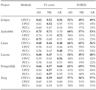
RQ3: How effective are CPCC+, CPCC, and PCC+ when dif-ferent underlying classifiers are used?
We find that CPCC+ outperforms PCC+ in ADTree, Naive Bayes, and Logistic Regression. Also, CPCC+ with ADTree as the underly classifier achieves the best performance.
RQ4: How much time does it take for CPCC+ and CPCC to run?
We find that the model building and prediction time for CPCC+ and CPCC are reasonable. On average, CPCC+ and CPCC need about 4.449 and 4.200 s to train a model, and 0.011 and 0.010 s to predict the label of an instance using the model.
The main contributions of this paper are as follows:
1) We propose CPCC, which utilizes the advantages of multi-objective GAs to combine different developers’ change data. Based on CPCC, we propose CPCC+ to further im-prove the performance.
2) We compare our method with PCC+ on 6 large software projects. The experiment results show that our method can achieve significant improvement over PCC+.
The remainder of this paper is organized as follows. We de-scribe some preliminary materials on CC and a motivating ex-ample in Section II. We describe the high-level architecture of CPCC in Section III. We elaborate the CPCC approach de-tails in Section IV. We elaborate CPCC+ approach dede-tails in Section V. We present our experiment setup and results in Sec-tions VI and VII. We discuss additional points on the benefits and limitations of our approach in Section VIII. We present related work in Section IX. We conclude and mention future work in Section X.
II. PRELIMINARIES
In this section, we first introduce the basic concepts of CC in Section II-A. Next, we describe the feature used in this paper in Section II-B. Then, we present the usage scenario of our proposed tool in Section II-C. Finally, we present the motivation of building a compositional model in Section II-D.
A. Change Classification
CC aims to predict if a particular file involved in a com-mit (i.e., a change) is buggy or not. Traditional CC techniques typically follow the following steps.
1) Training Data Extraction: For each developer’s change, label it as buggy or clean by mining a project’s revision history and bug tracking system [7], [18]. Buggy change means the change contains bugs (one or more), while clean change means the change has no bug. To identify which change is buggy, we follow the methods proposed by previous works [7], [18]. We first identify bug-fixing changes from the commit logs by searching the commit logs with the keyword “fix.” We assume the lines which are modified in the bug-fixing changes are the locations of a bug. Next, we use the command git blame, which annotates each line in a source code file with the most recent change that modified that line. We then intersect the locations of the bug with the git blame annotations to find the bug-introducing changes (aka., buggy changes). 2) Feature Extraction: Extract the values of various features
from each change. Many different features have been used in past CC studies.
3) Model Learning: Build a model by using a classifica-tion algorithm based on the labeled changes and their corresponding features. In this paper, by default, we use ADTree [19] to construct the prediction model.
4) Model Application: For a new change, extract the values of various metrics. Input these values to the learned model to predict whether the change is buggy or clean.
PCC modifies the above process by constructing not only one model during the model learning step, but rather a number of personalized models each trained using a developer historical data. In this work, similar to PCC, we still create multiple mod-els each for a particular developer. However, each model is now a collective one and takes into consideration not only the devel-oper historical data, but also the historical data of other relevant developers.
B. Features
In this paper, we consider three types of features, i.e., charac-teristic vector, word vector, and metadata. These features were used by Jiang, Tan, and Kim in their PCC work [7].
1) Characteristic Vector: A characteristic vector stores the number of times each node type appears in the abstract syntax tree (AST) of a code. Given a change, we build two characteristic vectors: one for the source code file before the change and one for the source code file after the change. We take the difference in the characteristic vector of the code prior to the change and the code after the change. Each element in the characteristic vector is a feature. Notice that the number of features in the characteristic vector are large because there are a large number of nodes in the AST.
Figs. 1 and 2 present an example of source code before and after the change. Suppose we only use if, for, and while node types for characteristic vectors. The characteristic vector of the code shown in Fig. 1 is0,2,0. And the characteristic vector
Fig. 1. Example of source code before the change.
Fig. 2. Example of source code after the change.
of the code shown in Fig. 2 is1,2,0. We then subtract the two characteristic vectors to obtain the difference, i.e., the difference for the code before and after the change is1,0,0.
2) Word Vector: Multiset of word tokens that appear in the commit message and source code of a change. Each word token in the multiset is a feature. We use the Snowball2 stemmer in
Weka to convert the strings into word vectors and represent them as the form of bags of words. Notice that the number of word features are large due to the large number of terms in the commit message.
3) Metadata: In addition to characteristic vector and word vector, we also use a number of metadata features: commit hour (0, 1, 2,. . ., 23), commit day, cumulative change count, cumulative buggy change count, source code file/path names, and file age (in days).
C. Usage Scenario
In this paper, we aim to build a prediction tool which identifies the buggy changes early on. The goal is to highlight defect-prone changes to improve the quality of source code. In practice, due to limited time budget and tight project schedule, developers are likely to inspect only a limited number of potentially buggy LOC to identify defect-prone changes. In such a case, it is crucial that manually inspecting the top percentages of lines that are likely to be buggy can help developers discover as many bugs as possible. The following scenarios illustrate the benefits of our tool. Scenario 1—Without Tool: Xin joins a new software project team as a developer. The release date for the project is approaching, so the project manager asks Xin to inspect the code to identify as many buggy code as possible. One problem for Xin is that he does not know where to begin to inspect the code, and he decides to inspect the code from the first file to the last file in the project. When Xin has inspected just about 20% of the source code, the project needs to be released. Xin only finds 20 bugs, and 180 bugs remain in the released product. Most customers encounter many bugs when using various features of the product and are extremely unhappy.
Scenario 2—With Tool: Xin joins a new software project team as a developer. The release date for the project is approaching, so the project manager asks Xin to inspect the code to identify as many buggy code as possible. Xin first mines historical data from git, uses our tool to identify likely buggy changes, ranks
TABLE I
F1-SCORE ANDCOSTEFFECTIVENESS(NOFB20) SCORES OFVARIOUSMODELS FOR THETWOTARGETDEVELOPERS(DEV1ANDDEV2) FROMECLIPSEJDT
Models Target Dev 1 Target Dev 2
F1-score NofB20 F1-score NofB20
P 0.55 44 0.63 39 O1 0.48 23 0.60 33 O2 0.43 61 0.46 33 O3 0.29 25 0.49 46 O4 0.19 35 0.28 26 O5 0.49 38 0.26 32 O6 0.13 40 0.26 29 O7 0.26 56 0.14 24 O8 0.26 51 0 14 All 0.54 35 0.43 26
The first row corresponds to the performance of the model built using the target developer’s own change data. The remaining nine rows corresponds to the performance of the model built using the remaining eight developers’ change data.
the changes from high to low confidence scores, and inspects the code in the changes one by one. When Xin inspects about 20% of the source code, the project needs to be released. Xin finds 180 bugs, and 20 remains in the released product. Only a minority of the customers encounter one or a few bug when using several features of the product, and only a few are mildly unhappy. D. Motivating Example
The effectiveness of our collective personalized CC technique relies on one primary hypothesis:
A model built from a relevant developer’s historical data can poten-tially be used to predict buggy changes of a target developer.
Here, we try to validate this hypothesis. To do so, we select ten developers from Eclipse JDT. We pick two developers as tar-get developers (Dev 1 and Dev 2), and we investigate whether a personalized model learned from each of the remaining eight developers (we refer them as source developers) can be used to predict buggy changes made by the target developers. We use ADTree to learn models from each of the eight developers—we denote these models asO1, O2, . . . , O8. We also combine all
of the eight developers’ data to train a global modelAll. Next, we use the same algorithm to learn a model from the target developer own data—we denote this model asP. We then test the models on the changes made by Dev 1 and Dev 2, and we measure the quality of these models by computing F1-score and cost effectiveness using tenfold cross-validation setup. More specifically, for each target developer, we divide the change data of the target developer into ten equal-sized folds, and we choose nine folds of the data to train a classifier and eval-uate the performance of a model in the remaining fold; the above process iterates ten times and the aggregate scores across the ten iterations are reported.
Table I presents the F1-score and cost effectiveness (NofB20) of various models for the two target developers. We notice that the global modelAlldoes not perform well; its NofB20 scores are lower than the other models. For Dev 1, the F1-score and NofB20 are 0.55 and 44, respectively, when the model built
using his/her own change data (i.e., P) is used. Interestingly, we notice that other models can achieve similar or even better performance thanP. In particular, using modelO2, the F1-score
and cost effectiveness are 0.43 and 61, respectively. Notice that O2’s cost effectiveness score is even higher than that of the
target classifier. For Dev 2, we also observe a similar result. For example, when O3 is used the cost effectiveness score is 46,
which is higher than that of the target classifierP. Thus, if we find a way to better use other developer data, the performance of CC can potentially be further improved.
From Table I, we also notice that the same model (i.e.,O1–O8)
has different performance when evaluated on different target developers’ change data. For example, the F1-score and cost effectiveness forO3 are 0.29 and 25 when evaluated on target
developer 1’s change data, which are lower than many other models. We note that the F1-score and cost effectiveness for O8 are 0 and 14, respectively, when it is evaluated on target
developer 2’s change data, which are much lower than the other models. We manually check the results, and we find that when we build a prediction model by using developer 8’s change data, it will predict all the changes in the target developer 2’s change data as clean C since it could not identify any true positive, its precision, recall, and F1-score are all zeroes. However, the same classifier could achieve F1-score and cost effectiveness of up to 0.49 and 46 when evaluates on target developer 2’s change data, which are higher than many other models. We refer to this phenomenon as target difference.
Moreover, in Table I, we notice that even for the same target developer, different models exhibit different performance. For example, for target developer 1,O2,O7, andO8 achieve much
better cost effectiveness scores than the remaining models. For target developer 2,O1,O2,O3, andO5achieve much better cost
effectiveness scores than the remaining models. We refer to this phenomenon as source difference.
We also check the F1-score and cost effectiveness for the other eight developers by using the same setting as we do for the target developers 1 and 2. And we find the phenomenon of target difference and source difference still exist. For example, when we predict the buggy changes for developer 4, we find the prediction model built on developer 2’s change data (i.e.,O2)
shows good performance, i.e., it achieves an F1-score and cost effectiveness of 0.54 and 57, respectively. But the prediction model built on developer 5’s change data (i.e.,O5) shows bad
performance, i.e., it achieves an F1-score and cost effectiveness of 0.21 and 27, respectively. Also, when we predict the buggy changes for developer 4, prediction models built on developer 1, 2, or 6’s change data (i.e., O1, O2, or O6) achieve much
better performance than the other models. And when we predict the buggy changes for developer 7, prediction models built on developer 3 or 8’s change data (i.e.,O3 or O8) achieve much
better performance than the other models.
Due to the phenomenon of target difference and source differ-ence, typically no single model always perform best on different target developers’ change data. Thus, a collective model which utilizes the advantages of different models can help to reduce the effect of target difference and source difference and fur-ther improve the performance of personalized defect prediction.
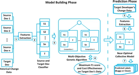
Fig. 3. Overall architecture of CPCC.
To achieve this goal, in this paper, we build a collective model using our proposed technique CPCC.
III. CPCC ARCHITECTURE
Fig. 3 presents the architecture of our CPCC framework. CPCC contains two phases: model building phase and prediction phase. In the model building phase, CPCC builds a collective model for each target developer, which is learned from historical change data of source developers and the target developer. In the prediction phase, we apply this model to predict if each of the target developer’s new changes is defective or not.
Our framework takes as input historical changes from various source developers and the target developer with known labels (i.e., buggy or clean). Next, it extracts the values of various features from these changes (Step 1). In this paper, we use the features as shown in Section II-B. These features were also previously used by Jiang, Tan, and Kim for PCC+ [7]. Then, our framework builds multiple personalized prediction models based on the extracted feature values (Step 2). In total, we have
(n+ 1) prediction models, where the firstnmodels are built from the source developers’ changes, and the final model is built from the target developer’s changes. Next, CPCC searches for the near-optimal composition of these models by leveraging a multiobjective GA (Step 3). The algorithm picks a composite (or collective) model that maximizes F1-score and cost effec-tiveness (NofB20) when it is used to predict the labels of the target developer’s historical changes (Step 4). The near-optimal composition model is a machine learning classifier which as-signs labels (in our case: buggy or clean) to a change based on its feature values.
After the model is constructed, in the prediction step, it is then used to predict whether each of the target developer’s new changes is defective or not. For each new change, we first extract the values of the same set of features as those considered in the model building step (Step 5). We then input the values of these features into the learned model (Step 6). It will output a prediction result which is one of the following labels: buggy or clean (Step 7).
IV. CPCC APPROACH
In this section, we elaborate how CPCC builds a collective model for a target developer in a software project which corre-sponds to Steps 2–4 in Fig. 3. We also elaborate how the model can be used to predict if an unknown change is buggy or clean (Step 5 in Fig. 3).
Assumingnsource developers (i.e., other developers in the project), CPCC first builds a total of(n+ 1)prediction models (or classifiers3): for a source developer Dev
i,{1≤i≤n}, it
builds a modelSi from his/her historical change data; for the
target developerT arget, it builds the(n+ 1)th modelT from T arget’s historical change data. CPCC then searches for a near-optimal collective model containing these(n+ 1)models along with a set of weights and a threshold to decide if a change is buggy or not. We refer to this collective model as the CPCC classifier. A multiobjective GA is used to learn the best values for these weights and the threshold. It will search for a solution (i.e., a collective model) in a search space based on a set of objective functions. The best solution is then outputted.
In Section IV-A, we formally define the CPCC classifier and how it can be used to predict if a change is clean or buggy. We formally present the search space of all possible combina-tions of n+ 1 classifiers to construct the CPCC classifier in Section IV-B. Section IV-B also introduces the objective func-tions. We elaborate the detailed procedure of how multiobjective GA is used to learn the CPCC classifier in Section IV-C. A. CPCC Classifier
A CPCC classifier integrates the n+ 1 prediction models (classifiers):S1, . . . , Sn andT. Given a changej, a modelSi
outputs a confidence score that indicates the likelihood ofjto be buggy, which is denoted as Scorei(j). Similarly, we denote the
confidence score of the target classifierTtojas Scoret(j). The
range of a confidence score is from 0 to 1. A CPCC classifier computes a weighted sum of all confidence scores assigned by
the(n+ 1) classifiers and predicts whetherj is buggy or not based on a threshold score. Definition 1 provides a mathematical definition of the CPCC classifier.
Definition 1 (CPCC Classifier): Consider n source classi-fiers{S1, S2, . . . , Sn}and a target classifierT. A CPCC
clas-sifier composes these(n+ 1)classifiers and assigns a label to an instancej, denoted as Label(j), as follows:
Label(j) = 1(i.e., buggy), 0(i.e., clean), if CP CC(j)≥threshold Otherwise where CPCC(j) = n i= 1αi×Scorei(j) +αt×Scoret(j) LOC(j) . (1)
In the above equation, Scorei(j)is the confidence score
out-putted by theith source classifier for instance j to be buggy, α1–αn are the weights of the n source classifiers, Scoret(j)
is the confidence score outputted by the target classifierT for instancejto be buggy,αt is the weight of the target classifier,
threshold is the boundary used to decide whether an instance is buggy or not, and LOC(j)is the number of LOCs for in-stance j. CPCC(j) is the composite confidence score for in-stancej to be buggy, and we set it as a linear combination of the confidence scores outputted by thensource classifiers and the target classifier T. Instancej is classified as buggy if its composite confidence score CPCC(j)is larger than or equal to threshold; otherwise, it is classified as clean. Note thatα1–αn,
αt, and threshold are the parameters of a CPCC classifier. Thus,
we denote a CPCC classifier as (i= 1n{(αi, Si)},(αt, T),
threshold), where eachSiis a source classifier,αiis the weight
ofSi,Tis a target classifier,αtis the weight ofT, and threshold
is the defect boundary.
We include LOC in (1) to maximize the number of buggy changes found given a budget (e.g., inspecting only 20% of the number of LOC). If two changes have equal likelihood to be buggy and one of them has a higher LOC, to find as many bugs as possible within the budget, we need to pick the change with the lower LOC.
Note that the CPCC score may be larger than 1—since the numerator of formula (1) may be larger than 1, and the denom-inator of formula (1) may be equal to 1. This may make the output of CPCC noninterpretable since the range of values that it can take is very large. Still, since the CPCC score is only an intermediary score, we believe it is okay for the score to be noninterpretable. If an interpretable score is needed, we can normalize the output of the CPCC formula by dividing it with the sum of the weights (i.e.,α1+· · ·+αn+αt). If we also
normalize the threshold in the same way, this modification will not affect the inferred labels.
Example: Consider a changejwhich has 100 LOCs. Suppose we have three source classifiers and one target classifier. Let the confidence scores of the three source classifiers and the target classifier forjbe0.4,0.5,0.8, and0.9, respectively. Also, let the weights of the source classifiers and the target classifiers be 0.3, 0.7, 0.7, and 0.8, respectively. From the above, the composite
confidence score forjis
0.3×0.4 + 0.7×0.5 + 0.7×0.8 + 0.8×0.9
100 = 0.0175.
If the bug boundary is less than or equal to 0.0175, then CPCC predictsjas buggy, else it predicts it as clean.
B. Search Space and Objective Functions
1) Search Space: The search space of all possible compo-sitions corresponds to the various assignments of values to the weightsα1, α2, . . . , αn of the source classifiers, the weightαt
of the target classifier, and the bug boundary threshold. Each weight is a real number from zero to one and threshold is a positive real number. We refer to each composition as a solu-tion in the search space, and it comprises of a set of parameters Par={α1, α2, . . . , αn, αt,threshold}.
2) Objective Functions: An objective function measures the quality of a solution in a search space. We have two objective functions that we try to maximize:
F1(Par)
cost(Par). (2)
In the above equation, F1(Par) and cost(Par) are the F1-score and the cost effectiveness (NofB20) achieved by a CPCC classifier with parameters Par on a training data. The details on how F1-score and cost effectiveness are computed are given in Section VI-C. Notice that we choose the objective functions as F1 and cost effectiveness, since these two evaluation metrics are widely used in defect prediction literature [1], [8]–[12], [16], [17], and we would like our constructed model to not only achieve good F1-score but also have good cost effectiveness score.
Since we have two different objective functions to be maxi-mized, we find a set of Pareto optimal solutions (cf., [17], [20]) defined in Definition 2.
Definition 2 (Dominance and Pareto optimal solutions): A set of parameters Paridominates another set of parameters Parj
if and only if the values of the two objective functions (i.e., F1-score and cost effectiveness) satisfy
F1(Pari)>F1(Parj)and cost(Pari)≥cost(Parj)
or
F1(Pari)≥F1(Parj)and cost(Pari)>cost(Parj).
A set of parameters Pari is Pareto optimal if and only if no
other set of parameters dominates it in the feasible region, i.e., no other set of parameters Parj exists that would improve the
F1-score, without worsening cost effectiveness scores, and vice versa.
There would be a number of solutions which are Pareto opti-mal. We further reduce these solutions by selecting the following subset
ParSetselected= argmax Pari∈Pareto
F1(Pari)×cost(Pari). (3)
In other words, we select solutions from the Pareto optimal set which has the highest product of F1-score and cost effectiveness
scores. We randomly pick a solution from this set as the near-optimal solution.
C. Detailed Procedure
We employ a multiobjective GA [20] to learn the weights (α1–αn andαt) and the threshold (threshold). In the
multiob-jective GA, solutions in a search space are modeled as chro-mosomes. A chromosome contains a set of genes where a gene corresponds to a part of a solution (i.e., a value of a weight, or a value of the threshold, in our setting). The multiobjective GA begins with an initial set of random chromosomes, referred to as the initial population. Next, the population evolves in a num-ber of iterations, and in each iteration, it generates subsequent generations, where each generation is a population of chromo-somes. To create the next generation, multiobjective GA will do three operations: selection, crossover, and mutation. Selection operation refers to the process that selects parent chromosomes according to their objective function scores (F1-score and cost effectiveness); thus, the parent chromosomes that have high ob-jective function scores have high probability to survive in the next generation. Crossover operation refers to the process that merges the genes of two parent chromosomes to form offspring chromosomes according to a given probability. Mutation refers to the process that the genes of offspring chromosomes would be modified according to a given probability. More details about multiobjective GA can be found in [20].
There are many variants of the multiobjective GA; in this pa-per, we use an algorithm named vNSGA-II, which is proposed by Deb, Pratap, Agarwal, and Meyarivan [21]. In our setting, each chromosome is represented as an array of(n+ 2)double;
(n+ 1)double represent the weights (α1–αn andαt), and the
last double represents the threshold. We use the Roulette wheel selection procedure [22], [23] as the selection operator. It as-signs a high probability to a chromosome with higher objective function scores. For the crossover operator, we use the simu-lated binary crossover (SBX) operator [24]. For the mutation operator, we use the polynomial mutation (PM) operator [25]. SBX and PM attempt to simulate the offspring distribution of binary-encoded bit-flip crossover and mutation on real-valued variables, respectively.
Algorithm 1 presents the detailed steps to train a CPCC clas-sifier. For theith source developer’s historical dataDi, we first
build a classifierSibased on instances inDi(lines 9–11).
Sim-ilarly, we build a classifierT using the target developer’s data Dt alone (line 12). Then, we create an initial population (i.e.,
P) containing PopSize chromosomes (i.e., solutions) that are chosen randomly, and we record the set of nondominated solu-tions (i.e., the solusolu-tions with nondominated F1-score and cost effectiveness scores onDt) among the solutions inP (lines 13
and 14). Remember that each solution inP is a set of weights
{α1, α2, . . . , αn},αt, and a threshold. Next, we evolve the
pop-ulation in MaxGen iterations; for each iteration, we perform the selection, crossover, and mutation operations on the current population and record the set of nondominated solutions so far (lines 16–22). After the iterations complete, we find the set of Pareto optimal solutions from the set of nondominated solutions
Algorithm 1: The Model Building Phase of CPCC. 1: CPCC({D1, D2, . . . , Dn},Dt, PopSize, MaxGen)
2: Input:
3: {D1, D2, . . . , Dn}: Historical data of source
developers
4: Dt: Historical data of the target developer
5: P opSize: Number of chromosomes in a population 6: M axGen: Maximum number of generations
7: Output: Composite CPCC Classifier (ni= 1αiSi,αtT,
threshold). 8: Method:
9: for allDi⊆ {D1, D2, . . . , Dn}do
10: Build a classifierSiby usingith source developer’s
historical data; 11: end for
12: Build a classifierT by using the target developer’s historical dataDt;
13: LetP=Initial population withP opSizemembers; 14: EvaluatePand record the set of nondominated
solutions (i.e., the solutions with nondominated F1-score and cost effectiveness scores onDt) so far;
15: LetcurGen=0
16: whilecurGen < M axGendo 17: LetP =select(P); 18: P =crossover(P); 19: P =mutation(P);
20: EvaluateP and record the set of non dominated solutions so far;
21: curGen=curGen+ 1; 22: end while
23: Find the set of Pareto optimal solutions;
24: Output (ni= 1αiSi,αtT,threshold) which achieves
the highest product of F1-score and cost effectiveness scores in the set of Pareto optimal solutions.
(line 23). The algorithm returns a set ofα1, α2, . . . , αn,αt, and
threshold values, which achieves the highest product of F1-score and cost effectiveness in the set of Pareto optimal solutions. If there are more than one of such near-optimal set, we randomly pick one of them.
D. Complexity Analysis
In our CPCC, we use a multiobjective GA (i.e., vNSGA-II [20], [26]–[28]) to find good values of some parameters (i.e., the weights and the threshold), and we use ADTree [19] as the default underlying classifier. Suppose we haveM objective functions and a population size ofN; then, the time complex-ity of vNSGA-II isO(M ×N2). Suppose our dataset haveP
features, and Qnumber of instances, the time complexity of ADTree [19] isO(P×Q2). Thus, the total time complexity of
CPCC isO(M×N2+P×Q2).
V. CPCC+: A COMPOSITEAPPROACH
To further improve classification performance, we propose CPCC+ which combines CPCC and PCC. Similar to CPCC,
CPCC+ also has two phases: model building phase and pre-diction phase. In the model building phase, for each target de-veloper, CPCC+ builds a prediction model using CPCC and another one using PCC. In the prediction phase, for a new un-labeled change, CPCC+ predicts the change as clean or buggy using the two prediction models built in the model building phase. It first obtains the confidence scores of an instance to be buggy that are outputted by the two prediction models. It then normalizes the scores produced by CPCC and PCC so that their scores are comparable. It does this by adjusting the CPCC confidence score for instancejto be buggy as follows:
CPCCAdj(j) = CPCC(j)
CPCC(j) +threshold. (4) Note that we only normalize the CPCC scores [using (4)]. We do not normalize the PCC scores since they are already normalized. They are probabilities outputted by a classification algorithm and their scores are already between zero and one. For CPCC scores, they can be larger than one, and thus, we normalize them.
Next, based on the adjusted CPCC confidence score and the PCC confidence score, it chooses the prediction with the highest confidence as the final prediction.
More formally, for a new change, new, let us denote the larger of CPCCAdj’s and PCC’s confidence of new to be buggy
as Scoremaxbuggy(new), and the larger of CPCCAdj’s and PCC’s
confidence of new to be clean4 as Scoremax
clean(new). Based on
these notations, CPCC+ assigns a label to new as follows: Label(new) = 1(i.e., buggy), 0(i.e., clean), if CPCC+(new)≥0 Otherwise where CPCC+(new)= Score max
buggy(new)−Scoremaxclean(new)
LOC(new) . (5)
In the above equation, CPCC+ (new) is CPCC+’s confi-dence that new is buggy, and LOC(new)is the number of LOCs in change new. The LOC does not determine if a change is predicted as buggy or not. We use LOC to help rank the pre-dicted buggy changes. For two changes with similar likelihood to be buggy, we will rank the one with less LOC first so as to maximize the number of bugs found given an inspection budget. A. Complexity Analysis
As shown in Section IV-D, the total time complexity of CPCC isO(M ×N2+P×Q2). In CPCC+, we combine CPCC and
PCC. Suppose our dataset have P features and Qnumber of instances, the time complexity of PCC using ADTree isO(P× Q2). Thus, the total time complexity of CPCC+ is O(M ×
N2 +P×Q2).
4The confidence of new to be clean is one minus the confidence of new to be
buggy.
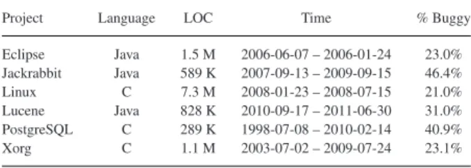
TABLE II
STATISTICS OFCOLLECTEDDATA
Project Language LOC Time % Buggy
Eclipse Java 1.5 M 2006-06-07 – 2006-01-24 23.0% Jackrabbit Java 589 K 2007-09-13 – 2009-09-15 46.4% Linux C 7.3 M 2008-01-23 – 2008-07-15 21.0% Lucene Java 828 K 2010-09-17 – 2011-06-30 31.0% PostgreSQL C 289 K 1998-07-08 – 2010-02-14 40.9% Xorg C 1.1 M 2003-07-02 – 2009-07-24 23.1%
VI. EXPERIMENTSETUP
In this section, we describe the settings that we follow to evaluate the effectiveness of our proposed CPCC and CPCC+. We first present our dataset, cross-validation settings, and ex-perimental environment. We then present our parameter setting and evaluation metrics.
A. Datasets, Cross-Validation Settings, and Environment We use the same datasets as Jiang, Tan, and Kim [7], which contain changes from six open-source software projects: Eclipse JDT, Jackrabbit, Linux, Lucene, PostgreSQL, and Xorg. Table II presents the statistics of Jiang, Tan, and Kim’s data. The columns correspond to the programming language (Language), LOCs (LOC), the time period of collected changes (Time), and the percentage of buggy changes (% Buggy Changes). Jiang, Tan, and Kim selected top ten developers from each project. For each of them, they collected 100 consecutive changes from the time period listed in Table II. Thus, in total, there are 1000 changes for each project.
Jiang, Tan, and Kim have shown that PCC+ outperforms CC, PCC, and weighted PCC; thus, in this work, since we use the same dataset, we only need to compare our technique CPCC+ and CPCC with PCC+. We perform tenfold cross validation 100 times and take the average performance to reduce the training set selection bias. For each tenfold cross validation, we randomly split the data into ten subsets. The random splitting is performed differently for each of the tenfold cross validations. Cross vali-dation is a standard evaluation setting, which is widely used in software engineering studies; cf., [1], [4], [7], [9], [29]–[32].
Note that our CPCC+ and CPCC use a multiobjective GA (i.e., vNSGA-II) to optimize the values of some parameters (e.g., the weights and the threshold). To do this step, we cre-ate a validation set from a training data. For each training fold and each target developerj, we separatej’s change data in the training data of that fold to create a validation set. Next, we use the multiobjective GA to optimize the parameters for this validation set. Furthermore, since multiobjective GA exhibits some randomness [20], [21], for each of the 100 tenfold cross validations, we run the multiobjective GA ten times and use the average performance score. This follows the recommenda-tion made by Liu, Khoshgoftaar, and Seliya [33] and Canfora et al. [17] to evaluate random algorithms in software engineer-ing context. PCC+ is a deterministic algorithm and thus there is no need to perform these repetitions.
The experimental environment is a Windows 8, 64-bit, Intel(R) Core(TM) 1.60-GHz laptop with 4-GB RAM.
B. Parameter Setting
Our multiobjective GA vNSGA-II [34] accepts some param-eters. The parameters of vNSGA-II that we use in this study are as follows.
1) Population size: We set a moderate population size with PopSize= 200.
2) Number of generations: We set the maximum number of generations MaxGen= 1000.
3) Crossover operator: We use an SBX operator with prob-abilitypc= 0.6.
4) Mutation operator: We use a PM operator with probability pm = 0.05.
CPCC+, CPCC, and PCC+ use an underlying classifier. By default, we use the same classifier that was used by Jiang, Tan, and Kim to evaluate PCC+ [7], namely ADTree [19]. We use the implementation of ADTree that comes with Weka [35]. C. Evaluation Metrics
We use two evaluation metrics: cost effectiveness and F1-score. These two measures are useful in different situations. Cost effectiveness is useful when there are limited resources to inspect a limited amount of code due to a hectic schedule of development. F1-score is useful when there is sufficient resource to inspect all of the predicted buggy changes.
1) Cost Effectiveness: Cost effectiveness is a widely used evaluation metric for defect prediction [7]–[12], which evaluates prediction performance given a cost limit. In our setting, the cost is the LOC to inspect. We use the same cost effectiveness setup as the one used by Jiang, Tan, and Kim [7]. They measure the number of buggy changes that a developer can identify by inspecting the top 20% LOC with the highest confidence to be buggy. They refer to this number as NofB20. Consider different projects have different numbers of bugs; we also compute a percentage of the total number of bugs (PofB20) by normalizing the NofB20 scores .
To compute NofB20 and PofB20, we sort changes in the test data based on the confidence levels that a CC technique outputs for each of them. A change with a higher confidence level is deemed to be more likely to be buggy by the CC technique. We then simulate a developer that inspects these potentially buggy changes one at a time. As the changes are inspected one at a time, we accumulate the number of LOC that are inspected and the number of buggy changes identified. We stop the process when 20% of the LOC have been inspected and output the number of buggy changes that are identified. This number is the NofB20 score. A higher cost effectiveness score represents that a developer can detect more bugs when inspecting a limited number of LOC.
2) F1-Score: There are four possible outcomes for a change in the test data: A change can be classified as buggy when it truly is buggy (true positive, TP); it can be classified as buggy when it is actually clean (false positive, FP); it can be classified as clean when it is actually buggy (false negative, FN); or it
can be classified as clean and it truly is clean (true negative, TN). Based on these possible outcomes, precision, recall and F1-score are defined as follows.
Precision: The proportion of changes that are correctly la-beled as buggy among those lala-beled as buggy:
P =TP/(TP+FP). (6) Recall: The proportion of buggy changes that are correctly labeled:
R=TP/(TP+FN). (7) F1-score: A summary measure that combines both precision and recall—it evaluates if an increase in precision (recall) outweighs a reduction in recall (precision):
F = (2×P×R)/(P+R). (8) There is a tradeoff between precision and recall. One can increase precision by sacrificing recall (and vice versa). In our framework, we can sacrifice precision (recall) to increase recall (precision), by manually lowering (increasing) the value of the threshold parameter in Definition 1. The tradeoff causes difficul-ties to compare the performance of several prediction models by using only precision or recall alone [36]. For this reason, we compare the prediction results using F1-score, which is a harmonic mean of precision and recall. This follows the setting used in many CC and defect prediction studies [1], [7], [16] and various software analytics studies [37], [38].
VII. EXPERIMENTRESULTS
In this section, we present our experiment results which an-swer a number of research questions. We present these questions and their answers in the following subsections.
A. RQ1: How Effective is CPCC+ and CPCC? How Much Improvement Can They Achieve Over the State-of-the-Art Method?
Motivation: We need to compare CPCC+ and CPCC with the state-of-the-art CC method. Answer to this research question would shed light to the extent CPCC+ and CPCC advances the state of the art.
Approach: In a recent work, Jiang, Tan, and Kim have demon-strated that PCC+ outperforms a number of other CC meth-ods [7]. Thus, to answer this research question, we compare CPCC+ and CPCC with PCC+ and CC. We compute NofB20, PofB20, and F1-score to evaluate the performance of these two approaches on the six projects. Also, in this paper, we use 100 times tenfold cross validation to evaluate each of the methods, and for each approach (i.e., CPCC+, CPCC, PCC+, and CC), at the end of each of the tenfold cross validation, it will out-put an F1 and PofB20 score. We apply Wilcoxon signed-rank test [40] on the 100 paired data to test whether the improve-ment of CPCC+ and CPCC over PCC+ and CC is significant. We also use Bonferroni correction [41] to counteract the results of multiple comparisons. We consider that the improvement is statistically significant if the p-value is less than 0.05 (i.e., at the confidence level of 95%) after Bonferroni correction.
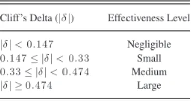
TABLE III
CLIFF’SDELTA ANDTHEEFFECTIVENESSLEVEL [9]
Cliff’s Delta (|δ|) Effectiveness Level
|δ|<0.147 Negligible
0.147≤ |δ|<0.33 Small
0.33≤ |δ|<0.474 Medium
|δ| ≥0.474 Large
We also use Cliff’s delta (δ) [39], which is a nonparametric effect size measure that quantifies the amount of difference be-tween two groups. In our context, we use Cliff’s delta to compare CPCC+ and CPCC to the baseline approaches. For example, when compared the F1-score of CPCC+ with PCC+, the two groups are the F1-scores of CPCC+ and PCC+. The delta values range from−1 to 1, whereδ=−1or1indicates the absence of overlap between two approaches (i.e., all values of one group are higher than the values of the other group, and vice versa), whileδ= 0indicates that the two approaches are completely overlapping. Table III describes the meaning of different Cliff’s delta values and their corresponding effectiveness level [39]. Notice that different from Wilcoxon signed-rank test which is used to test whether the improvements of CPCC+ and CPCC over the baseline approaches are statistically significant, Cliff’s delta is used to test whether the improvements of CPCC+ and CPCC over the baseline approaches are of substantially large amount. If the effect size is medium or large, we consider the improvement to be substantial.
Results: Table IV presents the experiment results comparing CPCC+ and CPCC with PCC+ and CC. The experiment results are a little different than what were reported in [7]. This is the case as the tenfold cross validation used in our experiments randomly partitions the dataset into ten sets. Due to the random-ness in the process, the resultant sets are different than those produced by the random partitioning performed in Jiang, Tan, and Kim’s experiments. Also, differently from Jiang, Tan, and Kim’s experiment setup, we run tenfold cross validation 100 times and record the average experiment results.
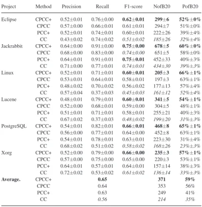
From Table IV, we can note that the F1, NofB20, and PofB20 scores of CPCC vary from 0.58 to 0.74, 197 to 651, and 48% to 63%, respectively. On average, across the six projects, CPCC can achieve F1, NofB20, and PofB20 scores of 0.64, 353, and 56%, respectively. In terms of NofB20, CPCC improves PCC+ and CC by 20–229 and 34–284, respectively. In terms of PofB20, CPCC improves PCC+ and CC by 6–32% and 11–40%, respec-tively. In terms of F1 score, CPCC improves PCC+ and CC by 0.01–0.02 and 0.00–0.13, respectively. On average, CPCC im-proves PCC+ in terms of NofB20, PofB20, and F1 score by 104, 15%, and 0.01 and improves CC in terms of NofB20, PofB20, and F1 score by 139, 21%, and 0.08, respectively.
We also notice that the F1, NofB20, and PofB20 scores of CPCC+ vary from 0.60 to 0.75, 205 to 678, 52% to 66%, respec-tively. On average, across the six projects, CPCC can achieve F1, NofB20, and PofB20 scores of 0.65, 371, and 59%, respectively. In terms of NofB20, CPCC+ improves CPCC, PCC+, and CC by 5–37, 20–229, and 44–300, respectively. In terms of PofB20,
CPCC+ improves CPCC, PCC+, and CC by 1–4%, 9–34%, and 14–42%, respectively. In terms of F1 score, CPCC+ improves CPCC, PCC+, and CC by 0.01–0.02, 0.02–0.04, and 0.01–0.15, respectively. On average, CPCC+ improves PCC+ in terms of NofB20, PofB20, and F1 score by 122, 24%, and 0.02, respec-tively, and improves CC in terms of NofB20, PofB20, and F1 score by 157, 24%, and 0.09, respectively. Moreover, we notice that for NofB20 and PofB20, the performance gap between CC and PCC+ is smaller than the performance gap between CPCC+ and PCC+. On the other hand, for F1 score, the performance gap between CC and PCC+ is larger than the performance gap between CPCC+ and PCC+.
Moreover, we notice CPCC+ and CPCC are more stable than PCC+ and CC. From Table IV, we notice that the standard deviations for CPCC+ and CPCC are from 0.00 to 0.01 and 0% to 1% in terms of F1 and PofB20 scores, while these values for PCC+ and CC are from 0.01 to 0.03 and 3% to 4% in terms of F1 and PofB20 scores, respectively.
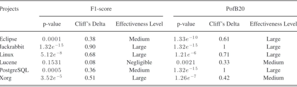
To investigate whether the improvements of CPCC+ over CPCC, PCC+, and CC are statistically significant and the effec-tive sizes are large, we also compute the p-value in Wilcoxon signed-rank test and Cliff’s Delta. Table V presents the p-values and Cliff’s delta of comparing CPCC+ results with those of PCC+. Notice that in our study, we use Bonferroni correction to counteract the results of multiple comparisons; thus, the p-values are adjusted. We notice that the improvements of CPCC+ over PCC+ are statistically significant on all of the six projects in terms of F1-score and PofB20 at the 95% confidence level. Moreover, the effect sizes are mostly large.
Table VI presents the p-values and Cliff’s delta of comparing CPCC+ results with those of CC. The p-values are adjusted by using Bonferroni correction. We notice that the improvements of CPCC+ over CC are statistically significant on all of the six projects in terms of F1-score and PofB20 at the 95% confidence level. Moreover, the effect sizes are mostly large.
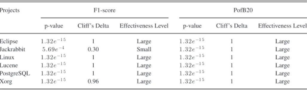
Table VII presents the p-values and Cliff’s delta of compar-ing CPCC+ results with those of CPCC. The p-values are ad-justed by using Bonferroni correction. We notice that in terms of PofB20, the improvements of CPCC+ over CPCC are statis-tically significant at 95% confidence level. In terms of F1-score, except for project Eclipse, CPCC+ statistically significantly out-performs CPCC. Moreover, the effect sizes are mostly large.
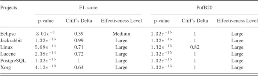
Table VIII presents the p-values and Cliff’s delta of com-paring CPCC results with those of PCC+. The p-values are adjusted by using Bonferroni correction. We notice that the im-provements of CPCC over PCC+ are statistically significant on all of the six projects in term of F1-score and PofB20 at the 95% confidence level. Moreover, the effect sizes are mostly large.
Table IX presents the p-values and Cliff’s delta of comparing CPCC results with those of CC. The p-values are adjusted by using Bonferroni correction. We notice that the improvements of CPCC over CC are statistically significant on all of the six projects in term of F1-score and PofB20 at the 95% confidence level. Moreover, the effect sizes are mostly large.
On average across the six projects, CPCC+ improves PCC+ by 0.02 and 122 in terms of F1 and NofB20 scores, respectively.
TABLE IV
EXPERIMENTRESULTS OFCPCC+ANDCPCC COMPAREDWITHPCC+ANDCC
Project Method Precision Recall F1-score NofB20 PofB20 Eclipse CPCC+ 0.52±0.01 0.76±0.00 0.62±0.01 299±6 52%±0% CPCC 0.57±0.00 0.66±0.01 0.61±0.01 294±7 51%±0% PCC+ 0.52±0.01 0.74±0.01 0.60±0.01 222±26 39%±4% CC 0.43±0.02 0.74±0.02 0.51±0.02 185±26 32%±4% Jackrabbit CPCC+ 0.64±0.00 0.91±0.00 0.75±0.00 678±5 60%±0% CPCC 0.68±0.00 0.83±0.00 0.74±0.00 651±5 58%±0% PCC+ 0.64±0.01 0.91±0.01 0.75±0.01 452±33 40%±3% CC 0.71±0.00 0.77±0.01 0.74±0.01 434±30 39%±3% Linux CPCC+ 0.52±0.01 0.71±0.01 0.60±0.01 205±3 66%±1% CPCC 0.53±0.01 0.64±0.01 0.58±0.01 197±3 63%±1% PCC+ 0.48±0.02 0.70±0.02 0.56±0.02 177±13 57%±4% CC 0.57±0.04 0.37±0.03 0.45±0.03 161±12 52%±4% Lucene CPCC+ 0.48±0.01 0.79±0.01 0.60±0.01 341±5 54%±1% CPCC 0.52±0.00 0.68±0.01 0.59±0.00 304±5 48%±1% PCC+ 0.51±0.01 0.71±0.01 0.58±0.01 255±21 40%±3% CC 0.67±0.02 0.37±0.03 0.48±0.02 199±20 31%±3% PostgreSQL CPCC+ 0.54±0.01 0.82±0.01 0.66±0.01 468±8 65%±1% CPCC 0.56±0.00 0.77±0.01 0.64±0.00 452±8 63%±1% PCC+ 0.54±0.01 0.78±0.01 0.63±0.01 223±30 31%±4% CC 0.68±0.02 0.51±0.02 0.58±0.02 168±26 23%±3% Xorg CPCC+ 0.52±0.00 0.79±0.00 0.66±0.00 235±3 57%±1% CPCC 0.57±0.00 0.75±0.00 0.65±0.00 220±3 53%±1% PCC+ 0.64±0.01 0.57±0.01 0.64±0.01 157±14 38%±3% CC 0.72±0.02 0.53±0.02 0.61±0.02 136±14 33%±3% Average. CPCC+ 0.65 371 59% CPCC 0.64 353 56% PCC+ 0.63 249 41% CC 0.56 214 35%
The results are in the form of mean±standard deviation (std). The highest and lowest results for each dataset are in bold and italic, respectively.
TABLE V
P-VALUE ANDCLIFF’SDELTA OFCOMPARINGCPCC+ RESULTSWITHTHOSE OFPCC+
Projects F1-score PofB20
p-value Cliff’s Delta Effectiveness Level p-value Cliff’s Delta Effectiveness Level
Eclipse 1.01e−5 0.37 Medium 1.32e−1 5 1 Large
Jackrabbit 1.32e−1 5 0.98 Large 1.32e−1 5 1 Large
Linux 5.10e−1 5 0.75 Large 5.10e−1 5 0.75 Large
Lucene 2.35e−1 3 0.76 Large 1.32e−1 5 1 Large
PostgreSQL 1.32e−1 5 1 Large 1.32e−1 5 1 Large
Xorg 5.84e−1 1 0.6014 Large 1.32e−1 5 1 Large
In most cases, the improvements are statistically significant and the effective sizes are large.
B. RQ2: How Effective Are CPCC+, CPCC, and PCC+ When Different Percentages and Number of LOC Are Inspected?
Motivation: By default, we set the percentage of LOC to inspect as 20%. In this RQ, we also investigate the performance of CPCC+, CPCC, and PCC+ when different percentages of LOC are inspected. Additionally, we also investigate the effectiveness of CPCC+, CPCC, and PCC+ when a fixed budget is specified, i.e., an absolute number of LOC to inspect. Answer to this research question can verify whether CPCC+ and CPCC still improve PCC+ for other cost settings.
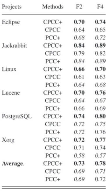
Approach: To answer this research question, we plot cost ef-fectiveness graphs that show the percentages of bugs that can be
detected by inspecting different percentages of LOC. Moreover, we also compute the area under the curve (AUC) in these graphs. In our graphs, we denote the percentage of LOC to inspect asp, and the PofB score as PofB; then, the AUC value is computed by
AUC=
PofB×p dp. (9)
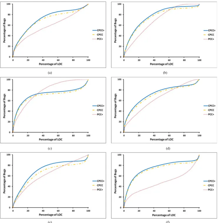
Results: Fig. 4 presents the cost effectiveness graphs for Eclipse JDT, Jackrabbit, Linux, Lucene, PostgreSQL, and Xorg. We can note that inspecting 20% of the LOC, CPCC+ could identify more than 50% of the defects in all of the six projects. We also notice that CPCC+ is better than PCC+ for a wide range of percentages of LOC to inspect. For Eclipse JDT and Xorg, the percentage range for which CPCC+ achieves the best performance are wide, i.e., from around 1% to 95%. For PostgreSQL, the percentage range for which CPCC+ achieves
TABLE VI
P-VALUE ANDCLIFF’SDELTA OFCOMPARINGCPCC+ RESULTSWITHTHOSE OFCC
Projects F1-score PofB20
p-value Cliff’s Delta Effectiveness Level p-value Cliff’s Delta Effectiveness Level
Eclipse 1.32e−1 5 1 Large 1.32e−1 5 1 Large
Jackrabbit 1.22e−1 2 0.66 Large 1.32e−1 5 1 Large
Linux 1.32e−1 5 1 Large 1.32e−1 5 1 Large
Lucene 1.32e−1 5 1 Large 1.32e−1 5 1 Large
PostgreSQL 1.32e−1 5 1 Large 1.32e−1 5 1 Large
Xorg 1.32e−1 5 0.96 Large 1.32e−1 5 1 Large
TABLE VII
P-VALUE ANDCLIFF’SDELTA OFCOMPARINGCPCC+ RESULTSWITHTHOSE OFCPCC
Projects F1-score PofB20
p-value Cliff’s Delta Effectiveness Level p-value Cliff’s Delta Effectiveness Level
Eclipse 1 0.11 Negligible 1.32e−1 5 1 Large
Jackrabbit 1.32e−1 5 0.85 Large 1.32e−1 5 1 Large
Linux 1.50e−6 0.31 Small 1.32e−1 5 1 Large
Lucene 1.32e−1 5 0.75 Large 1.32e−1 5 1 Large
PostgreSQL 1.32e−1 5 1 Large 1.32e−1 5 1 Large
Xorg 0.2852 0.15 Negligible 1.32e−1 5 1 Large
TABLE VIII
P-VALUE ANDCLIFF’SDELTA OFCOMPARINGCPCC RESULTSWITHTHOSE OFPCC+
Projects F1-score PofB20
p-value Cliff’s Delta Effectiveness Level p-value Cliff’s Delta Effectiveness Level
Eclipse 2.15e−6 0.39 Medium 1.32e−1 5 1 Large
Jackrabbit 1.2e−1 4 0.78 Large 1.32e−1 5 1 Large
Linux 4.73e−13 0.67 Large 1.32e−1 5 1 Large
Lucene 6.30e−6 0.40 Medium 1.32e−1 5 1 Large
PostgreSQL 1.32e−1 5 0.77 Large 1.32e−1 5 1 Large
Xorg 1.06e−9 0.55 Large 1.32e−1 5 1 Large
TABLE IX
P-VALUE ANDCLIFF’SDELTA OFCOMPARINGCPCC RESULTSWITHTHOSE OFCC
Projects F1-score PofB20
p-value Cliff’s Delta Effectiveness Level p-value Cliff’s Delta Effectiveness Level
Eclipse 1.32e−1 5 1 Large 1.32e−1 5 1 Large
Jackrabbit 5.69e−4 0.30 Small 1.32e−1 5 1 Large
Linux 1.32e−1 5 1 Large 1.32e−1 5 1 Large
Lucene 1.32e−1 5 1 Large 1.32e−1 5 1 Large
PostgreSQL 1.32e−1 5 1 Large 1.32e−1 5 1 Large
Xorg 1.32e−1 5 0.96 Large 1.32e−1 5 1 Large
the best performance are wide, i.e., from around 1% to 80%. For Jackrabbit and Lucene, the percentage range for which CPCC+ achieves the best performance are from around 1% to 70%. For Linux, the percentage range for which CPCC+ achieves the best performance is narrower, i.e., from around 1% to 34%.
Our proposed approaches (i.e., CPCC and CPCC+) and PCC+ show similar performance in the lower percentages of LOC to inspect (i.e., less than 5%), and PCC+ performs better than
both CPCC+ and CPCC when inspecting more than 95% of the number of LOC. The reasons of these observations are: 1) Buggy changes that can be identified when inspecting very low percentages of LOCs (e.g., less than 5%) are likely to be easy cases that can be detected equally well by CPCC, CPCC+, and PCC+. 2) Also, we note that as we increase the amount of LOC inspected, the rate of performance improvement that CPCC and CPCC+ gain decreases. This is the case since both CPCC and
Fig. 4. Cost effectiveness graphs for (a) Eclipse JDT, (b) Jackrabbit, (c) Linux, (d) Lucene, (e) PostgreSQL, and (f) Xorg.
CPCC+ penalize large changes that cover many LOCs [see the denominators of (1) and (7)]. These large changes are likely to be listed last (if they have the same confidence scores as other small changes). To include these large changes into the list of successfully detected buggy changes, we need to spend much inspection budget. This causes the performance improvement of CPCC at the latter end of the curves to taper off. In practice, developers would not inspect more than 95% of the number of LOC due to limited project budget and tight project schedule, and both CPCC and CPCC+ perform better than PCC+ in a wide range of percentages of LOC to inspect.
Table X presents the area under PofB curve (AUC) values for CPCC+ and CPCC compared with PCC+. On average across the six projects, CPCC+ achieves AUC value to 0.74, which im-proves CPCC and PCC+ by 0.04 and 0.10, respectively. More-over, CPCC+ shows better AUC values than PCC+ on five out of six projects. And in Linux, we notice that the AUC value for PCC+ (0.78) is better than CPCC+ (0.72). As shown in Fig. 4, in Linux, PCC+ achieves better performance than CPCC+ when developers inspect more than 35% of LOCs.
CPCC+ detect more defects than PCC+ for a wide range of percentages of LOC to inspect.