Optimal Image-Aided Inertial Navigation

(1)

OPTIMAL IMAGE-AIDED INERTIAL NAVIGATION

NILESH S. GOPAUL

A DISSERTATION SUBMITTED TO THE

FACULTY OF GRADUATE STUDIES IN

PARTIAL FULFILLMENT OF THE

REQUIREMENT FOR THE DEGREE OF

DOCTOR OF PHILOSOPHY

GRADUATE PROGRAM IN EARTH AND SPACE SCIENCE

YORK UNIVERSITY

TORONTO, ONTARIO

AUGUST 2018

(2)

ii

Abstract

The high demand for low-cost multi-sensor integrated kinematic positioning and navigation systems, for example as the core of direct-georeferencing technique in mobile mapping, is continuously driving more and more research and development activities. The effective and sufficient utilization of cameras as navigation sensors is among the most recent scientific research and high-tech industry development subjects. Cameras are relatively inexpensive, easy to interface with, and can provide very precise angular resolution. The research is motivated by the requirement of (a) calibrating off-the-shelf camera(s) prior to navigation and (b) the fusion of imaging and inertial sensors in poor global navigation satellite system (GNSS) or GNSS denied environments. The three major contributions of this dissertation are:

 The development and analysis of a camera auto-calibration and system calibration algorithm for a GNSS, IMU and stereo camera system that is based on the scale-restraint equation. The camera auto-calibration is first performed to obtain the lens distortion parameters, up-to-scale baseline length and the relative orientation between the stereo cameras. Then, the system calibration is introduced to recover the camera lever-arms, and the bore-sight angles with respect to the IMU, and the absolute scale of the camera using the GNSS-aided inertial navigation solution. The auto-calibration bundle adjustment utilizes the scale restraint equation, which is free of object coordinates. Such a method is often called structureless bundle adjustment. The number of parameters to be estimated is significantly reduced in comparison with the ones in a self-calibrating bundle adjustment based on the

(3)

iii

collinearity equations. Therefore, the proposed method is computationally more efficient. Test results showed that the scale-restraint equation required approximately 4 times more measurements than the collinearity equations to achieve comparable calibration accuracy while using only 0.1% of the computational resources.

 The development of a loosely-coupled visual odometry aided inertial navigation algorithm. The pose changes are pairwise time-correlated, i.e. the measurement noise vector at the current epoch is only correlated with the one from the previous epoch. The fusion of the two sensors is usually performed using a Kalman filter. The standard Kalman filter runs under the assumption that the process noise vector and measurement noise vector are white, i.e. independent and normally distributed with zero means. However, this assumption does not hold when fusing visual odometry and IMU measurements. It is well-known that the solution of the standard Kalman filter becomes suboptimal if the measurements are colored or time-correlated. Time-correlated errors are usually modelled by a shaping filter. The shaping filter developed in this dissertation uses Cholesky factors as coefficients derived from the variance and covariance matrices of the measurement noise vectors. The test results with real data showed that the proposed algorithm reduced the position drifts by 20% and 8% when compared to the standard Kalman filter and the Kalman filter with the conventional shaping filter respectively. Furthermore, the method can seamlessly be blended into an existing state-of-the-art GNSS aided-IMU system.

(4)

iv

 The development of a tightly-coupled stereo multi-frame aided inertial navigation algorithm for reducing position and orientation drifts. Usually, the image aiding based on the visual odometry uses the tracked features only from a pair of the consecutive image frames. The proposed method integrates the features tracked from multiple overlapped image frames for reducing the position and orientation drifts. Hence, the proposed method is referred as multi-frame visual odometry (MFVO). Previous multi-frame methods, which are sometimes referred as sliding window methods, use batch estimators that jointly estimate the vehicle’s pose and feature positions. However, the size of the parameter vector can become impractically large when the number of features is view is high. Furthermore, it is difficult to integrate these methods optimally into an existing GNSS/INS integration architecture. In the proposed MFVO method, the measurement equation system is derived from Simultaneous Localization and Mapping (SLAM) measurement equation system where the landmark positions in SLAM are algebraically eliminated by time-differencing the measurements at two consecutive epochs. However, the resulting time-differenced measurements are time-correlated. Through a sequential de-correlation, the Kalman filter measurement update can be performed sequentially and optimally. The main advantages of the proposed algorithm are (a) the reduction of computational requirements when compared to SLAM and (b) a seamless integration into an existing GNSS aided-IMU system.

(5)

v

Acknowledgement

I would like to express thanks and appreciation to my supervisor, Dr.-Ing. Jianguo Wang, for his support and guidance during my doctoral studies. Furthermore, I would like to thank my committee members, Dr. Bruno Scherzinger and Dr. Baoxin Hu, for their valuable advices and comments.

I also would like to thank my colleague Dr. Jason Kun Qian for his work on developing the YUMIS navigation system and for helping me collect the data which has been invaluable towards the research. I would like thank the EOL laboratory at York University directed by Dr. Baoxin Hu and Dr.-Ing. Jianguo Wang.

Special thanks to the Elia family for awarding me the Elia Scholarship. Their financial support has been immense. I sincerely acknowledge the support of the Natural Sciences and Engineering Research Council of Canada (NSERC), and also give my acknowledgment to Applanix Corporation for granting me permission to use the POSGNSS software.

Finally, I would like to thank my family, friends and colleagues, for their support through all the years.

(6)

vi

List of tables

Table 2.1 The components of the parameter vector and the ... 13

Table 4.1 Camera auto-calibration parameters (L and R denote the left and right camera) ... 83

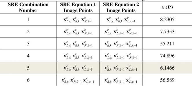
Table 4.2 Four combinations of the scale restraint equation in four views ... 83

Table 4.3 Dimension of the parameter vector (COL vs. SRE) ... 89

Table 4.4 Matrix operations and the corresponding number of flops ... 90

Table 4.5 Flops count required for computing COL ... 92

Table 4.6 Flops count required for computing SRE ... 93

Table 4.7 SRE stereo auto-calibration parameter ... 97

Table 4.8 Square-root of the trace of the parameter variance-covariance ... 98

Table 4.9 Left camera lens distortion parameters ... 101

Table 4.10 Right camera lens distortion parameters ... 101

Table 4.11 Relative orientation of right camera w.r.t left camera (†Free parameter) ... 102

Table 4.12 Number of points and parameters ... 102

Table 4.13 Image distortion coefficients combinations ... 104

Table 4.14 The correlation coefficients of the focal length error ... 106

Table 4.15 The correlation coefficients of the principal point error ... 106

Table 4.16 Left camera lens distortion parameters ... 108

Table 4.17 Right camera lens distortion parameters. ... 108

Table 4.18 Baseline and relative orientation estimates. †Free parameter. ... 108

Table 4.19 Number of the points and parameters ... 109

Table 4.20 Means, standard deviations and RMS of the deviations between the corresponding 3D reference points and estimated points. ... 110

Table 4.21 Means, standard deviations and RMS of the image residuals. ... 110

Table 5.1 The dimensions of the state vectors in the KF, KF-ST and KF-PTC ... 135

Table 7.1 Crossbow IMU440CA technical specification (partial) ... 165

Table 7.2 Dataset properties... 166

Table 7.3 IMU440CA sensor error model parameters ... 168

Table 7.4 The lens distortion parameters with the left camera ... 174

Table 7.5 The lens distortion parameters with the right camera ... 175

Table 7.6 The relative orientation of the right camera w.r.t the left camera. ... 175

(11)

xi

Table 7.8 Difference between the estimated and measured lever arm components 176

Table 7.9 Number of points, objects, iterations, flops and ˆ₀2 ... 177

Table 7.10 COL, SRE1 and SRE2 parameter list and size ... 177

Table 7.11 Average number of points per frame used in each section. ... 182

Table 7.12 The VO translation and rotation drift rates ... 184

Table 7.13 The mean, standard deviation and rms of the differences between the VO and GNSS-aided inertial integrated navigation solution ... 190

Table 7.14 The translation and rotation drift rates from the VO-aided inertial integrated navigation ... 194

Table 7.15 The translation and rotation drift rates from the TC SLAM and TC MFVO algorithms ... 202

(12)

xii

List of figures

Figure 2.1 Overview of a typical IA-INS system ... 18

Figure 2.2 Matching of point features from a pair of stereo frames ... 19

Figure 3.1 The i-, e-, n-, nc-, b-, c- and n’- frames. ... 44

Figure 3.2 GNSS Pseudorange positioning ... 45

Figure 3.3 Inertial navigation mechanization [Grewal et al, 2013] ... 55

Figure 3.4 Loosely coupled GNSS/IMU integration architecture ... 57

Figure 3.5 Tightly coupled GNSS/IMU integration architecture ... 57

Figure 3.6 The collinearity condition ... 61

Figure 3.7 Two view geometry ... 62

Figure 3.8 Three view geometry ... 63

Figure 3.9 The geometrical relationship between an IMU and ... 67

Figure 3.10 The corner (left) and blob (right) masks ... 71

Figure 4.1 Stereo Vision ... 80

Figure 4.2 Four view feature matching (left) and ... 82

Figure 4.3 The six possible combinations to constrain four views with two SREs ... 84

Figure 4.4 Two and three overlapping regions. ... 85

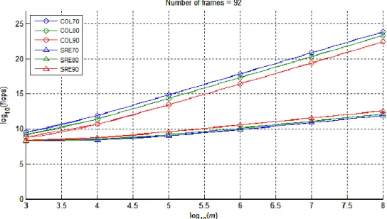
Figure 4.5 Flops vs. number of stereo points (m) ... 94

Figure 4.6 The 2D trajectory, landmarks (left) ... 95

Figure 4.7 3D trajectory, landmarks in view, left image and right image at epoch 46 ... 96

Figure 4.8 Number of stereo points per frame vs. epoch ... 97

Figure 4.9 The number of the stereo points per frame (top) ... 99

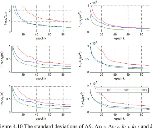
Figure 4.10 The standard deviations of ∆fL, ∆xL,0, ∆yL,0, kL,1, kL,2 and kL,3 ... 99

Figure 4.11 The standard deviations of ∆fL, ∆xL,0, ∆yL,0, kL,1, kL,2 and kL,3 ... 100

Figure 4.12 Stereo Camera System with IMU (Left). 90x60cm Checkerboard (right) ... 103

Figure 4.13 Image measurements for the calibration ... 103

Figure 4.14 X, Y, Z and 3D ranging errors for combinations 1 to 8 ... 105

Figure 5.1 Timeline between epochs k-m and k. ... 115

Figure 5.2 Overlap of frames k-2, k-1 and k. ... 129

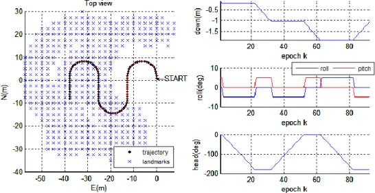
Figure 5.3 The top view of the vehicle trajectory with visible landmarks (left) ... 132

(13)

xiii

Figure 5.5 True position and heading RMSE (left) ... 135

Figure 5.6 Loosely-coupled VO aided-inertial navigation with... 139

Figure 6.1 j as a function of overlap percentage ... 151

Figure 6.2 The top view of the vehicle trajectory with the visible landmarks (left) 152 Figure 6.3 The true position and heading RMS errors (left) ... 154

Figure 6.4 The dimensions of the state vectors with SLAM and MFVO, ... 155

Figure 6.5 The comparison between the VO/KF-PTC and MFVO approaches ... 156

Figure 6.6 Tightly coupled MFVO aided-inertial navigation ... 159

Figure 7.1 GPS and IMU, and Controller in YUMIS system [Qian, 2017] ... 164

Figure 7.2 The 2D overview of the trajectory with starting point, end point and base position (left) and the velocity and attitude profiles (right) ... 166

Figure 7.3 The GPS position standard deviation (1-σ) (top-left). ... 167

Figure 7.4 The estimated position accuracy (1-σ) and orientation accuracy (1-σ) .. 169

Figure 7.5 The GPS system innovations (left) ... 169

Figure 7.6 The estimated accelerometer and gyroscope biases... 170

Figure 7.7 The calibration interval (left) and a stereo pair with the matched points (right) ... 171

Figure 7.8 The number of the features (top), the minimum, mean and maximum ranges of the 3D features (bottom) for COL, SRE1 and SRE2. ... 173

Figure 7.9 The sstandard deviations of the EO parameter for the image frames ... 173

Figure 7.10 The thirty-five 200m sections with Section ID ... 179

Figure 7.11 The numbers, and mean ranges of the 3D features for the divided sections. The colors of the plot corresponds the sections in Figure 7.10. ... 180

Figure 7.12 3D position and orientation drifts of the individual sections ... 183

Figure 7.13 The visual odometry solution; the position change (top) ... 188

Figure 7.14 The standard deviation (1-σ) of the VO solution ... 188

Figure 7.15 The number of the features at each epoch (top), the minimum, average and maximum object feature ranges (middle), and the percentage of the shared features between the current and previous VO solution epochs (bottom). ... 189

Figure 7.16 The differences between the VO and GNSS-aided... 190

Figure 7.17 The 2D overview of Section 27 (best) and Section 25 (worst) ... 192

Figure 7.18 The drifts in 3D position and orientation from KF, KF-ST and KF-PT for the individual color coded sections ... 193

Figure 7.19 Section 27 position change system innovation and 1-σ error bounds... 195 Figure 7.20 Section 27 orientation change system innovation and 1-σ error bounds 196

(14)

xiv

Figure 7.21 The system innovations of the position changes and 1-σ error bounds .. 196 Figure 7.22 The system innovations of the orientation changes and 1-σ error bounds

... 197 Figure 7.23 The drifts in 3D position and orientation from ... 200 Figure 7.24 The size of the state vector (top). The number of features per frame and

the average number of features per frame during the respective sections (middle). ... 203 Figure 7.25 The histograms of the standardized system innovation vectors... 204

(15)

xv

List of symbols

By convention vectors are represented by boldface lowercase characters and matrices by boldface uppercase characters.

 pitch angle

y x

θ vector of Euler angles from x-frame to y-frame

 geodetic longitude

 roll angle

φ rotation vector or rotation vector error of a DCM

 geodetic latitude

 heading or yaw angle

ψ rotation vector error of a DCM

e



magnitude of the rotation rate of the Earth (7.2921158×10-5 rad s-1)

z xy

ω angular rate vector of the y-frame with respect to the x-frame projected to the z-frame

z xy

Ω skew symmetric matrix of vectorωz_xy

Φ transition matrix

 standard deviation

2 0

 variance factor

 coefficient matrix of the process noise

0 zero vector

(16)

xvi

y

a acceleration vector in the y-frame

b baseline vector

a

b accelerometer bias vector g

b gyroscope bias vector

i

C DCM rotation matrix about the i-axis y

x

C 3D transformation matrix from x-frame to y-frame d system innovation vector

e first eccentricity of a reference ellipsoid

f focal length (.) (.),f f system function h ellipsoidal height ) ( h ,h() measurement function x H

H, Jacobian matrix a model at the parameter/states vector

z

H Jacobian matrix a model at the measurement vector

I identity matrix

K Kalman gain matrix

y

la

lever-arm vector in the y-frame y

l position vector of 3D features in the y-frame N matrix of normal equations

y

m SLAM landmark position vector in the y-frame

(17)

xvii

Q covariance matrix of the process noise vector

r geographic position vector (latitude, longitude, height) R covariance matrix of the measurement vector

E

R curvature radius of meridian

N

R curvature radius of prime vertical

s

,

s scale factor, scale factor vector

S covariance matrix of the system innovation vector

k

t time t at epoch k

wprocess noise vector

W weight matrix

x state vector or parameter vector z

y

x, , Cartesian coordinates in the image space in the y-frame y

x position vector in the image space in the y-frame Z

Y

X, , Cartesian coordinates in the object space in the y-frame y

X position vector in the object space in the y-frame

v measurement noise vector

y

v velocity vector in the y-frame

(18)

xviii

List of operators

i

 the ith element of a vector

ij

 ,i,j the i th

row and the jth column element of a matrix

k

 epoch k (as the subscript)

x

 x- component of a 3D vector (as the subscript)

y

 y- component of a 3D vector (as the subscript)

z

 z- component of a 3D vector (as the subscript) ) (t  a function of time   perturbation of 

ˆ an estimated or adjusted value



a computed value

) 0 (

 an approximate value (as the superscript) 

 a time update (prediction) in a Kalman filter (as the superscript) 

 a measurement update in Kalman filter (as the superscript)  the dot product operator

 the cross-product operator or multiplication operator



 the skew-symmetric form of a vector T

 transpose of a vector or a matrix T



 transpose of a matrix inverse or vice versa



 difference, change



(19)

xix . the absolute value

. the Euclidean norm



Boolean equal operator

 is approximately equal to ]

,

[a b the interval between a and b

) (

c the cosine operator

) (

ceil the ceiling function )

(

chol the lower triangle Cholesky operator )

(

diag the diagonal matrix in the form of a vector or block matrices ]

[

E the expectation of a variable or a vector (.)

exp an exponential function )

(

s the sine operator

) (

sqrt the square root operator )

(

(20)

xx

List of abbreviations and acronyms

2-D two dimensional 3-D three dimensional a.k.a. also known as

BA bundle adjustment

CCD charge-coupled device

CMOS complementary metal–oxide–semiconductor COL collinearity equations

DCM direction cosine matrix ECEF Earth-Centered Earth Fixed EKF extended Kalman filter EO exterior orientation d.o.f. degrees of freedom

GM Gauss-Markov

GMST Greenwich Mean Sidereal Time GNSS Global Navigation Satellite System IBN image-based navigation

IMU inertial measurement unit INS inertial navigation system IO interior orientation

KF Kalman filter

LiDAR light detection and ranging

(21)

xxi n/a not available

max maximum

MEMS Micro-Electro-Mechanical Systems MFVO multi-frame visual odometry

min minimum

px pixels

RANSAC random sample consensus rms root mean square

RTK real-time kinematic

SLAM simultaneous localization and mapping SRE scale-restraint equation

VCV variance covariance

WGS84 World Geodetic System 1984 w.r.t. with respect to

(22)

1

1. Introduction

This chapter provides an introduction to this dissertation. Section 1.1 contains a background which is followed by the research objectives in Section 1.2. And finally Section 1.3 outlines the dissertation.

Background

1.1.

The high demand for direct-georeferencing technology with low-cost multisensor integrated kinematic positioning and navigation systems in mobile mapping and direct georeferencing is continuously driving more research and development activities. Mobile mapping involves the collection of data to produce maps while in continuous motion. GNSS aided-inertial navigation systems are widely used for making maps efficiently on mobile platforms through direct georeferencing, The direct georeferencing method uses the position and orientation information to geo-code each pixel or point collected by a camera or LiDAR system, respectively, without the use of extensive ground control points. The position accuracy of the georeferenced pixels or points depends on the accuracy of navigation solution.

GNSS provides long term high accuracy of absolute position and velocity solution but does not work in indoor or urban-canyon environments. INS, on the other hand, works in all environments but its solution accuracy deteriorates with time. An integrated GNSS-INS system can take their advantages to determine the trajectory of a moving platform in position, velocity and attitude and so on. During any GNSS outage the accuracy of the navigation solution depends solely on the quality of inertial navigation sensors. Navigation and tactical grade of inertial measurement units (IMUs) exhibit low solution

(23)

2

drift rate but are very expensive and not easily accessible to the public in civilian applications. Hence, more and more low-cost IMUs have been made available during the past decade. Low grade of MEMS IMUs are considerably cheaper and easily available but accumulate large errors over a relatively short period of time. To reduce the INS errors in poor GNSS or GNSS denied environments, other sensors can be added to the navigation system, for example Wi-Fi positioning, barometer, odometer and magnetometer to name a few [Aggarwal et al, 2010]. In the past decade, image-aiding has become a hot topic in multisensor integrated navigation. Cameras are inherently high-bandwidth and therefore have the high potential for very precise angular resolution and are readily available and easy to interface with [Miller et al, 2011]. Furthermore, it is inexpensive in comparison with other self-contained electro-optical sensors such as laser ranging (LIDAR) [Shen and Liu, 2005].

In order to use cameras as navigation sensors, they have to be calibrated first, which refers to the determination of the focal length, the principal point offset and the image distortion parameters. Furthermore, the determination of the translational offsets and the orientation (boresight) angles between the individual sensors in a multi-sensor system are also part of the calibration. Usually, the traditional camera calibration consists of capturing images containing an array of the reference targets with their coordinates accurately known in a laboratory [Wolf and Dewitt, 2000]. However, such methods require the setup of enough reference points and the calibrated parameters can become invalid during field operations, e.g., due to camera assembly/disassembly, replacement and/or bumps [Teller et al, 2010].

(24)

3

Alternative to the traditional calibration techniques are the auto-calibration (or self-calibration) methods. An auto-calibration refers to the determination of the camera parameters from a sequence of the overlapped images without setting up ground control points (GCPs) or specific calibration targets. The main advantages are: (a) the procedure can be fully automated, (b) the calibration can be performed in-field, and (c) the accuracy of the estimated calibration parameters can be improved by the applied information from other sensors in the system. Typically, an auto-calibration is performed in a bundle adjustment based on the extended collinearity equations where the interior orientation parameters (IOPs), the exterior orientation parameters (EOPs) and the object coordinates (a.k.a. landmark coordinates) are estimated. However, they are computationally expensive due to the very large number of object position parameters.

Another way of performing the auto-calibration is through structureless bundle adjustment methods [Faig, 1975; Cefalu et al, 2016]. These methods are based on the epipolar and scale consistency constraints and are free from object coordinates. The number of unknown parameters in the bundle adjustment is drastically reduced. Hence, this PhD research developed a camera calibration method that could precisely calibrate camera parameters in a GNSS/IMU/Stereo cameras integrated system exclusive of the object coordinate parameters. It applies the three-view scale-restraint equation [Bethel, 2003; Ghosh, 2005], with which the measurements are processed exclusively in the image space. Therefore, it does not allocate large memory and computing resources.

Once the cameras are calibrated, they are ready for navigation. There are two main analytical approaches to extract navigation information from image measurements, namely visual Simultaneous Localization and Mapping (SLAM) and visual odometry

(25)

4

(VO) [Murcott et al, 2011]. The former simultaneously determines the motion and the map while the latter only focuses on the motion of consecutive frames. The advantage of SLAM is that the navigation accuracy can be increased by detecting and applying loop-closures in scenarios when the same locations are visited more than once [Liu and Zhang, 2012]. However, this benefit does not hold when the same locations are not revisited and absolute positioning information, such as GNSS or position fixes, are available. The main drawback with the SLAM is the increase of the computational requirement as more and more landmarks are added to the map. The VO, on the other hand, can maintain a constant dimensionality in system parameterization since the output is only the pose changes of a moving object and does not take up a large memory.

The fusion of imaging and inertial sensors can be performed using batch processing methods [Indelman et al, 2013b; Leutenegger et al, 2015; Forster et al, 2017] or using a Kalman filter[Veth et al, 2006; Mourikis et al, 2009; Sazdovski et al, 2011; Bloesch et al, 2015; Liu et al, 2016]. The Kalman filter is generally preferred since the data processing is conducted sequentially epoch after epoch. Furthermore, GNSS-aided inertial navigation via a Kalman filter is well-known so that it is natural to employ Kalman filtering for image-aiding in the GNSS/IMU/stereo cameras integrated kinematic positioning and navigation. The SLAM-based image-aiding method [Sazdovski et al, 2011] uses the standard form of the extended Kalman filter and does not require any modification to the current GNSS-aided INS architectures. The VO-based image-aiding methods, however, require special attention to the following two specifics with the pose changes: (a) they are relative in nature and (b) pairwise correlated in terms of time. The relative measurements can be processed using the stochastic cloning Kalman filter

(26)

5

[Roumeliotis et al, 2002], which relates the positions and attitudes of a moving vehicle between two consecutive image frames. A shaping filter, which is a differential or difference equation with white noise input and output of a certain correlation function [Grewal, 2001], is usually used to model time-correlated measurements. The state vector is then augmented with the state vector components of the shaping filter and the resulting system model is in the form of a linear dynamic system driven by white noise [Grewal, 2001]. However, the conventional shaping filter for time-correlated measurements in [Bryson and Henrikson, 1968; Gelb, 1974] does not adequately model the pairwise time-correlated case and is therefore suboptimal with its application in the VO aided inertial navigation.

Similar to any dead-reckoning navigation technique, the incremental VO estimates accumulate errors and drifts over time. The drifts in the VO estimates can be reduced by utilizing image measurements from more than two consecutive frames; specifically, the last m frames (m > 2). This approach has been employed in [Mourikis and Roumeliotis 2007; Fraundorfer et al, 2010; Clement et al, 2015; Wen et al, 2016], where the pose and feature positions are jointly estimated at the local level. However, the number of parameters in these methods increases as more features are observed and could become impractical when the dimension of the parameter vector is too high. Furthermore, the optimal integration of multi-frame image measurements in the current state-of-the-art GNSS aided inertial navigation is not so obvious.

This dissertation is focused on developments of theoretical and practical techniques for image and IMU integration. Two image-IMU integration algorithms were developed: (a) loosely-coupled visual odometry aided inertial navigation (LC VO aided-INS) and (b)

(27)

6

tightly-coupled multi-frame visual odometry aided inertial navigation (TC MFVO aided-INS).

The LC VO aided-INS employs a Kalman filter algorithm that models the pairwise time correlated VO measurements. The shaping filter for this type correlation uses Cholesky factors as the coefficients derived from the variance and covariance matrices of the measurement noise vectors. The state vector is then augmented with the de-correlated measurement noise vector which results in the form of the standard Kalman filter. The test results showed that the proposed algorithm performs better than the existing Kalman filter algorithms and provides more realistic covariance estimates.

The TC MFVO aided-INS algorithm integrates image data from multiple stereo frames without involving feature positions in the state vector. The measurement equation system in this MFVO is derived from the SLAM measurement equation system where the landmark position parameters are algebraically eliminated by time-differencing the measurements at two consecutive epochs. However, the resulting time-differenced measurements are time-correlated. Through a sequential de-correlation algorithm, the Kalman filter measurement update can be performed sequentially and optimally. The proposed MFVO algorithm uses far less computation resources while producing identical navigation solution in comparison with the SLAM method.

The derived system and measurement equations for both the LC VO aided-INS and the TC MFVO aided-INS algorithms are in the form of the standard Kalman filter. Therefore, they can be easily integrated into the current state-of-the-art GNSS aided-INS architectures.

(28)

7

Research objectives

1.2.

The objectives of the dissertation are to:

 Design, implement and evaluate a structureless camera auto-calibration and system calibration for a GNSS/IMU/Stereo camera integrated system based on the scale-restraint equation. Compare (a) the accuracy of the estimated calibration parameters and (b) the computational complexity of the proposed method with the auto-calibration algorithm based on the collinearity equations.

 Develop Kalman filter algorithm for processing pairwise time-correlated measurements. Then, implement the algorithm in a loosely coupled stereo VO aided-INS. Finally, evaluate and compare the accuracy of the proposed algorithm with the standard Kalman filter and the Kalman filter with the conventional time-correlated measurements.

 Develop and implement an optimal technique for fusing the multi-frame visual odometry and IMU measurements. Then, evaluate and compare the performance of proposed method to visual SLAM aided-INS.

Dissertation outline

1.3.

The remainder of the dissertation is structured as follows: Chapter 2 gives a literature review of multisensor fusion and integration navigation, camera calibration and image-aided inertial integrated navigation while Chapter 3 summarizes the fundamentals of estimation theory, GNSS, inertial navigation and image-based navigation. Right after, the structureless camera auto-calibration and system calibration algorithms for a GNSS/IMU/Stereo camera integrated are developed in Chapter 4. Chapter 5 presents the

(29)

8

loosely-coupled visual odometry aided inertial navigation. Then, the tightly-coupled Kalman filter is presented for fusing multi-frame visual odometry and INS tightly coupled stereo multi-frame aided inertial navigation algorithm in Chapter 6. Chapter 7 further gives the test results and conducts performance analysis of the proposed algorithms developed in Chapters 4, 5 and 6 using data collected from YUMIS system by the EOL lab of York University. At the end, Chapter 8 summarizes the dissertation with the conclusions of the research and recommendations for future work.

(30)

9

2. Literature review

This chapter contains a literature review. Section 2.1 focuses on camera calibration while Section 2.2 focuses on reviewing image-aided inertial integrated navigation.

Camera auto-calibration and system calibration

2.1.

Image-based navigation (IBN) algorithms assume that the camera system is geometrically calibrated prior to its use and the calibration parameters do not change over time. There are many definitions of camera calibration in the literature. In general, regardless of the various definitions, a camera is considered as calibrated if its focal length, principal point offset and image distortion parameters are known [Remondino and Fraser, 2006]. The determination process of these parameters is referred to as camera calibration. In photogrammetry, the mathematical model for camera calibration involves the extension of the collinearity equations through additional parameters that model the distortions. The distortion model generally requires five or more point correspondences from multiple overlapping images and is fit through a least-squares bundle adjustment [Remondino and Fraser, 2006].

In multisensor integrated system consisting of a stereo camera system, the translational offsets and the orientation angles between the individual sensors are unknown after assembly. In a GNSS, IMU and stereo cameras integrated system, these geometric parameters are the 3D baseline vector and the relative orientations between two cameras [Prokos et al, 2012], the lever-arms and bore-sight angles [Bender et al, 2013] of the reference camera with respect to a specific reference point of the system. The determination of these unknowns is referred as system calibration.

(31)

10

There are different camera and system calibration techniques that solve some or all the parameters and can be categorized as follows:

Laboratory calibration: determines the focal length and principal point offset using goniometers, compactors, collimators or other optical alignment instruments in a laboratory setting [Clarke and Fryer, 1998, Wolf and Dewitt, 2000, Ghosh, 2005]. This type of the methods is usually employed in high accuracy metric cameras and almost never in low- cost off-the-shelf cameras.

Traditional calibration: consists of capturing images containing an array of the 3D reference targets, whose coordinates are accurately known i.e., pre-surveyed [Wolf and Dewitt, 2000]. The reference targets can be in two or three planes orthogonal to each other [Zhang, 2004] or in a calibration cage [Moe et al, 2010]. These methods provide a very accurate calibration results but are expensive to setup and maintain. An easier setup is to employ planar grid, such as checkerboard [Zhang, 2000]. It is reasonably accurate, simple to produce and more practical to use. The parameters are usually estimated through a bundle adjustment or the Levenberg-Marquardt algorithm [Remondino and Fraser, 2006]. However, these parameters are calibrated in such an environment that may not necessarily be the same as the real working environment.

Auto (or self) -calibration: performs the calibration by using a sequence of the overlapping images without the use of any reference target and does not require an elaborate setup. The calibration can be performed in any environment with texture and close-range objects. The methods in this category are therefore more flexible and practical than the traditional methods. However, they may not be able to achieve the same accuracy level as traditional methods. Besides, the absolute scale of the camera

(32)

11

system cannot be known without additional information. Similar to the Traditional calibration methods, the calibration parameters are estimated through a bundle adjustment (BA) or the Levenberg-Marquardt algorithm.

System calibration: involves the determination of lever-arms [Bender et al, 2013], boresight angles [Mostafa, 2001] and the absolute scale of the camera system [Kelly el al, 2011] in a multisensor integrated system. These parameters can only be obtained via external information. For example, lever-arms can be measured using survey equipment, boresight angles can be recovered with GCPs and the absolute scale can be estimated using GNSS measurements as the reference.

In-field (or in-flight) calibration: can be considered as a combination of the traditional, auto and system calibration methods. This is performed when system calibration parameters are not available or become invalidated during in-field operations, e.g., due to camera assembly/disassembly, replacement, or bumps [Teller et al, 2010].

2.1.1. Auto-calibration

The most widely used mathematical model for camera auto-calibration is the well-known extended collinearity, which consists of the collinearity equations and the image distortion model [Fraser, 2012]. The auto-calibration procedure can be categorized into block-invariant [Kenefick et al, 1972; Ghosh, 1988] and photo-variant [Moniwa, 1980] approaches. The former assumes that the distortion is constant in a set of images, while the latter assumes that the distortion changes between images. Most auto-calibration approaches involving digital cameras are block-invariant.

The calibration parameters can be determined in a bundle adjustment (BA) [Ghosh, 1988; Triggs et al, 2000] or in the SLAM framework [Civera et al, 2009; Kelly and

(33)

12

Sukhatme, 2009; Kelly et al, 2011; Keivan and Sibley, 2014]. This process involves the simultaneous estimation of the calibration parameters, the exterior orientation and the positions of the stationary objects. In photogrammetry, BA is the preferred method for this purpose. The parameters are usually estimated by using least-squares (LS) [Triggs et al, 2000] or the Levenberg-Marquardt (LM) algorithm [Levenberg, 1944; Hartley and Zisserrnan, 2003]. The size of the computed Jacobian matrix and normal equation system can be large. Solving this linearized system can be inefficient in terms of the memory and computation loading and can be impractical especially when the number of the involved exterior orientation parameters and the involved objects is large [Jeong et al, 2012].

There are several methods proposed to reduce the computation and memory load in the BA by exploiting the sparsity of the Jabobian matrix and normal equation. Lourakis and Argyros [2009] presented the Sparse Bundle Adjustment (SBA) by constructing a dense normal matrix from the non-zero Jacobian blocks, in which the Cholesky decomposition and back-substitution method were used to solve the parameters. Konolige [2010] improved the efficiency of the SBA with the Sparse Sparse Bundle Adjustment (sSBA) by employing a highly-optimized Cholesky decomposition solver. The efficient Incremental Smoothing and Mapping (iSAM) algorithm was developed by Kaess et al [2008], where the parameters were updated by a QR factorization of the naturally sparse normal matrix and by only re-computing matrix entries that actually changed. Kaess et al [2011] further improved variable reordering and re-linearization in iSAM2 by implementing a Bayes tree data structure. Although these have methods have improved the computationally efficiency of solving the BA problem, the number of estimated parameters can still be large. As an example, consider a set 100 stereo images viewing

(34)

13

10000 objects. The total number of parameters the being estimated in the BA is 30625 (see Table 2.1) and 98% of them are the position vector of the objects. The object coordinates are not particularly in need since the goal is to obtain the calibration parameters. If they can be removed or omitted from the system of equations, then the memory and computational usage for solving the BA problem can be drastically reduced.

Table 2.1 The components of the parameter vector and the corresponding size in a stereo camera auto-calibration bundle adjustment

Number of stereo images 100

Number of observed objects 10000

Parameter Size

Focal length error, principal point error 2×3 Image distortion (10 parameter model) 2×10 Stereo baseline and relative orientation (one

baseline component is fixed) 2+3

Exterior Orientation (one EO parameter is fixed) 6×(100-1)

Object position parameters 3×10000

Total parameter vector size 30625

Several approaches have been proposed to reduce the order of the BA. Dang et al [2009] introduced a BA with the reduced order for their stereo self-calibration algorithm. The x and y components of the object positions were algebraically eliminated from the equation system, only the depth (z) component of the objects remains in the parameter vector, which reduced the parameter dimension by almost 2/3. The Schur complement trick was used in [Triggs et al., 2000, Jeong et al, 2012] where the dimension of the linear equation system was reduced such that only exterior orientation (EO) parameters were estimated. These methods are useful for cases where only the EO parameters are required by the user. However, the Jabobian matrix requires a good approximation of the object positions which can be difficult to obtain if the camera system is not calibrated.

(35)

14

Calibration methods that are free of object coordinates are referred as structureless BA or light BA. They typically employ two-view constraints, e.g. the coplanarity equations, or three view constraints, e.g. the trifocal tensor [Hartley, 1997], or both. Faig [1975] developed an auto-calibration method which employed the coplanarity equation. Furthermore, a control restraint condition was included to recover the absolute orientation of the images. More recently, Rodriguez et al. [2011a, 2011b] developed the Global Epipolar Adjustment (GEA) using the two-view coplanarity constraint in their bundle adjustment. Cefalu et al [2016] implemented a similar approach as in [Rodriguez et al., 2011b], which included the image distortion model into the measurement equation by Brown [1971]. It has shown that the GEA required less number of iterations than the SBA using the LM algorithm. Furthermore, the number of parameters is fixed per image pair. However, the estimated translation vectors between the images are ambiguous and do not have physical meaning since coplanarity constraint does not ensure that all images are with the same scale. Scale consistency is important in a multisensor integrated navigation system and for general applications. Three view constraints can be used to ensure the scale consistency between the views. Steffen et al. [2012] proposed a structureless relative BA which combined the epipolar and trifocal constraints between images. The relative representation of the camera positions improved the numerical condition of the equation system and is also statistically equivalent to the classical bundle adjustment. Indelman [2012] implemented the incremental light bundle adjustment (iLBA) and derived a three-view constraint system involving three equations, i.e., two epipolar equations and a third three-view constraint equation, for the scale consistency. Indelman et al. [2013a] integrated the iLBA with IMU measurements for robotic

(36)

15

navigation. Both Steffen et al. [2012] and Indelman [2012] used monocular vision and chained the entire image set by constraining images {1, 2, 3}, then images {2, 3, 4}, and so forth. This chaining ensures that all images operate on the same scale. However, they assumed that the cameras have been calibrated.

Auto-calibration algorithms have a rank deficiency of order seven (i.e. 3D position, 3D orientation and scale). Hence, they require the minimal constraints to define the network datum, which can be done by applying the minimum constraint free-network adjustment, or through explicit minimal control point [Remondino and Fraser, 2006]. In free-network adjustment one can fix one camera position and one orientation. Then one coordinate component of a second position or the distance between the two cameras can be fixed [Cefalu et al, 2016]. If stereo cameras are used, then the length of the stereo baseline is treated as a free parameter [Hartley and Zisserman, 2003]. In order to recover the absolute scale, certain external information is needed.

2.1.2. System calibration

The boresight angles between an IMU and a camera system can be determined with or without ground control points (GCPs). In the first case, the camera orientation is first computed using GCPs. Then the IMU body-to-mapping frame direction cosine matrix (DCM) is determined at the time of exposure. Finally, the boresight angles are recovered by comparing the two sets of orientations [Škaloud et al, 1996, Mostafa, 2001]. In the second case, the boresight angles are treated as constant parameters in a bundle adjustment [Pinto, 2002, Heipke et al, 2002, Mostafa, 2002, Bender et al, 2013]. These two methods are typically applied in calibrating aerial photogrammetric survey systems with the known IO parameters.

(37)

16

Camera-IMU lever-arms can be measured using survey equipment or estimated in the BA. Bender et al [2013] presented an in-flight graph based the BA approach for system calibration between a rigidly mounted camera and an IMU. Image point features together with the solution of the GNSS aided-inertial navigation position and orientation were used as measurements. This method simultaneously computed the IOPs as well as the lever arms and boresight angles between the two systems. However, it also required one GCP at least in-order to recover the z-component of the lever-arm vector. Kelly and Sukhatme [2009] proposed a camera-IMU self-calibration method within the SLAM framework implemented by an unscented Kalman filter. The lever-arms and mounting angles, the IMU gyroscope and accelerometer biases, the local gravity vector and landmarks could all be recovered from camera and IMU measurements alone. However, they assumed that the internal camera parameters were known beforehand. Mirzaei and Roumeliotis [2008] presented a similar tightly-coupled approach using an iterative extended Kalman filter, but, in need of known landmark position.

Auto-calibration algorithms in free-network adjustment mode require external information to compute absolute scale of the camera system. Kelly el al [2011] focused on determining the absolute scale of both the scene and the baseline in a stereo rig using GNSS measurements. Their approach was similar to the photogrammetric BA and the structure from motion algorithms. They could recover the baseline and the relative orientation between the two cameras and the lever-arms between the GNSS antenna and the reference camera.

Accordingly, this dissertation develops a camera auto-calibration algorithm using a structureless bundle adjustment for a stereo camera system. Furthermore, system

(38)

17

calibration is performed using GNSS/IMU data to recover the boresight angles, lever-arms and absolute scale of the camera system. Both camera auto-calibration and system calibration parameters are estimated simultaneously using the least square method.

Image aided-INS integration

2.2.

In an image aided-INS (IA-INS), the performance of the inertial navigation system can be improved by fusing the measurements derived from images taken by an on-board camera system. Typically, point features are extracted and matched from consecutive overlapping image frames using image processing techniques. Then the IA-INS algorithm uses these point features as measurements to estimate the navigation states via batch processing [Indelman et al, 2013b; Leutenegger et al, 2015; Forster et al, 2017] or a Kalman filter[Veth et al, 2006; Mourikis et al, 2009; Sazdovski et al, 2011; Bloesch et al, 2015; Liu et al, 2016].

The camera system can consist of a single or stereo camera. Monocular vision can only estimate the trajectory only up to an unknown scale. Stereo vision, on the other hand, avoids the scale ambiquity inherent in monocular vision when the stereo baseline is known. Furthermore, monocular vision requires three consecutive frames in order to transfer the relative scale and this tends to reduce the stability of the system [Scaramuzza and Fraundorfer, 2011].

Since the early 1980s, IA-INS research has been conducted. Moravec [1980] introduced one of the first image-only motion estimation using stereo cameras. Merhav and Bresler [1986] developed an online image-based velocity-to-height ratio estimation algorithm and its integration with on board navigation sensors. With the availability of digital cameras in the 1990s, the typical data process of modern IA-INS consists of three

(39)

18

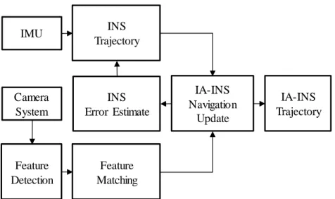
main steps (a) point feature detection (b) point feature matching and (c) pose (or pose change) estimation and navigation state update. Figure 2.1 overviews a typical modern IA-INS.

Figure 2.1 Overview of a typical IA-INS system

In the feature-detection step, stable points, such as corners and blobs, are located on the images. For navigation applications, the detector must be repeatable, i.e. it should ideally be able to find the same point features in multiple frames. Many feature detectors have been developed, for example, Harris [Harris et al., 1988], SIFT [Lowe, 1999] and SURF [Bay et al., 2008]. Once the features have been identified in each frame, they are matched across multiple frames. This is achieved by first constructing a feature descriptor using pixels around the point. The descriptor vectors on an image are then matched against descriptors from other images in order to obtain correspondences. Constrained matching techniques can be employed to reduce the number of potential matching candidates and there can reduce the search time. In the case of stereo vision, the search can be performed along the epipolar lines between the stereo pairs [Bin Rais, et al, 2003]. Between consecutive frames, the locations of the features on the next frame can be

Camera System INS Trajectory Feature Matching IA-INS Navigation Update IMU IA-INS Trajectory INS Error Estimate Feature Detection

(40)

19

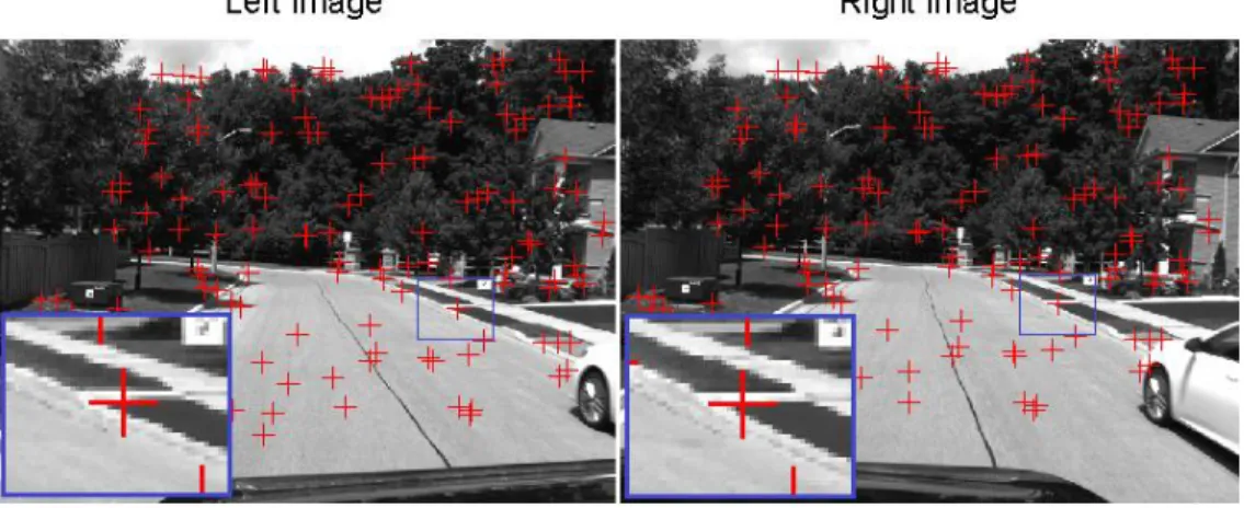
predicted using a motion model [Scaramuzza and Fraundorfer, 2011] or using the motion estimate from the inertial navigation solution [Veth et al, 2006]. This can effectively reduce the search radius, increase the efficiency and help to prevent aliasing. Figure 2.2 shows point features extracted and matched from a stereo pair.

Figure 2.2 Matching of point features from a pair of stereo frames

The pose estimation and navigation state update are typically based on visual SLAM [Davison, 2003; Konolige, K and Agrawal, 2008; Alcantarilla et al, 2012] or visual odometry (VO) [Nister et al, 2004; Konolige, et al 2007; Gopaul et al, 2017]. The former applies the well-established SLAM algorithms, while the latter tracks common features from the consecutive image frames [Murcott et al, 2011].

The SLAM technique incrementally builds a consistent map of landmarks in an unknown environment whilst the simultaneous determination of the location of the mobile system is being conducted [Dissanayake et al, 2006; Durrant-Whyte and T. Bailey, 2006a; Thrun et al. 2008]. The state vector consists of the navigation states (position, velocity and/or orientation) and the landmark positions. The SLAM algorithm requires map maintenance where newly visible landmarks observed from the

(41)

20

environment are added to the map and landmarks that are no longer visible or to be revisited are removed from the map.

Visual SLAM tends to be more accurate than VO, since the map retains the memory of the measurements over multiple frames while VO only employs measurements from two latest consecutive image frames [Scaramuzza and Fraundorfer, 2011]. Furthermore, the accuracy of visual SLAM can be increased by detecting and applying any loop-closure in scenarios when any location is visited more than once [Liu and Zhang, 2012]. However, the application of loop-closures may be irrelevant in cases where past locations are not revisited and when absolute position measurements, such as GNSS position or position fixes, become available. Furthermore, the main drawback with the SLAM is the computational load increases in the order of O(n2) , wherein n is the number of landmarks in the map.

The computation complexity can be reduced though approximate and suboptimal methods. Guivant and Nebot [2001] introduced a suboptimal EKF-SLAM method where only a subset of the landmarks’ variance-covariance (VCV) matrix is considered during the measurement update. The VCV estimate then becomes more conservative. Julier [2001] used the Schmidt-Kalman filter, in which only the camera pose and a limited subset of the landmarks are updated. The computational costs become linear in relation to the number of the landmarks in the state vector. Even though suboptimal methods trade optimality for computation and memory usage, they can also degrade or even cause the KF estimates to diverge. Since VO concerns only in determining the trajectory and does not have to deal with landmark positions, it is computationally more efficient than visual SLAM and can work in constant state vector size [Williams and Reid, 2010].

(42)

21

The image-aided inertial integrated navigation can be achieved using a batch processing (e.g. bundle adjustment [Indelman et al, 2013b] and non-linear least-squares [Leutenegger et al, 2015] and graph-based optimization [Forster et al, 2017]) or a Kalman filter [Veth et al, 2006; Mourikis et al, 2009; Sazdovski et al, 2011; Bloesch et al, 2015; Liu et al, 2016]. Batch processing methods process all measurements simultaneously to compute all the parameters. However, these methods can be impractical when the dimension of the parameter vector becomes large. The Kalman filter, on the other hand, is a recursive process, more computationally efficient and more practical. Furthermore, it is preferred since the state-of-the-art GNSS-aided inertial integrated navigation typically employs a Kalman filter.

Similar to multisensor integrated navigation systems in general, the integration schemes of vision-aided inertial navigation can be divided into loosely- and tightly-coupled approaches [Corke el al, 2007]. A loosely-tightly-coupled system consists of two parallel estimation processes that run at different rates and exchange information. The first filter processes the image measurements to obtain the pose or pose change. Then a second filter performs the visual-inertial integration using the output of the first one as measurements. The tightly-coupled approach directly combines image measurements (2D or 3D) and inertial measurements in a single and optimal filter. A loosely-coupled system integrates two well-known subsystems and tends to be computationally more efficient [Leutenegger et al, 2015]. However, the estimation of the camera biases is almost impossible [Li and Mourikis, 2013]. The state vector in tightly coupled systems can include camera biases. However, this requires extensive filter model tuning and increases the computational loading [Corke el al, 2007].

(43)

22

In a VO aided INS [Roumeliotis et al, 2002; Tardif et al, 2010, Sırtkaya et al, 2013], the VO measurement are relative in nature, that is, they are the differences of the positions and attitudes of a moving vehicle between two image frames, from which the VO estimates were derived [Roumeliotis et al, 2002]. The measurement equation is a function of the state vector at the current epoch k and the previous epoch k1 (or some epoch in the past). Equation (2.1) illustrates this model:

k k

k

k h x x v

z  ( , _₁) (2.1)

where z_k is the measurement vector, x_k and x_k_₁ are the state vectors, v_k is the measurement noise vector, and (.)h is the nonlinear measurement model. The current systems augment the state equations to accommodate the relative measurements [Roumeliotis et al, 2002, Konolige et al, 2007, Tardif et al, 2010]. The augmented state vector contains two copies of the original one. The first copy x_k evolves with time, while the second copy x_k_₁ remains stationary. They are then related to each other through the measurement model in (2.1). This approach increases the accuracy of the estimated states and improves the robustness of the system [Roumeliotis et al, 2002].

Another issue with VO is that two consecutive VO estimates are time correlated. The position and attitude change at epoch k is derived from the tracked features at epochs k

and k1. Some of the common features at epoch k1 are also used to derive the relative position and attitude change between epochs k1 and k2. Since there are no common feature points are shared at epochs k and k2, only two consecutive VO measurements (i.e. at epochs kand k1) are correlated. Hence, they are pairwise time-correlated, which was first coined by Bierman [2006]. The Kalman filter in the standard form

(44)

23

assumes that the process noise vector and the measurement noise vector are white and conform to normal distributions with their expectations of zero. However, this assumption is not satisfied with the VO measurements. If the aiding is performed with the standard Kalman filter and the measurement noise vector is colored or time-correlated, the solution of the states will become suboptimal. Neglecting significant time-correlated errors can degrade the performance of the filter. In this case, the Kalman filter is usually augmented with a shaping filter that handles the time-correlated measurements [Bryson and Henrikson, 1968; Gelb, 1974]. However, the commonly used shaping filter as in [Bryson and Henrikson, 1968; Gelb, 1974] not only assumes that the measurement noise are correlated with the ones from the previous epoch, but also with the ones before them, i.e., from epochs k2, k3 and so on. Hence, it cannot appropriately model the pairwise time-correlated measurements. If it is employed in VO-aided inertial integrated navigation, the Kalman filter solution will not produce optimal results. Bierman [2006] introduced a sequential method for whitening pairwise time-correlated measurements for a time series, which uses the Cholesky factors derived from the measurement variances and covariances. The algorithm is efficient, since it is recursive and does not require all the measurements simultaneously available for computation. Mourikis et al [2007] developed the Stochastic Cloning-Kalman filtering equations to deal with pairwise correlated measurements, which involved augmenting the state vector with the feature observations and then estimated camera pose in the following epoch. Although the position and orientation estimates were optimal, the size of the state vector and variance-covariance matrix increases as more observations are made available. This obviously requires more computation and memory resources.

(45)

24

This dissertation proposes a novel method for processing pairwise time-correlated measurements in a Kalman filter. The corresponding shaping filter uses Cholesky factors as coefficients that are derived from the measurement noise variance and covariance matrices. The state vector is augmented with the de-correlated measurement noise vector which results in the form of the standard Kalman filter. The advantages of the proposed algorithm can be summarized as follows: (a) the shaping filter models the VO measurement noise characteristics correctly (b) the Kalman filter can provide a more realistic covariance estimates (c) the size of the state vector is constant and (d) can be easily integrated into an existing GNSS aided-INS architecture.

The drift of VO pose estimates can be reduced by utilizing image measurements from more than two consecutive frames, specifically, the last m frames (m > 2). These approaches, which are often referred as sliding window filter or windowed bundle adjustment, employ batch processing estimators and jointly estimates the vehicle’s pose and feature positions at the local level [Fraundorfer et al, 2010; Clement et al, 2015; Wen et al, 2016]. They have also been implemented in integrated visual-INS systems [Leutenegger et al, 2015; Qin et al, 2017]. Leutenegger et al [2015] employed a non-linear least-squares estimator where the cost function combined the weighted reprojection errors for visual landmarks and inertial error terms for a stereo system. Qin et al [2017] proposed a non-linear optimization-based estimator for a monocular-IMU system using pre-integrated IMU factors. Moreover, they included a procedure for relocalization and loop closure. The number of parameters in these sliding window methods increases as more features are observed and can become impractical when the dimension of the parameter vector becomes too high. Furthermore, it is difficult to integrate these methods