A Software Framework for PCA-based Face Recognition

(1)

A Software Framework for PCA-based

Face Recognition

by

Peng Peng

A thesis

presented to the University of Waterloo in fulfillment of the

thesis requirement for the degree of Master of Mathematics

in Computer Science

Waterloo, Ontario, Canada, 2016

(2)

ii

AUTHOR'S DECLARATION

I hereby declare that I am the sole author of this thesis. This is a true copy of the thesis, including any required final revisions, as accepted by my examiners.

(3)

iii

Abstract

Face recognition, as one of the major biometrics identification methods, has been applied in different fields involving economics, military, e-commerce, and security. Its touchless identification process and non-compulsory rule to users are irreplacable by other approaches, such as iris recognition or fingerprint recognition. Among all face recognition techniques, principal component anaylsis (PCA) was proposed in the earliest stage; however, it is still attracting researchers in this field because of its property of reducing data dimensionality without losing important information.

PCA-based face recognition has been studied for decades. There exist some image processing toolkits like OpenCV, which have implemented the PCA algorithm and associated methods. Nevertheless, establishing a PCA-based face recognition system is still time-consuming, since there are different problems that need to be considered in practical applications, such as illumination, facial expression, or shooting angle, which can hardly be solved by the toolkits. Furthermore, it still costs a lot of effort for software developers to integrate the implementations of the toolkits with their own applications.

Therefore, the thesis provides a software framework for PCA-based face recognition aimed at assisting software developers to customize their applications efficiently. The framework describes the complete process of PCA-based face recognition, and in each step, multiple variations are offered for different requirements. Through various combination of these variations, at least 108 variations can be produced by the framework. Moreover, some of the variations in the same step can work collaboratively and some steps can be omitted in specific situations; thus, the total number of variations exceeds 150. The implementation of all approaches presented in the framework is provided.

(4)

iv

Acknowledgements

I would like to thank Professor Paulo Alencar, for his kindness, understanding and guidance. It has been my honor to be his student and I learned a lot while working with him. I’m very grateful to Professor Daniel Berry for serving as my co-supervisor. Thanks to Professor Donald Cowan for helping me revise my paper and thesis. I also thank Professor Donald Cowan and Professor Ladan Tahvildari for agreeing to read my thesis and providing me valuable feedback.

Immense gratitude towards my parents Zhenyun and Hongwei for their unconditional love. Special thanks to my girlfriend Amy for her constant care and love.

(5)

v

Dedication

(6)

vi

4.1.1 Description ... 39 4.1.2 System Overview... 40 4.1.3 Image Representation ... 41 4.1.4 Face Detection ... 42 4.1.5 Pre-processing ... 45 4.1.6 PCA ... 48 4.1.7 Verification ... 49 4.2 Case study 2 ... 50 4.2.1 Description ... 50 4.2.2 Face Representation ... 52 4.2.3 Face Detection ... 59 4.2.4 PCA ... 61 4.2.5 Verification ... 66

4.3 Other Case Studies ... 67

4.3.1 Case Study 3 ... 67

4.3.2 Case Study 4 ... 70

4.4 Conclusion ... 72

Chapter 5 Conclusions and Future Work ... 73

5.1 Conclusion ... 73

(8)

viii

References ... 76 Appendix ... 80

(9)

ix

List of Figures

Figure 1 Face recognition system ... 7

Figure 2 Learning and classification process ... 9

Figure 3 PCA-based face recognition system flow ... 15

Figure 4 Feature detection [5] ... 17

Figure 5 Eigenfaces [11] ... 18

Figure 6 Original images and projected images [11] ... 18

Figure 7 Framework design model ... 21

Figure 8 Image representation ... 22

Figure 9 Control points [8] ... 25

Figure 10 Shape [8] ... 25

Figure 11 Texture [8] ... 26

Figure 12 Face detection ... 26

Figure 13 Artificial neural network-based method [10] ... 28

Figure 14 Pre-processing ... 29

Figure 15 Face separation [11]... 29

Figure 16 LBP ... 30 Figure 17 LBP weight ... 30 Figure 18 LBP result [11] ... 31 Figure 19 Circle LBP ... 31 Figure 20 LTP ... 31 Figure 21 PCA ... 32

Figure 22 Original dataset [39] ... 33

Figure 23 Eigenvalues and eigenvectors [39] ... 33

Figure 24 Classification by using standard PCA [39] ... 34

Figure 25 Data type [39] ... 34

Figure 26 Original data [39] ... 35

Figure 27 Standard PCA result [39] ... 35

Figure 28 Original data [39] ... 36

Figure 29 Kernel PCA result [39] ... 36

Figure 30 Verification ... 37

Figure 31 Face recognition for smart phones ... 41

Figure 32 Case study 2 ... 51

Figure 33 Case study 3 ... 69

(10)

1

Chapter 1 Introduction

Face recognition has been studied for decades and has been applied in various areas. In 2012, Samsung released their new smart TV which incorporates face recognition by using built-in camera. This new feature allows users to log in to social network applications, such as Facebook, Twitter, or Skype without resorting to a userid and password. In addition, face recognition has also attracted the attention of

governments because of its high security level and accessibility. DARPA (Defense Advanced Research Projects Agency) intends to supplant traditional digital passwords by scanning human faces [1]. Face recognition techniques even can support law enforcement. Karl Ricanek Jr. introduced an application of face recognition in detecting potential child pornography in computer storage. The results show

significant progress in both detection speed and accuracy [2].

Recognizing human faces with computers originates from research in 1964, by Helen Chan and Charles Bisson [3]. Initially, most research focused on detecting individual features, such as eyes, nose, and mouth. As mathematical approaches developed, researchers focused their attention on describing the entire face with statistical methods, which led to further advances in face recognition. Currently, face recognition methods can be classified into categories such as feature-based recognition, appearance-based recognition, template-based recognition, etc. However, principal component analysis (PCA), as proposed by Alex P. Pentland in 1991 [4] is still one of the most popular analysis techniques. A number of

variations based on the standard PCA approach have been developed for different situations. The PCA property of reducing data dimensionality without losing principal components is the key feature that makes it an object of continuing study.

Although PCA is a mature technique, it is still time-consuming to implement the algorithm, especially when adapting it to different types of data, or combining it with pre-processing and result generation steps. Some popular image processing toolkits, such as OpenCV, have standard PCA algorithms, but these libraries are not designed to help users customize applications. Furthermore, the multiple variations of PCA also need to be considered, since they produce better results when being used under extreme situations, such as non-uniform illumination, or exaggerated facial expressions. Additionally, associated steps such as face detection and pre-processing also play an important role in terms of the entire face recognition process. Selecting appropriate approaches in each step according to specific situations positively affects the final recognition accuracy.

(11)

2

This thesis intends to propose a software framework for PCA-based face recognition aiming at assisting software developers to customize their own applications efficiently. The framework describes the

complete process of PCA-based face recognition, and in each step, multiple variations are offered for different requirements. Through different combinations of these variations, at least 108 variations can be produced by the framework. Moreover, some of the variations in the same step can work collaboratively and some steps can be omitted in specific situations; thus, the total of variations exceeds 150. The implementation of all approaches in the framework is provided.

With the framework, software developers working on face recognition applications are able to build their applications quickly through software reuse, as the task becomes a design process at a higher level. After clarifying the requirements of the applications, the framework helps developers to select appropriate variations for each step in the face recognition system. As the framework describes the entire PCA-based face recognition process and demonstrates what type of situations are dealt by the variations, developers simply choose a variation for each step according to the guide of the framework and then build their application.

As an example, if the developer intends to build a face recognition application used for security which works on a high performance computer, the framework will prioritise the recognition accuracy, whereas the responding speed becomes to a minor factor, since the high performance computer is able to provide enough computation resources. However, when the face recognition is used for smart phones, providing real-time feedback to users is more important, and some extreme environmental conditions such as non-uniform illumination need to be considered. Thus, the framework provides variations which generate results fast and can deal with different working environments.

The thesis presents four case studies based on the variations produced by the framework. The first case study is a face recognition system for smart phones. The other three case studies aim to cover all

variations to give a comprehensive impression of the framework to readers. For instance, the Case Study 2 describes a face recognition application working on high performance computers. However, the possible applications which can be produced by the framework are not limited to the case studies.

1.1 Related Areas

1.1.1 Face Recognition System

Currently, personal identification still heavily relies on traditional password encryption. This method do help people protect their privacy; however, with the development of other high-tech fields, the security level provided by a password is not able to meet our requirements, as it is based on “what the person possesses” and “what the person remembers”, instead of “who the person is”. Fortunately, a new research

(12)

3

area, biometric recognition, offers a number of technical methods, which may make truly reliable personal identification come true.

In the field of biometrics recognition, face recognition is the friendliest, most direct and natural method. Compared with other recognition approaches, such as fingerprint recognition or iris recognition, face recognition does not invade personal privacy or disturb people. Additionally, a face image is easier to capture, even without making the person aware that an image is being made.

According to a report from The 3rd_{China Guangzhou International Biometric Identification}

Technology Expo in 2016, the total revenue of global biometric identification market reached 9.368 billon USD in 2014. Face recognition had a market share of 11.4%, the largest percentage of revenue among all the identification approaches [19].

Generally, an automatic face recognition system is divided into phases, face detection and face

recognition. In the face detection stage, the face area is extracted from the background image, and the size of the area is also defined at the same time. In the face recognition stage, the face image will be

represented with mathematical approaches to express as much information about the face as possible. Eventually, the new face image will be compared with known face images, which results in a similarity score for final verification.

Thanks to a human being’s eyes, the aforementioned two phases can be easily completed. However, building an automatic face recognition system with high accuracy is challenging, as every phase in the recognition process is susceptible to internal physiological and external environmental factors. Therefore, face recognition is still attracting researchers.

1.1.2 Principal Component Analysis

The earliest principal component analysis dates back to 1901 when Karl Pearson proposed the concept and applied it to non-random variables [6]. In 1930, Harold Hotelling extended it to random variables [17] [18]. The technique is now being applied in a number of fields, such as mechanics, economics, medicine, and neuroscience. In computer science, PCA is utilized as a data dimensionality reduction tool. Especially in the age of Big Data, the data we process is often complex and huge. So reducing the computational complexity and saving computing resources are important issues.

Basically, the PCA process projects the original data with high dimensionality to a lower

dimensionality subspace through a linear transformation. Nevertheless, the projection is not arbitrary. It has to obey a rule that the most representative data needs to be retained, i.e. the data after transforming cannot be distorted. Hence, those dimensionalities which are reduced by PCA are actually redundant or even noisy. Therefore, the ultimate goal of conducting PCA is to refine data so that the noisy and

(13)

4

redundant part can be removed and only the useful part is retained. It is because of this feature that PCA is widely used in face recognition. Images are represented as a high dimensional matrix in computers, and removing noise from images is a necessary pre-processing step.

1.1.3 Object-oriented Framework

An object-oriented framework is a group of correlated classes for a specific domain of software. It defines the architecture of a class of user applications, the separation of object and class, the functionality of each part, how the object and class collaborate, and the controlling process. Therefore, one focus of an object-oriented framework is software reusability [58].

Software reuse uses existing knowledge of a software to build a new software, so that to reduce the cost of development and maintainence. In 1992, Charles W. Krueger suggested five dimensions for a good software reuse, which are abstraction and classification in terms of building for software reuse process, and selection, specialization and integration in terms of building with software reuse process. Abstraction and classification means that in software reuse, the reusable knowledge should be represented concisely and classified. Selection, specialization and integration indicate that reusable knowledge should be parameterized for query, specialized for new situations, and integrated for customer projects [59].

A framework can be viewed as the combination of abstract class and concrete class. The abstract class is defined in the framework, whereas the concrete class is implemented in the application. Simply, a framework is the outline of an application, which contains the common objects for a specific domain. In addition, a framework includes some design parameters, which can be used as interfaces, to be applied to different applications.

1.1.4 Machine Learning Approaches

Machine learning is an interdisciplinary subject consisting of many different areas, such as probability, statistics, approximation theory, and algorithm theory. Arthur Samuel first defined machine learning as a “Field of study that gives computers the ability to learn without being explicitly programmed” [3].

Machine learning focuses on simulating human beings’ behaviors to gain new knowledge and skills with a computer. Furthermore, it is able to recombine the learned knowledge and keep improving its performance.

Typically, machine learning is classified into three categories, which are supervised learning, unsupervised learning, and reinforcement learning [20]. The difference mainly depends on whether the computer is taught or not. In supervised learning, the computer is given input along with its

(14)

5

to learn on its own. Unsupervised learning does not always have an explicit goal, which means that it is allowed to find a goal by itself. Reinforcement learning can be treated as a compromise between the two aforementioned approaches. It has an explicit goal, but it needs to interact in a dynamic environment in which no teaching is provided.

1.2 Problem

Although there exists a number of image processing toolkits like OpenCV, which have PCA algorithm as well as associated approaches for face recognition, it is still time-consuming for software developers who intend to integrate face recognition implementations with their own applications. Furthermore, selecting appropriate approaches for each step in the process of face recognition is non-trivial, since it directly impacts the final recognition result. For face recognition systems which run under extreme situations, such as non-uniform illumination, exaggerated facial expression, or facial region occlusion, approach selection becomes even more significant. In fact, building a PCA-based face recognition system should not cost a lot of effort for developers, as the technique has been studied for years and is mature. The time spent on implementing the algorithms and integrating with their applications should not be necessary.

1.3 Proposed Approach

This thesis provides a software framework for PCA-based face recognition aiming at assisting software developers to customize their own applications efficiently. The framework describes the complete process of PCA-based face recognition including image representation, face detection, feature detection, pre-processing, PCA, and verification, and in each step, multiple variations are offered to fit different requirements. Through various combinations of these variations, at least 108 variations can be generated by the framework. Moreover, some of the variations in the same step can work collaboratively and some steps can be omitted in specific situations; thus, the total number of variations exceeds 150. The

implementation of all approaches presented in the framework is provided. As the framework strictly follows the normal process of PCA-based face recognition, it can be easily extended, which means more approaches are able to be attached to any of the steps.

1.4 Evaluations

In the thesis we present a framework followed by four case studies. The first case study is for face recognition using on smart phones. The other three case studies cover almost every variation supported by the framework.

(15)

6

1.5 Contributions

The main contributions described in this thesis are:

1. A model which includes the entire facial recognition process using PCA with multiple variations in each phase for different facial conditions;

2. A high-level framework design; 3. Implementation of the framework; and

4. A support tool for facial recognition with PCA

1.6 Thesis Outline

Chapter 2 presents work related to the research which mainly includes four sections. The first section introduces general requirements of face recognition system. The second section focuses on principal component analysis which is the core algorithm of this research. The third section explains the concept of object-oriented frameworks. The last section talks about machine learning. Chapter 3 demonstrates the framework. Chapter 4 describes the case studies based on the proposed framework. Chapter 5 concludes the thesis and suggests future work.

(16)

7

Chapter 2 Related Work

As mentioned in Chapter 1, this chapter introduces work in four areas related to our research. First, a classical face recognition framework is demonstrated. Then, we present a brief introduction to principal component anaylsis (PCA) describing the history of the approach, the mathematical principal behind PCA, and its development in face recognition. Third, object-oriented frameworks are discussed. Last, we investigate machine learning approaches, since its outstanding classifying ability has been attracting researchers in face recognition.

2.1 Face Recognition Framework

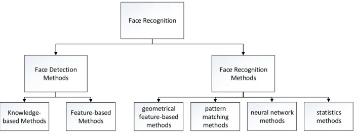
Generally, a face recognition framework is divided into two sequential processes, which are face detection and face recognition. As introduced in the previous chapter, face detection focuses on capturing the face region from the image. Then the face region is delivered to a face recognition process for

verification. The structure of this process is shown in Figure 1.

Face Recognition Face Detection Methods Face Recognition Methods Knowledge-based Methods Feature-based Methods geometrical feature-based methods pattern matching methods neural network methods statistics methods

Figure 1 Face recognition system

2.1.1 Face detection

Face detection is a necessary step in face recognition systems, which localize and extract the face region from the background. Basically, face detection can be classified into two categories, which are knowledge-based methods, and feature-based methods [47].

(17)

8

Knowledge-based methods are actually based on a series of rules generated from researchers’ prior knowledge of human faces, such as the face color distribution, distance or angular relationship between eyes, nose, and mouth. Most of these rules are straightforward and easy to find.

Yang and Huang [21] proposed a layered knowledge-based face detection method in 1994. Their system is consisted of three different levels. At the highest level, the face candidates are found by scanning the input image windows and applying the rule set for each component on face. At the second highest level, the rule set is used for describing what a human face looks like. More prior knowledge is added at this level. The lowest level depends on detailed facial features. The process actually refines the detection process step by step. The reason is that higher step is able to eliminate those images which are not face images, so that the speed of following steps is improved.

Feature-based methods detect face region based on internal facial features as well as the geometrical relationship among them [50]. Contrary to knowledge-based methods, feature-based methods seek constant features as a means of detection. Researchers have proposed a number of methods, which detect face features first, then deduce whether this a real face. Facial features, such as eyebrow, eyes, nose, mouth, and hairline are usually extracted with an edge detector. According to the extracted features, statistical models describing the relationship between each features can be built, so that the face region can be captured. However, feature-based methods are always susceptible to illumination, noise, and occlusion, as these factors seriously damage edges on face [51].

2.1.2 Face Recognition

Face recognition methods can be classified into three categories, which are early geometrical feature-based methods and pattern matching methods, neural network methods, and statistical methods.

The earliest face recognition was based on geometrical features of a face. Simply, the basic idea of this kind of method is to capture the relative position and relative size of representative facial components, such as eyebrows, eyes, nose, and mouth [52]. Then face contour information is included to classify and recognize the faces. Pattern matching methods are the simplest classification methods in the field of pattern recognition. In face recognition, face images in a dataset are treated as the pattern, so once a new image is available, a correlation score between the pattern and the new image can be calculated to generate the final result.

Artificial neural network research dates to the 1940s when Warren McCulloch and Walter Pitts [22] first applied the concept to mathematics and algorithms. The idea of artificial neural networks is inspired by biological neural networks, which consist of a large number of neurons. The neurons in artificial neural networks are actually a group of individual functions, each of which is responsible for a certain

(18)

9

task. The neurons are connected with weighted lines which pre-process the input generated from the previous neuron. The advantages of applying neural network to face recognition are its ability to store distributed data that can be processed in parallel.

The structure of a single neuron is simple with limited functionality; however, an entire neural network consisting of a number of neurons is able to achieve various complicated goals. Furthermore, the most significant feature that neural network possesses is self-adaptability, which means it is able to enhance itself through iteration. The most representative neural network methods in face recognition are multi-level BP networks and RBF networks [53] [54].

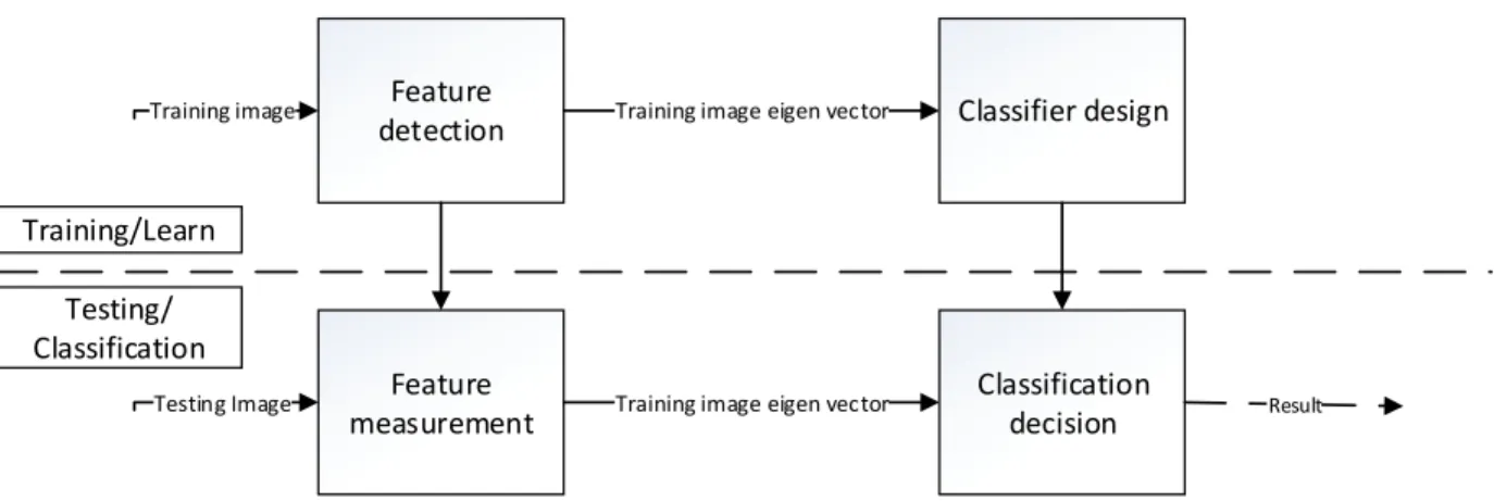
Statistics-based methods attract attention from researchers in face recognition. The idea of a statistics-based method is to capture statistical feature of a face through learning, and then use the acquired knowledge to classify the face. The learn and classification process is shown in Figure 2.

Among all statistics-based methods, subspace analysis is the major type. The basic idea is to compress the face image from a high dimensional space to on with lower dimensions through a linear or non-linear transformation. These methods include Linear Discriminant Analysis (LDA), Independent Component Analysis (ICA), and Principal Component Analysis (PCA).

Feature

detection Classifier design

Feature measurement

Classification decision Training image eigen vector

Training image eigen vector Training image

Testing Image Result

Training/Learn Testing/ Classification

Figure 2 Learning and classification process

2.2 Principal Component Analysis

In computer science, particularly in the context of Big Data, data is often expressed as vectors and matrices. In terms of images, the increase of the resolution of an image means the size of the matrix is larger. Although current computers are powerful enough to process huge amount of data in relatively short time, efficiency still needs to be considered.

(19)

10

Principal component analysis has been widely recognized as an efficient data dimensionality reduction method using a linear transformation [16]. While reducing the data dimensionality, retaining significant information is the basic requirement.

In statistics, mean value, standard deviation, and variance are always used to analyze the distribution and variation of a set of data. These three values can be calculated with Equation (1), (2), (3).

𝑥 =∑𝑛𝑖=1𝑋𝑖 𝑛 (1) 𝑠 = √∑𝑛𝑖=1(𝑋𝑖−𝑋̅)2 𝑛−1 (2) 𝑠2=∑𝑛𝑖=1(𝑋𝑖−𝑋̅)2 𝑛−1 (3)

However, mean value, standard deviation, and variance functions only work for one-dimensional data. In computer science, the data is always multi-dimensional. So a new measurement which conveys a relationship among data of different dimension needs to be included, which is covariance. Normally, covariance is able to describe the relationship between two random variables, as shown in Equation (4).

𝑐𝑜𝑣(𝑋, 𝑌) =∑𝑛𝑖=1(𝑋𝑖−𝑋̅)(𝑌𝑖−𝑌̅)

𝑛−1 (4)

Therefore, as the dimension increases, multiple covariance needs to be calculated, e.g. the number of covariance needed when dealing with n-dimensional data is shown in Equation (5).

𝑛!

(𝑛−2)!×2 (5)

Fortunately, a matrix approach offers a perfect solution for this calculation. The Equation (6) shows the definition of a covariance matrix.

𝐶𝑛×𝑛 = (𝑐𝑖,𝑗, 𝑐𝑖,𝑗= 𝑐𝑜𝑣(𝐷𝑖𝑚𝑖, 𝐷𝑖𝑚𝑗)) (6)

Equation (7) shows the covariance matrix of a dataset with three dimensions {x, y, z}.

𝐶 = (

𝑐𝑜𝑣(𝑥, 𝑥) 𝑐𝑜𝑣(𝑥, 𝑦) 𝑐𝑜𝑣(𝑥, 𝑧) 𝑐𝑜𝑣(𝑦, 𝑥) 𝑐𝑜𝑣(𝑦, 𝑦) 𝑐𝑜𝑣(𝑦, 𝑧) 𝑐𝑜𝑣(𝑧, 𝑥) 𝑐𝑜𝑣(𝑧, 𝑦) 𝑐𝑜𝑣(𝑧, 𝑧)

) (7)

It can be found that covariance matrix is a symmetric matrix, whose diagonal shows the variance of each dimensions.

After generating the covariance matrix, we are able to calculate its eigenvalues and eigenvectors through Equation (8).

(20)

11

𝐴𝛼 = 𝜆𝛼 (8)

Where A stands for the original matrix,𝜆 stands for an eigenvalue of A, and 𝛼 represents the eigenvector according to eigenvalue 𝜆.

Usually eigenvalues are sorted in descending order, which corresponds to the importance of the eigenvector. We can choose how much information to retain. In this case, selecting a good threshold with which useful information is retained, whereas less significant information is removed, becomes important.

2.3 Object-oriented Frameworks

In recent years, software reuse has become a significant technique in software engineering. Traditional methods, such as function or library, provide limited reuse, whereas object-oriented frameworks aim at larger components, such as business units and application domains. Building object-oriented framework can save users countless hours and thousands of dollars in development costs by providing reusable skeletons [55]. Object-oriented framework development plays an increasingly necessary role in contemporary software development. Frameworks like MacApp, ET++, Interviews, ACE, Microsoft’s MFC and DCOM, JavaSoft’s RMI and implementations of OMG’s CORBA are widely used [23].

Some of the features of object-oriented framework are listed below: A. Modularity

Framework enhances software modularity by encapsulating variable implementation details into fixed interfaces. The impact caused by variations of design and implementation is localized by a framework, so that makes software maintenance much easier.

B. Reusability

Framework improves software reusability, as the interfaces provided by a framework are defined as class attributes which can be applied to build new applications. Actually, the reuse of framework takes advantage of the expertise and effort of experienced software developer to minimize the time spent by subsequent developers on the same problem in the domain.

Framework reuse not only improves software productivity, but also enhances the reliability and stability of software.

C. Extendibility

Some frameworks provide hook methods allowing applications to extend their fixed interfaces, so that the extendibility is improved.

(21)

12

2.4 Machine Learning Approaches

Machine learning aims at simulating human activities using computers, so it is able to recognize known knowledge, gain new knowledge with which to improve its performance and optimize itself. Machine learning is being applied to various fields, such as biology, economics, chemistry, and computer science. In 1999, H. Nielsen et al. applied machine learning approaches to prediction of signal peptides and other protein sorting signals [24]. In 2005, CO AIM et al. proposed a method for predicting emotion based on text using machine learning [25]. Companies, such as Amazon, and IBM do research on machine learning as well. Amazon held a machine learning contest to verify whether it was possible to grant and revoke access to employees automatically. Researchers from IBM invented a way to extract heart failure diagnosis criteria from free-text physician notes using machine learning [26].

Generally, machine learning targets four categories of problems, which are regression, classification, clustering, and modeling uncertainty, known as inference.

A. Classification

In classification, input data is divided into different categories. Normally, a classification task belongs to supervised learning, as the categories are labeled. The learning system gains knowledge, with which to assign new input data to one or more of these categories. B. Regression

To some extent, a regression problem is similar to classification, as it is also processed in a supervised way. The most significant difference is the output generated from regression problem is continuous, instead of discrete, like classification.

C. Clustering

Clustering can be regarded as unsupervised version of classification. The basic functionality is also to classify a set of input into different classes; however, in clustering, the categories are not labeled anymore, which means the categories are generated as the system runs.

D. Modeling uncertainty

Modeling uncertainty is not just to predict the frequency of random events. It integrates various factors that affect the occurrence of the event and analyzes the event using mathematical approaches, like Bayesian representation.

The process of establishing a face recognition system is to teach computers to recognize human face as human behavior, i.e. it is a learning procedure. Therefore, machine learning becomes a perfect solution to this problem. According to an evaluation of traditional face recognition techniques and machine learning

(22)

13

approaches by E. Garcia Amaro et al, machine learning generates a better result [56]. In M. S. Bartlett et al’s work, a machine learning algorithm, Adaboost, is combined with SVM, LDA and Gabor filters, which are classical approaches applied to face recognition for building a facial expressions system. The result suggests a mean accuracy of 94.8%, and the system is able to operate in real-time [57].

(23)

14

Chapter 3 Framework for PCA-based Face Recognition

In this chapter, the classical PCA-based face recognition process is presented first, which shows the entire work flow and suggests some common approaches to the process. Then, a software framework for PCA-based face recognition system is proposed. All components contained in the framework are

demonstrated in detail.

3.1 General Requirements

The framework’s target is to provide users with a tool, which is able to help them apply PCA to face recognition applications. Meanwhile, various extreme conditions, such as non-uniform illumination, shooting angle, and facial expressions need to be considered.

The first requirement of the framework is to describe the complete PCA-based face recognition system so that, software developers can use it as a guide to customize their own applications. Therefore, the framework intends to cover as many cases as possible.

Second, the framework needs to be flexible. Hence, each phase in the process needs to include multiple variations in order to deal with different situations. Moreover, the attribute of each variation should be described explicitly, thus making it easier for developers to select. We also mention possible

combinations between different variations for developers’ reference.

Third, the model should be extendable. Since face recognition is still developing rapidly, more

advanced techniques will be proposed to enhance the performance of current systems. The architecture of the framework should allow adjustment or enhancement in the future.

3.2 PCA based Face Recognition Process

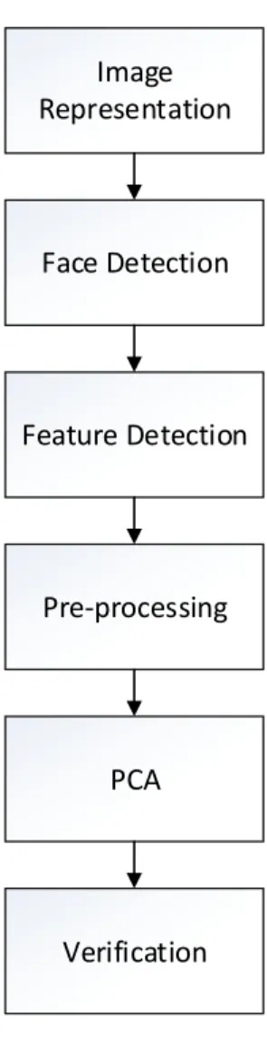
The entire facial recognition process with PCA is shown in Figure 3 and includes 6 main steps: (1) image representation, (2) detecting face regions, (3) detecting facial features, (4) pre-processing, (5) conducting PCA, and (6) verification. Image representation converts the image data to a proper format. Face region detection and facial feature detection prepare meta-data for the following steps. Pre-processing reduces influences caused by the environment such as illumination to exhibit the exact information of the image. Conducting PCA classifies images based on the thresholds set at the verification step.

(24)

15

To verify a face image using PCA, two image datasets are needed: a training dataset providing data for building a customized PCA model, and a testing dataset containing the images to be verified.

Image Representation Face Detection Feature Detection Pre-processing PCA Verification

Figure 3 PCA-based face recognition system flow

3.2.1 Image Representation

Images are stored as a 2-dimensional (2-D) matrix in a computer. Each element in the matrix represents a single pixel whose value ranges from 0 to 255. Color images have 3 different channels which represent red, green and blue, respectively. An extra channel named α represents the transparency of the image. The number of rows and columns of the matrix depends on the resolution of the image, which means that if an image has a higher resolution then there are more rows and columns and more storage is needed.

Moreover, the number of rows and columns significantly affects the matrix computation speed. The size factor leads to a requirement to compress the data, which is why we want to use PCA.

(25)

16

Image representation is not only to minimize the size of an image. Selecting appropriate image representation approaches for different recognition algorithms will improve efficiency and accuracy, which will be discussed in detail in Section 3.3.1.

3.2.2 Face Detection

Face detection extracts the face region from the background of the image. As we can see, this technique has been integrated into most smart phones and works well in most situations. However, an approximate face area might be good enough for smartphone cameras, but when conducting face recognition, slight noise would impact the final result. For an environment where background color is closed to skin color, or part of the face is in shadow, obtaining the face area becomes more difficult.

3.2.3 Feature Detection

To achieve high recognition accuracy using PCA, image alignment has to be performed. An affine transformation is a preferred choice for image alignment, as it is simple and can be processed quickly by a computer. To perform an affine transformation, three feature points are required on the facial image. The pupils of the eyes and the center point of mouth can provide these three points. Thus, the task of this step is to acquire these three feature points from face images

In 2003, Z.Y.Peng, HZ Ai et al., proposed a feature detection method based on weight similarity [5]. First, the algorithm transforms the image to a binary format and the face area can be represented by B(x,y). Equation (9) shows the threshold for the binary image where H(i) stands for the histogram of the original image. Based on the pixel distribution of the face image, approximate areas of left eye and right eye can be measured, which can be represented as L(x,y) and R(x,y) respectively. Since the color of pupils differs from other part of eyes, once a point Pl(x,y) = 1 is found, it can be assumed as left pupil candidate.

Similarly, once a point Pr(x,y) = 1 is found, it can be assumed as right pupil candidate. If both of Pl and Pr

meet the condition shown in Equation (10), they can be confirmed as the center points of two pupils. In the Equation (10), γ(Pl,Pr) stands for the similarity of the neighborhood of Pland Pr, D(Pl,Pr) and A(Pl,Pr)

are the distance constraint and angle constraint of Pl and Pr respectively. After localizing two pupils, the

center point of mouth Pm can be confirmed by integral projection. Figure 4 shows the flow of feature

detection. 𝐵(𝑥, 𝑦) = {0 𝑖𝑓 𝐴(𝑥, 𝑦) ≥ 𝜃 1 𝑖𝑓 𝐴(𝑥, 𝑦) ≤ 𝜃, ∑ 𝐻(𝑖) = 15% × ∑ 𝐻(𝑖) 𝑖=0 255 𝜃 𝑖=0 } (9) 𝐵(𝑥, 𝑦) = 𝒎𝒂𝒙(𝛾(𝑃𝑙, 𝑃𝑟)𝐷(𝑃𝑙, 𝑃𝑟)𝐴(𝑃𝑙, 𝑃𝑟)) (10)

(26)

17

Figure 4 Feature detection [5]

3.2.4 Pre-processing

Image pre-processing is always an important topic in face recognition, since in this step, most factors which potentially affect the final recognition result expect to be eliminated. Researchers have explored a large number of methods to reduce different types of noise, including histogram normalization and converting an image to a binary representation. The majority of these methods aim to reduce noise, whereas some of them also change the format of the image which then can be used in later steps. In this section, we continue the content in feature detection and introduce the basic idea of affine transformation in images.

As we have discussed, three feature points, i.e., two pupils and the center point of mouth can be

represented as Pl, Pr, and Pm. Basically, an affine transformation aligns every image according to the same

template. The three feature points will remain in the same position, and the other pixels will be moved. Equation (11) shows the principal of affine transformation, where (x, y) and (x', y') stand for the pixels on the original face image and transformed template image, respectively.

[𝑥′_𝑦′] = [_𝑎𝑎11 𝑎12 𝑎13 21 𝑎22 𝑎23] [ 𝑥 𝑦 1 ] , [𝑎_𝑎11 𝑎12 21 𝑎22] ≠ 0 (11)

(27)

18 3.2.5 Principal Component Analysis

The concepts behind PCA were invented in 1901 by Karl Pearson [6]. The original idea is to use an orthogonal transformation to convert a set of observations of possibly correlated variables into a set of values of linearly uncorrelated variables called principal components. In 1991, Pentland and Turk

transplanted PCA to face recognition and proposed a method called eigenface, which is frequently used in face recognition research. The basic idea is to extract the most significant information from face images which then can be used to form a sub-space named feature space. The dimensionality of the new formed sub-space is much smaller than that of original images, but components which are used for identifying a face are retained. The image set used to build this sub-space is called a training set, and the image set reflecting the components in the sub-space is called an eigenface. Once the sub-space is established, a testing image can be projected onto the space to generate a new image. The similarity of this new image and the original image can be used for the verification step.

In Equation (12) and (13), M stands for the dimensionality of the feature sub-space, Uk, k = 1,2,...,M are

the eigenfaces, ω stands for the average face.

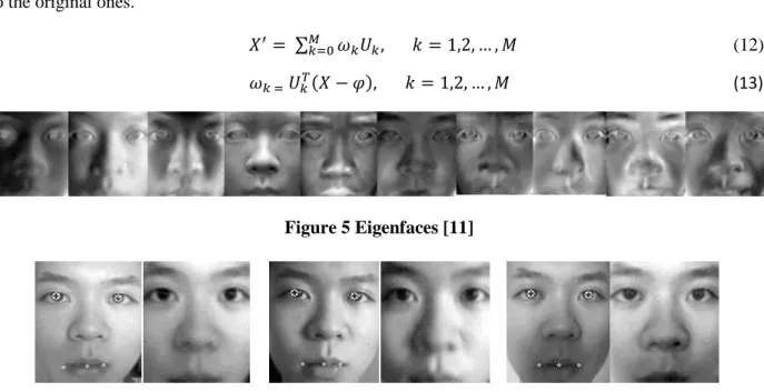
Figure 5 shows a set of eigenfaces generated from a training dataset containing about 200 pictures. Figure 6 shows 3 original pictures and corresponding ones after being projected to the sub-space. As the pictures of the training dataset are of the same person, so the projected pictures are relatively similar to the original ones.

𝑋′ _{= ∑} _𝜔 𝑘𝑈𝑘, 𝑘 = 1,2, … , 𝑀 𝑀 𝑘=0 (12) 𝜔𝑘 = 𝑈𝑘𝑇(𝑋 − 𝜑), 𝑘 = 1,2, … , 𝑀 (13) Figure 5 Eigenfaces [11]

(28)

19 3.2.6 Verification

As already mentioned, the verification step compares the original input image with its projection on the feature sub-space. However, there are many methods for comparing the similarity of two images.

Choosing the proper method can help generate better results.

Since images are represented as a matrix, the problem becomes one of comparing the similarity of two matrices or vectors, which can be easily solved with statistical methods.

Measures such as Euclidean distance, Manhattan distance, Chebyshev distance, and Minkowski distance are all sufficient to tackle such a problem. Each of them has its own advantages and disadvantages, so selecting the optimal measure to for the problem is important.

(29)

20

3.3 Framework model

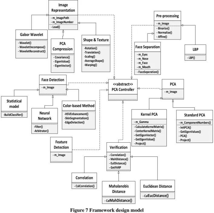
In this section, a framework for a face recognition system with PCA is presented, as shown in Figure 7. The framework describes the entire recognition process, and for each phase in the process, some possible variations are offered to adapt to different cases and to help software developers customize their

application. Some extreme cases, such as non-uniform illumination, exaggerated facial expression, shooting angle of the images, and data type of the images are considered. Besides the options included in the framework, we suggest other potential approaches. The outline of the framework follows.

For face representation, we will talk about Gabor wavelet, PCA expression, and shape and texture expression. For face detection, we will talk about statistical model, neural networks, and color based methods. For pre-processing, we will talk about face separation, and local binary pattern (LBP). For PCA, which is the core step, we will talk about Kernel PCA and standard PCA.

Through the combination of different variations, the framework is able to provide at least 108 application instances in total, as there are three variations for face recognition step, face detection step, and verification step respectively, and two variations for pre-processing step and PCA step respectively. However, the application instances which can be produced by the framework is a lot more than 108, since in practical use, some variations in the same step might be combined, some steps can be omitted, and some variations need to collaborate with other simple mathematical operations. Therefore, a conservative estimate of the actual number of application instances that can be produced by this framework exceeds 150. Though these instances are not able to cover all situations, the framework offers a significant assistance to software developers.

(30)

21 <<abstract>> PCA Controller Image Representation - m_ImagePath - m_ImageNumber - Load() Gabor Wavelet - Wavelet() - WaveletDecompose() - WaveletReconstruct() PCA Compression - Covariance() - EigenValue() - EigenVector()

Shape & Texture

-Rotation() -Translation() -Scaling() -AverageShape() -Warping() Face Detection - m_Image Statistical model -BuildClassifier() Neural Network -Filter() -Arbitrator() Color-based Method -HSVEnhancement() -SkinSegmentation() -EdgeDetection() Feature Detection - m_Image Pre-processing - m_Image - Binarize() - Normalize() - Affine() Face Separation - m_Eyes - m_Nose - m_Face - m_Mouth - FaceSeperation() LBP - LBP() PCA - m_Image Kernel PCA - m_Gamma - CalculateKernelMatrix() - CenterKernelMatrix() - GetEigenVector() - GetEigenValue() - Project() Standard PCA - m_ComponentNumbers() - InitPCA() - GetEigenValues() - PCA() - Project() Verification - Correlation() - MahDistance() - EulDistance() - GetFARP Correlation - CalCorrelation() Mahalanobis Distance - CalMahDistance() Euclidean Distance - CalEucDistance()

Figure 7 Framework design model

3.3.1 Image Representation

As the first processing step of face recognition, image representation playes an important role not only in explicitly representing the image information, but reducing noise and compressing data. Appropriate selection of image representation approaches facilitates the later steps and improves the overall

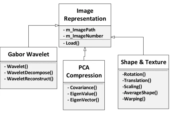
performance of the entire system. In this section, we present three different variations for representing images, which are Gabor Wavelet, PCA Compression and Shape and Texture, as shown in Figure 8.

(31)

22

Image

Representation

- m_ImagePath

- m_ImageNumber

- Load()

Gabor Wavelet

- Wavelet()

- WaveletDecompose()

- WaveletReconstruct()

PCA

Compression

- Covariance()

- EigenValue()

- EigenVector()

Shape & Texture

-Rotation()

-Translation()

-Scaling()

-AverageShape()

-Warping()

Figure 8 Image representation

3.3.1.1 Gabor Wavelet

Image processing methods are mainly divided into two categories, which are spatial domain analysis and frequency domain analysis. Spatial domain analysis directly processes the image matrix; however, frequency domain approaches convert the image from the spatial domain to the frequency domain, and then analyze the image feature from another perspective. Spatial domain analysis is widely used in image reinforcement, image reconstruction, and image compression [25].

Fourier transforms are one of the earliest method of transferring signals from the spatial domain to the frequency domain, as shown in Equation (14). After processing the signal, an inverse transform can transfer the signal back to spatial domain through Equation (15).

𝐹(𝜔) = ∫∞ 𝑓(𝑡)𝑒−𝑗𝜔𝑡_{𝑑𝑡 = 𝐹[𝑓(𝑡)]} −∞ (14) 𝑓(𝑡) = 1 2𝜋∫ 𝐹(𝜔)𝑒 −𝑗𝜔𝑡_{𝑑𝜔 = 𝐹}−1_[𝑓(𝑡)] ∞ −∞ (15)

Classic Fourier transform provides a powerful tool for image processing; however, it is only able to reflect the integral attributes of signals, which means it lacks the ability to do local analysis.

Based on Fourier transform, Dennis Gabor proposed a new transform which only depends on part of the signal and is able to extract local information, [45].

(32)

23

The basic idea of the Gabor transform is to divide the signal into multiple intervals, and then analyze each interval using a Fourier transform, so that the frequency in certain interval can be obtained. In image processing, a Gabor transform is also known as Gabor wavelet.

A Gabor wavelet is similar to the stimulation of a simple cell in a human being’s visual system [28]. It captures salient visual properties such as spatial localization, orientation selectivity, and spatial frequency. Furthermore, as Gabor wavelet is insensitive to illumination variation, it provides good adaptability to illumination variation in image representation.

It has been proved that the Gabor wavelet is particularly suitable for image decomposition and representation when the goal is the derivation of local and discriminating features. In 1999, Donato et al. [7] showed that the Gabor filter representation gave better performance for classifying facial actions. In 2001, Chengjun and et al. [29] presented an independent Gabor feature method for face recognition. The method achieved 98.5% correct face recognition accuracy on FERET dataset, and 100% accuracy on ORL dataset.

3.3.1.2 PCA Compression

As the core of this study, PCA is the main step of a face recognition system that we discuss. However, it also can be used as an image representation method when combining with other recognizing

approaches. When representing face image using PCA, the main idea is to transfer the original image to a format with lower dimensions, i.e., to represent by a smaller number of parameters.

PCA was first applied to the realm of pattern recognition in 1965 by Watanabe [30]. In 1990, Kirby et al. introduced the method to face recognition, particularly characterization of human faces [31]. The work introduces a concept of optimal coordinate system, in which the set of basis vectors which makes up the system are referred to as eigen-pictures. They are actually the eigenfunctions of the covariance matrix of the ensemble of faces. For the evaluation of the procedure, face images from outside of the dataset are projected on the set of optimal basis vectors. The result shows a 3.68 percent error rate out of over ten face images, which dominated in this field at the time.

As the development of face recognition technique evolves, some variations of PCA-based image representation method have been invented. Moreover, PCA-based image representation is always combined with other recognition approaches to achieve better recognition accuracy.

In 2005, Daoqiang and Zhi-Hua proposed a two-directional two dimensional PCA for face

representation and recognition [32]. It has been proved that 2DPCA outperforms standard PCA in terms of recognition accuracy. However, 2DPCA needs more coefficients for image presentation than PCA.

(33)

24

Therefore, Daoqiang and Zhi-Hua conduct PCA on row and column directions simultaneously, which results in a same or even higher recognition accuracy than 2DPCA, though with less coefficients needed.

3.3.1.3 Shape and Texture Expression

Shape and texture expression methods uses geometric features to represent a human face. As shape and texture expressions ignore the color and illumination of a face, it reduces the noise that impacts the recognition accuracy. In fact, shape-based and texture based methods were independent initially. After proving that the shape-based method cannot perfectly solve the problem caused by expression, scale and illumination, texture is introduced to be combined with shape to achieve better recognition accuracy [32].

Chengjun Liu and Harry Wechsler’s paper in 2001 [8] clearly explains the work flow of shape and texture-based face expression methods. We use some of the figures and explanations to demonstrate the principle in detail.

The shape of face images reflects the contours of face, so a set of control points derived by manual annotation are used to describe the contour. To underscore the shape features of face, these points ignore other facial information like color, gray scale. They only depict feature points such as eyebrows, eyes, nose mouth, and the contour of face, as shown in Figure 9. Generally, the shape image is generated from a large set of training images. After obtaining the shape from each training image, the shapes are aligned by rotation, translation and scaling transformations. The aligned shapes of training images are shown in Figure 10.

Calculating the average of the aligned shapes of training images, a mean shape can be obtained. Then warp the normalized (shape-free) face image to the mean image, a new image is created, which is the texture, as shown in Figure 11. The warping transformation basically separated the image into multiple small triangular regions and then performs affine transformation on each of them to warp the original face to the mean shape. These two steps will result in a texture (shape-free image) which has the same face contour as the mean shape.

The experimental result of Chengjun Liu and Harry Wechsler’s work shows that the integrated shape and texture features capture the most discriminating information of a face, which contributes to their high recognizing accuracy. Besides their work, other research [34] [35] [36] demonstrate the advantages of using shape and texture method to represent facial image.

(34)

25

Figure 9 Control points [8]

(35)

26

Figure 11 Texture [8]

3.3.2 Face Detection

Face detection provides the basic face area image for the entire recognition process. The detection accuracy significantly influences the final result, as too much background noise affects most recognition algorithms. For this phase, we provide three variations, which are the statistical model, Neural Network, and color-based method, as shown in Figure 12.

Face Detection

- m_Image

Statistical model

-BuildClassifier()

Neural Network

-Filter()

-Arbitrator()

Color-based

Method

-HSVEnhancement()

-SkinSegmentation()

-EdgeDetection()

Figure 12 Face detection

3.3.2.1 Statistical Model

The complexity of human face images makes the detection of face features to be difficult, therefore statistical-based detection methods have been attracting researchers’ attention. This method regards the face region as a type of pattern, also known as pattern feature, and uses a large number of face image and non-face image to train and generate a classifier. So the more training the detection method receives, the more robust it will be.

Feature space-based methods, such as PCA, LDA, probabilistic model-based methods, and support vector machine-based (SVM) methods all belong to statistics-based detection methods. Actually, neural networks-based methods, which are discussed next also utilize statistical principles; however, we explain it individually because of some of its peculiarities.

(36)

27

In 2000, Henry et al. [9] proposed a statistical method for 3D object detection. The method is able to detect both object appearance and “non-object” appearance using the product of histograms. Each

histogram represents the joint statistics of a subset of wavelet coefficients and their position on the object. The approach uses many such histograms that represent a wide variety of visual attributes. The result demonstrates detection accuracy.

In 1997, Baback Moghaddam and Alex Pentland proposed a probabilistic visual learning for object representation, which is based on density estimation in high-dimensional spaces using an eigenspace decomposition [37]. The technique has been applied to not only face detection, but gesture recognition.

3.3.2.2 Artificial Neural Network

An Artificial Neural Network is a computation model consisting of many neurons, in which each neuron includes a specific output function called an activation function. The connection between every two neurons has a weight that processes the output from the first neuron.

The most significant attributes of artificial neural networks are their adaptability and parallelism. Adaptability grants its ability to learn through training and autonomously correct weights in connections to avoid the same faults. As each neuron in the network is responsible for a certain job, an artificial neural network is able to work in parallell, which facilitates processing big data such as images.

Because of these two remarkable attributes, artifical neural networks have been attracting attention from researchers in face recognition. In 1997, Shang-hung et al. proposed a face detection method using a probabilistic decision-based neural network. The detection accuracy reaches 98.34%. In 1998, Henry et al. [10] presented a neural network-based upright frontal face detection system. Figure 13 shows the basic idea of the system. A window of the image which might contain a face region is first obtained. Then a series of pre-processing steps, such as light correction and histogram normalization, are applied to the window to reduce noise. Finally, the window is passed through a neural network, which decides whether the window contains a face. It has been shown in the result that the algorithm can detect between 77.9 percent and 90.3 percent of faces in a set of 130 test images, with an acceptable number of false positives.

(37)

28

Figure 13 Artificial neural network-based method [10]

3.3.2.3 Color-based Methods

Traditional face detection approaches are always performed in gray-scale space, in which the gray-scale is the only information that can be captured. Moreover, since there is no limit for area or proportion, it is necessary to search the entire space, which is fairly time-consuming. However, if color information can be introduced, the search area will be narrowed, because the skin color is the most straightforward information on a human face. In addition, in the face region, skin color dominates.

A problem that needs to be considered is the difference of skin color. Fortunately, research in this field shows that skin color in certain color space aggregates, especially when the illumination factor is removed [46]. Therefore, using skin color as a clue to exclude any area which is not skin can be easily performed.

When applied to face detection, skin color information is always used in three different phases of face detection. It could be used as the core function, the pre-processing method, or in post-verification. For instance, in 2002, Hichem Sahbi and Nozha Boujemaa proposed a skin color approach for face detection combined with image segmentation. In their approach, the images are first separated coarsely to provide regions of homogeneous statistical color distribution. Then the color distribution will be used for training a neural network to detect faces. The experiment result shows an accuracy of around 90%.

3.3.3 Pre-processing

A pre-processing step can be regarded as a filter which reduces major noise impacting the following recognition process. It aims at generating clear images with useful information retained. As shown in Figure 14, this section discusses two pre-processing approaches, which are face separation and LBP. Face separation mainly handles face images with exaggerated expressions, and local binary patterns deal with non-uniform illumination.

(38)

29

Pre-processing

- m_Image

- Binarize()

- Normalize()

- Affine()

Face Separation

- m_Eyes

- m_Nose

- m_Face

- m_Mouth

- FaceSeperation()

LBP

- LBP()

Figure 14 Pre-processing 3.3.3.1 Face Separation

When people take pictures, it is hard to always control their facial expressions. On the other hand, as an ideal face recognition system, it should not be expected that subjects will have normal expressions. However, extremely exaggerated facial expressions do impact the recognition process, especially for feature detection or image aligning. To reduce the influence, this pre-processing method divides a face image into 4 parts which are: eyes, nose, mouth, and entire face, so the following steps can be performed on each part, as shown in Figure 15.

Figure 15 Face separation [11]

In 2014, Peng et al., used face separation for standard PCA-based face recognition system [11]. They conducted PCA on each part of the face mentioned previously, and integrated the score with Equation (16), where 𝛿𝐹 stands for the score of entire face, 𝛿𝑀stands for the score of mouth, 𝛿𝑁stands for the

(39)

30

experimentation. The result shows significant progress in recognizing face images with exaggerated expressions.

𝛿 = 0.40 × 𝛿𝐹 + 0.10 × 𝛿𝑀+ 0.10 × 𝛿𝑁+ 0.40 × 𝛿𝐸 (16)

3.3.3.2 Local binary pattern

Local binary pattern, known as LBP, was proposed by D.C. He and L. Wang in 1990 [12]. The basic idea is to calculate a weighted sum for a single pixel with it neighboring pixels. Generally, the window size of sum is set as 3×3. Basically, it is still creating a binary representation of an image. LBP traverses the image using every pixel as a center point, and for all of the eight neighboring pixels, a calculation is performed. If a pixel has a gray value less than the gray value of the center point, assign the pixel a value of zero; otherwise, assign one, as shown in Equation 17 and Figure 16, where 𝐼(𝑍𝑖) represents

neighboring pixels, and 𝐼(𝑍0) represents the center pixel. The assignment process can be demonstrated by

Figure 16. The weight assigned to each pixel is always different. One possible weight distribution is shown in Figure 17. Figure 18 shows an image which is processed by LBP.

𝑓(𝐼(𝑍0), 𝐼(𝑍𝑖)) = { 0, 𝑖𝑓(𝐼(𝑍𝑖) − 𝐼(𝑍0) > 0) 1, 𝑖𝑓(𝐼(𝑍𝑖) − 𝐼(𝑍0) < 0) , 𝑖 = 1,2,3, … ,8 (17) Figure 16 LBP Figure 17 LBP weight

(40)

31

Figure 18 LBP result [11]

It has been shown that LBP performs well on image classification, and as the computation is simple, it is efficient for most cases. However, it has some limitations including low extendibility and scalability.

Fortunately, after about 10 years of research, some variations of LBP have partially overcome these deficiencies. In 2002, Ojala T. et al. [13], proposed a method which uses a circular neighborhood with arbitrary radius instead of a 3×3 window, as shown in Figure 18. In 2007, Xiaoyang Tan et al. [14], made changes based on LBP and proposed Local Ternary Patterns (LTP), which compares the value of

neighbor pixels with the value of the center pixel plus a range value t. Then the eight neighbor values are able to be encoded. The process is shown in Figure 19. Besides the variations of LBP, researchers also combined LBP with other algorithms, in order to enhance the efficiency.

Figure 19 Circle LBP

(41)

32 3.3.4 PCA

In this section, the core step, using PCA for recognition of face images is discussed. As the Figure 21 shows, two variations are provided. Standard PCA is mainly used for linear image data, whereas kernel PCA is used for non-linear image data. The source of the figures in this section can be found at [39].

PCA

- m_Image

Kernel PCA

- m_Gamma

- CalculateKernelMatrix()

- CenterKernelMatrix()

- GetEigenVector()

- GetEigenValue()

- Project()

Standard PCA

- m_ComponentNumbers()

- InitPCA()

- GetEigenValues()

- PCA()

- Project()

Figure 21 PCA 3.3.4.1 Standard PCA

A common application of PCA is to reduce the dimensions of the dataset with minimal loss of information. Here, the entire dataset (d dimensions) is projected onto a new subspace (k dimensions where k << d).

The standard PCA approach can be summarized as six simple steps [15]: 1. Compute the covariance matrix of the original d-dimensional dataset X. 2. Compute the eigenvectors and eigenvalues of the dataset.

3. Sort the eigenvalues by decreasing order.

4. Choose the k eigenvectors that correspond to the k largest eigenvalues where k is the number of dimensions for the new feature subspace.

5. Construct the projection matrix W of the k selected eigenvectors.

(42)

33

Figures 22, 23, and 24 show an example of using PCA on a dataset with the dimensionality of three. Figure 22 shows the original dataset. Two categories of data are mixed together and hard to be classified. Figure 23 shows the eigenvalues and eigenvectors of the original dataset. After being processed by PCA, the dimensionality is reduced to 2 and the classification is clearer, as shown in Figure 24.

Figure 22 Original dataset [39]

(43)

34

Figure 24 Classification by using standard PCA [39]

The original idea of using PCA on face recognition was first proposed by Turk and Pentland in 1991 [16]. The basic principle has been introduced in previous sections. Although researchers have been studying PCA for decades, it is still a preferred approach for face recognition, because of its robust nature and extendibility. In addition, it is easy to combine PCA with other existing methods.

3.3.4.2 Kernel PCA

Kernel PCA is an extension of PCA using techniques of kernel methods. The basic idea is to first map the input space into a feature space via nonlinear mapping and then compute the principal components in that feature space.

Standard PCA works well if the data is linearly separable. However, in practice, image data is always impacted by external factors, such as shooting angle, illumination, and other noise. So the property of being linearly seperable is not guaranteed. Hence, a method dealing with nonlinear cases is required. Figure 25 shows a comparison between linear data and non-linear data.

(44)

35

There are 2 main steps in the implementation of kernel PCA: 1. Computation of the kernel (similarity) matrix. 2. Eigen decomposition of the kernel matrix.

Figure 26, 27, 28, and 29 show an example using standard PCA and the Gaussian radial basis function (RBF) kernel PCA on a nonlinear dataset. Figure 26 and Figure 28 show the distribution of data. Figure27 and Figure 29 are the corresponding results. It can be clearly seen that the projection via RBF kernel PCA yielded a subspace where the classes are well separated.

Figure 26 Original data [39]

(45)

36

Figure 28 Original data [39]

Figure 29 Kernel PCA result [39]

3.3.5 Verification

As shown in Figure 30, we introduce three measurements for the final verification step. The methods in this step are basically mathematical formulae related to matrix operations, as the verification step is actually comparing the results represented as a matrix from previous steps. The three methods are correlation, Mahalanobis distance, and Euclidean distance.

A Software Framework for PCA-based Face Recognition