FAST SUPERRESOLUTION BASED ON A NETWORK STRUCTURE
TRAINED USING SPARSE CODING
BY
AHSAN KHALID GHAURI
THESIS
Submitted in partial fulfillment of the requirements
for the degree of Master of Science in Electrical and Computer Engineering
in the Graduate College of the
University of Illinois at Urbana-Champaign, 2012
Urbana, Illinois
Adviser:
ii
Abstract
In this thesis I present a novel approach to superresolution using a network structure. Sparse representation of image signals forms the cornerstone of our approach and the goal is to obtain resolution enhancement of the low resolution images. I will discuss various dictionary learning methods and also a joint dictionary training approach. Superresolution is used to enhance the resolution of low quality and low resolution images from electronic devices such as surveillance cameras, which have limitations on the number of sensors they can accommodate. Many medical diagnostic devices and military applications demand increased image resolution for a better and a more detailed analysis and a deeper understanding of the minute and subtle details. These details are rendered incomprehensible in their original low resolution form. Sparse coding is a technique of finding an optimal sparse code vector corresponding to an input vector. This sparse representation minimizes the error energy function that includes the square of the L2 norm and a regularization term containing the L1 norm of the sparse vector. This sets up a regularized least squares solution. The L1 norm is preferred because it promotes the sparseness of the solution. The L0 norm term in the regularization parameter may result in the solution being obtained in a combinatorial manner, and that may result in finding the solution of the problem to be NP-hard. The regularization term can have an L2 norm, which is called the Tikhonov regularization. The Learning of the Iterative Shrinkage and Thresholding Algorithm (ISTA) is achieved by learning a regression function which accepts a test signal vector as the input and provides a corresponding sparse vector as an output for that signal. The testing part is based on the forward-propagation which is similar to the ISTA network structure. The learning part of the network encoder is however based on a back-propagation model and uses the stochastic-gradient descent method. The error function is the difference between the sparse representations obtained from either ISTA, the Basis Pursuit, or any other L1 regularization solver such as LASSO or LARS, and the regression function obtained by training on the sparse vector obtained from the sparse recovery algorithm. The error function is minimized with respect to the three network parameters. We learn regression function parameters such that the error difference between the regression function and the sparse coding solution vector obtained from the optimization solver is minimized. The sparse representation can also be originally obtained from any convenient L1 regularization solver. Once the regression function is learned, the high resolution patches are simply the product of the high resolution dictionary and the sparse solution obtained from the trained regression function. The low resolution and high resolution
iii
dictionaries are usually trained jointly so the sparse coded solution is the same for both the low resolution and high resolution image patches. Our approach increases the computational speed and tries to decrease its cost as, having learned the regression function, we try to bypass the optimization problem.
iv
Acknowledgments
I would like to express my deepest gratitude to my adviser, Professor Thomas Huang, for giving me the liberty to work on a topic of my interest. My adviser has been very kind and encouraging throughout the process. I would also like to thank my mentor and former group fellow and now post-doctoral researcher in Professor Huang’s wonderful research group, Dr. Jianchao Yang, who has helped me a lot with his ideas and set the goals of this project. He has guided me through the process. I am deeply indebted for the support, both moral and academic, that has been provided by Professor Huang and Dr. Yang.
v
Contents
1 Introduction ... 1
1.1 Sparse Coding ... 1
1.1.1 Regularization ... 2
1.1.2 Sparse Coding Applications ... 4
1.1.3 Online Dictionary Learning for Sparse Coding ... 9
1.2 Superresolution ... 11
1.2.1 Approaches to Superresolution ... 12
1.2.2 Sparse Solvers ... 13
2 Related Work... 19
2.1 Goal of Superresolution ... 20
2.1.1 Dictionary Learning Techniques ... 21
2.1.2 OMP and Batch-OMP ... 22
2.2 The K-SVD Algorithm ... 25
2.2.1 Approximate K-SVD ... 27
3 Our Superresolution Approach ... 32
3.1 Two-Step Dictionary Training for Superresolution ... 32
3.2 Our Motivation ... 34
3.3 Learning the Network Structure for Superresolution ... 34
3.3.1 Learning Function ... 36
3.3.2 Learning Output Weight Parameter ... 39
3.3.3 The Complete Learning Algorithm ... 39
3.4 Discussion ... 39
4 Experiments and Results ... 41
4.1 Training Set Preparation ... 41
4.2 Comparisons with Exact Sparse Recovery Algorithm ... 41
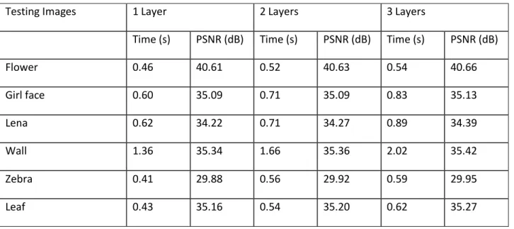
4.3 Effects of Different Network Layers... 44
4.4 Summary ... 44
5 Conclusion and Future Work ... 48
1
1 Introduction
Numerous engineering and signal and image processing tasks involve solving the inverse linear problem. This inverse linear problem can be represented as a system of linear equations.
w
Ax
y
(1.1)Here
A
R
mxn,y
R
n andw
R
mwhere the size ofm
is usually much larger thann
. Thus we can say thatA
is a “fat” matrix with more columns than rows. The termy
is the known vector and is equal to the matrix-vector product ofA
andx
,
whereasw
is the noise vector. The termx
is the unknown solution vector that needs to be determined. Solving this system of equations is computationally difficult because it is underdetermined as the number of unknowns (the number of columns) is much greater than the number of constraints (the number of rows). Thus the matrixA
is overcomplete. Many image processing problems including deblurring and resolution enhancement involve the use of linear inverse problems.1.1
Sparse Coding
The linear system of equations mentioned above usually has a solution
x
which is nonunique because of the fact that the matrixA
is not square and is usually a fat matrix, meaning that there could be infinitely many solutions to this particular system of equations. In fact, the system solution may not even exist. If the matrixA
is ill-conditioned or near singular, then the condition number of the system of equations will be very high, the norm of the solution vectorx
will be large, and the solution will have much less stability, to the extent that it can be very sensitive to perturbations in the input values. The most common approach to solving problems that involve the linear inverse systems of an ill-conditioned nature is to solve the least squares problem. This is done to minimize the L2 norm of the error residual, the formulation of which is described as2
||
||
Ax
b
(1.2)The least squares approach minimizes the square of error between the matrix-vector product and the vector on the left-hand side of the system of equations. It is basically the L2 norm or the Euclidean norm
2
of the error. However, the use of the square of the L2 norm has many limitations in that it does not help in improving the conditioning of the solution vector and the solution is not better than for the case mentioned in Equation 1.1.
1.1.1 Regularization
There is a need to tailor the solution to the system of underdetermined equations such that the solution remains as close as possible to the original system but with some added features. The goal is to have a solution that has a set of particular characteristics and at the same time is not very far off from the original set of values. This is to make sure that the original values of the solution are preserved as much as possible but with some added desirable features.
One particular type of regularization is the Tikhonov regularization in which a Tikhonov matrix
is included in the regularization parameter term. The Tikhonov matrix is included in the regularization term of the minimization process as follows:2 2
||
||
||
||
Ax
b
x
(1.3)In most of the applications that employ the regularization technique, the Tikhonov matrix is the identity matrix. In that case, we are trying to ensure that the solution norm is as low as possible, by enforcing the matrix to be of the minimum norm possible; hence, we are giving preference to solutions with smaller norms.
The level of regularization can be controlled by varying the strength of the regularization parameter. It is usually a convention that the value of the coefficient of the regularization parameter can vary from 0 to ∞. The solution to the regularized least squares problem contains the term which tries to make the inverse of the system as non-singular as possible. The solution to the regularization based least squares problem defined in Equation 1.3 is of the following form:
b A A A x T T 1 T ^ ) ( (1.4)
The coefficient (
or
) of the regularization parameter is essentially the scale of the regularization matrix
. Thus if the coefficient is 0, then we can see from the equation that the solution will simply be the solution to the un-regularized least squares problem, with the condition that(
A
TA
)
1exists.3
When the number of equations is less than the number of variables or the number of unknowns, we usually need to add some constraints so as to obtain a feasible solution. The use of constraints can be either quadratic or linear depending on the applicability. There is, most of the time, a need to solve the constraint problem using a solver. The solver helps in providing a solution to an optimization problem, which is difficult to solve by analytic means. There are some problems that need to be changed from constrained problems to non-constrained problems. The use of Lagrange multipliers helps in changing the problem format from a constrained inequality to a constrained equality. In doing so, we are changing the problem from a constrained to an unconstrained optimization.
There are some algorithms that can be used to change a regularized problem to a standard unconstrained linear or quadratic optimization problem (QP) that can be solved analytically and in a more efficient manner. One such algorithm is the feature-sign search algorithm.
Image processing problems usually require some non-smooth pre-conditioners and regularization terms. The use of L2 norm of the regularization term results in a smoothed out function. Even though the solution space for the L2 norm is the biggest and the computation is somewhat easier, it does not provide a sparse solution.
In order to ensure sparsity in the solution to the least squares problem, we enforce the L1 norm term in the regularization problem. Thus we have an optimization problem that can be solved by using linear solvers. The general problem can be represented in a generic manner:
1 2 2 || || || || min arg Ax b x x
(1.5)The optimization function consists of two parts: the objective function and the regularization term. The goal is to minimize the objective function by minimizing the L2 norm of the square of the error. There is, however, a need to have a compromise between the size of the error residual and the level of sparsity that needs to be imposed to ensure that our solution is meeting both the restrictions at the same time. This compromise involves a trade-off that is controlled by a regularization parameter whose value can vary anywhere from 0 to infinity. If the regularization parameter is 0, then we have a problem in which all we need is to solve the linear problem. If the value of the regularization parameter is too high, then the solution may be highly sparse, but the error residual may be so large as to make the solution inaccurate. In fact, the solution can be erroneous and outside the acceptable range of approximate solutions.
4 1.1.2 Sparse Coding Applications
Image denoising has been studied in great detail in recent decades. The work reported in [1] addresses the image denoising problem. A sparse and redundant representation is applied over a trained dictionary. The denoising and the training of the dictionary using K-SVD over the noisy image content take place simultaneously. Here again, the Bayesian approach is used for the purpose of denoising. This implies that there is a need for an image prior. The image prior in this case is the one that forces sparsity on the entire image. Hence the sparsity is imposed on the image patches in every possible location including the prospect of overlaps of the patches. This global prior is necessary as it ensures the use of images of any arbitrary size. The dictionary training is usually bound to handle image patches of very small size. These correspond to patch vectors of small dimensions. The global image prior is thus the need of the hour to accommodate images of diverse spectrum of sizes. There have been several other research methods whereby local priors have been transformed to a global prior. The work in [2]changes the local Markov random field (MRF) prior into a global prior. The authors have set up a maximum a-posteriori probability (MAP) estimator which minimizes the well-defined global penalty term. The solution obtained is an iterated patch-wise sparse coding. Hence each image block undergoes a sparse decomposition over an over-complete dictionary. The calculation of the average is done afterwards. The contents of the training dictionary are the patches of the noisy image.
The fact that natural signals such as images can be represented as a sparse decomposition of signals over a redundant dictionary has spawned great interest in setting up algorithms for solving such signals. The K-SVD presented in [3] is one such well-defined dictionary learning method for grayscale image processing. The authors of [4]present the dictionary learning problem for colored images and use the K-SVD method for the learning of such dictionaries. In addition to learning of dictionaries for color images, many other signal processing tasks can be performed using the idea proposed by the researchers. The non-homogeneous noise and missing information can be easily handled. The applications include color image de-noising, in-painting and demosaicing. The goal is to implement and extend the de-noising and other applications to the case of color images by simply concatenating the RGB values to form a single vector. The training of the dictionary is then done on this vector directly rather than denoising each channel separately using separate learning and training. There are, however, some drawbacks of color image processing, like false colors and artifacts. The authors of [4] also present the extension of denoising to deal robustly with non-homogeneous noise. The missing values in the image can be
5
modeled as being corrupted by strong impulse noise. The results generated in this work have proven to perform well with state-of-the art results in the denoising, demosaicing and inpainting applications. The most common model for sparse coding is based on Gaussian noise models. A slightly different variation of this Gaussian based noise model is presented in [5]. They call their model the exponential family sparse coding to differentiate from the Gaussian sparse coding. The sparse coding problem is an unsupervised learning in nature. Even then, it has been applied successfully in self-taught learning where the unsupervised and unlabeled data is used to learn a supervised task, even if the unlabeled data has no apparent relation with the labels of the supervised task. The sparse coding and representation problem solves a Gaussian noise model and the squared error in the form of quadratic loss function and is thus not very good in terms of performance, when it comes to binary data or integer valued data. It also does not fare well for any data which is non-Gaussian in nature, for example text based data. The authors seek inspiration from generalized linear models (GLMs) whereby sparse coding is generalized to learn from using the data that is drawn from sources that are different from the Gaussian distribution; the reliance being mainly on any exponential family distribution of data such as Bernoulli, Poisson or even exponential distribution etc. Thus there is an efficient way to model data that is strictly not Gaussian. Thus the model performs exceptionally well as long as the optimal solution is sparse. The authors claim that the results of self-taught learning are improved if the generalized model is applied to text classification based data and robotic perception tasks. The generalization model proposed by the authors makes the self-taught parameter much harder to solve. This can however be solved using the repeated application of a series of L1 regularized least squares problems. The L1 regularized least squares problem can be solved using solver algorithms used to solve the Gaussian sparse coding.
Sparse coding also finds applications in image de-blurring. The authors of [6] propose a deblurring algorithm that utilizes the sparsity and sparse characteristics of natural images. The backward diffusion problem is an ill-conditioned problem. The fundamental point to note in this algorithm is that the sparse code coefficients used to encode a given image with respect to an over-complete basis are the same as the sparse code coefficients used to encode the blurred image of the same original image. However, the basis is slightly modified. Thus the dictionaries may be different but the sparse coefficients of the image representations are the same. The generative model entails the calculation of the sparse coefficients of the blurred image (which happen to be the same as the sparse coefficients of the original image), and these coefficients are combined with the over-complete basis of the original image to get back the
de-6
blurred original image. The generative model in this algorithm fares well against variation methods and fixed basis wavelet methods. Blurring is essentially the convolution of the kernel with the original image. The value of the convolutional kernel is a function of the size of aperture. The net measured image is the blurred form of the ideal focused original image convolved with the point spread function. Blurring is an ill-posed problem and the sensitivity to perturbation and artifacts can be overcome by regularizers like the Tikhonov regularizer. The deblurring method of the authors is novel in that the regularizer uses the sparse natural statistics of the image. Secondly, the ill-conditioning associated with solving an inverse partial differential equation can be avoided.
Sparse modeling of input data has many applications in image processing. Some of the salient applications include image resolution enhancement (also called super-resolution), image denoising, image deblurring, image inpainting, supervised learning and object recognition based on image classification. Researchers in [7] use structured sparse coding for object classification. The subgroups are learned by first dividing the input space in a binary decision tree-like structure. The dictionary is learned and the specified dictionary elements are assigned to each tree leaf. There is a lookup table to store the pseudo-inverses and the assignments of each node of the tree. Thus the authors claim a much more efficient inference. The performance of the algorithm in terms of object recognition inference is state of the art and falls under the category of almost real time inference. In the inference step of the algorithm, the input data is divided into leaves and the set of leaves of the trees are input to a group of pre-specified dictionary atoms. The sparse coefficients thus are obtained with the help of cached pseudo-inverse calculated for each node.
Sparse coding also finds extensive use in face expression classification and recognition. The work done in [8]explores image classification using spatial pyramid matching and sparse coding. The database used is JAFFE, which has a huge dataset for facial expressions. The JAFFE database is rich as it consists of a diverse range of emotions and facial expressions. The seven facial expressions are happy, sad, fearful, angry, disgusted, surprised and neutral. This database is the choice of many researchers in facial expression classification. Facial expression recognition consists of two stages: feature extraction and expression classification. The principal component analysis (PCA), Gabor filter, independent component analysis (ICA), linear discriminant analysis (LDA), support vector machine (SVM) and hidden Markov models (HMM) are the most common choice for feature extraction. The bag-of-features [9] and spatial pyramid matching (SPM) [10]are some of the current feature classification algorithms. The features to be extracted should be good in the sense that they should be invariant to shift, scale and illumination.
7
Thus features extracted should possess invariance properties. Scale Invariant Feature Transform (SIFT) [11] provides the best possible descriptors and they provide performance evaluation on textured scenes. These descriptors perform far better than other local descriptors in small image rotations and scale change along with change in blur and illumination [12]. These extracted features are then used for sparse-coding.
Among the many applications of sparse coding is the face recognition (FR) problem. The authors in [13] propose a new approach of robust sparse coding (RSC) whereby sparse coding is modeled as a sparsity constrained regression problem. The proposed approach finds the maximum likelihood estimator (MLE) solution of the sparse coding problem. This approach has been shown to be much more robust to outliers and corruptions like occlusions as compared to the standard sparse coding problem. The standard sparse coding problem assumes a Gaussian noise model. In other words, the sparse coding model assumes that the error residue follows a Gaussian or Laplacian distribution model which is not a very accurate method for coding error, especially when the dataset is non- Gaussian or is based on binary numbers and text data. In practice, the testing or validation is done by representing the test image as a linear combination of the train images sample patches. The fidelity of the recovery is determined from the L2 norm or the L1 norm of the error residual. The robust sparse coding (RSC) model is based on the idea of robust regression theory. The signal fidelity term is represented as an MLE estimator. This estimator minimizes the function of coded error residuals. The RSC model uses the MLE method to regress the image signal with sparse regression coefficients.
Sparse representation also finds applications in image patch de-noising. The authors in [14] have presented the image de-noising problem using sparse representation and Boltzmann machine (BM) parameters learning using maximum pseudo-likelihood (MPL) algorithm, and hence can solve the problem using convex optimization techniques. The Bayesian modeling of sparse representation considers the dependencies among the dictionary atoms. These dependencies arise from the image patches that are noisy as well as those which are not noisy. The Boltzmann machine is used to model the sparsity pattern. The dictionary used is unitary in nature and the message passing algorithm is used to obtain the maximum a posteriori (MAP) estimate for the sparse representation. The authors present an adaptive model which uses the learning of the model parameters from the data and the sparse representation using message passing algorithm. The authors are among the first in the research community to utilize and exploit the statistical dependencies between the dictionary atoms. The patches obtained are those from the noisy image(s) and the sparse representation of the noisy patch data is
8
obtained and recovered over the fixed unitary dictionary. The work is inspired by the research in [15] which models the sparse representation using a Bayesian model. However the sparsity pattern is represented as a Boltzmann machine. This statistical dependence is modeled and represented in the larger Markov random field (MRF). The non-zero sparse representation coefficients are represented as a Gaussian distribution with variances that are atom dependent. The overall goal in this BM generative model is to run the pursuit algorithm, be it basis pursuit or matching pursuit, to obtain the sparse representation of the noisy signal (noisy image patches) and to obtain the BM model parameters given the support data vectors.
Sparse coding also finds applications image classification. The authors in [16] provide a layout of an approach related to the dictionary learning for simultaneous sparse signal coding and representation within each class and inter-class discrimination for robust classification. The dictionary learning is obtained via the application of highly class-dependent supervised orthogonal matching pursuit which learns the intra-class structure, and at the same time, increasing and enhancing inter-class discrimination. This is accompanied by the dictionary update step which is achieved by singular value decomposition. This work is pioneering in the sense that for the first time, signal reconstruction and discrimination have been incorporated explicitly in the non-parametric dictionary learning and sparse representation. The sparse coding methods are reconstructive in nature because the sparse representation is primarily trained to contain sufficient information so as to reconstruct the testing data, once the training is complete. The sparse representations are robust against noise and absent data. However, the discriminative data lacks robustness as the primary focus is on classification criterion. This discriminative method has been missing in the non-parametric sparsity based dictionary learning and update research community. This has been incorporated in the current work done by the authors. Discriminative methods may outperform the reconstructive methods, but they lack the essential property of robustness. The novel work is unprecedented as it contains both the reconstruction and discrimination in the dictionary learning and update step, providing the advantages of both the reconstructive and discriminative methods. This leads to adaptive dictionaries with sparse reconstructive and discriminative image representation. The learned dictionaries are robust and adaptive: they provide discriminant representations through adaptation of the dataset. The proposed framework of the authors provides the simultaneous sparse representation and decompositions within each class, thus promoting intra-class structure and extracting internal structure of each of the classes; this all is done while keeping a discriminating term that discriminates among the classes on a global level. The simultaneous sparse decomposition over each of the classes is used to obtain the internal
9
structure of the classes. The orthogonal projection over the dictionaries promotes robustness. The learned dictionaries are more robust and efficient as compared to the fixed basis dictionaries in terms of performance. The learning of sparse representation is essential and helps a great deal in signal classification.
1.1.3 Online Dictionary Learning for Sparse Coding
The work in [17] discusses the learning of the basis set or dictionary in the research community, to approximate it to a particular signal. This approach has been very popular in image reconstruction and data classification. The paper presents an online algorithm based on stochastic gradient descent for dictionary learning. An algorithm is online if it trains and processes one element of the training set at a time step interval. The online algorithm performs better than the batch algorithms, which process and access the entire training set during each and every iteration. The stochastic gradient descent based algorithms are first order algorithms which involve the gradient or the Jacobian.
The linear decomposition of an image, or a signal for that matter, into a few columns (also called atoms) of the learned dictionary (a matrix of basis set) is much more flexible and efficient as compared to dictionaries with fixed basis. It thus finds lots of applications ranging from de-noising to object recognition and classification. The sparse learning of the natural images can reconstruct the solution which is very close to the optimal solution. The other advantage of learning a basis set using the sparse models is that there is no restriction and imposed condition or constraint that the basis vectors should be orthogonal to each other. This is in contrast to the models like the principal component analysis (PCA), which imposes the orthogonality of the basis vector. In short, the learning of the basis set of vectors is much more efficient as compared to ready-made bases when it comes to signal reconstruction.
Although the second-order batch algorithms are much faster than the first-order gradient descent algorithms, they have a drawback when the size of the training data becomes very large or when the training data varies rapidly with time. They are not able to handle such huge training datasets. This can be due to the fact that the batch algorithms update and access the whole training dataset for each iteration. The authors of [17] have proposed an online version which handles either a single element of the training set or a small portion of the entire training set at each unit time interval. Thus the online stochastic techniques fare well as compared to batch methods when it comes to huge datasets. In some applications, where the sampling patches become smaller and smaller in size for a given image or a
10
video frame, the number of such patches correspondingly rises, hence online methods perform much better in applications like video processing and large dataset for image processing.
One of the main tasks of dictionary learning requires the sparse coding step and the dictionary update step. The method of dictionary learning proposed here uses an optimization method that takes advantage of the sparse coding of the trained dataset with the added advantage of low memory requirement and smaller computational cost, as opposed to the second-order batch algorithms. The learning rate does not need to be tuned. The dictionary is learned on a 12 megapixel image and in-painting is performed on the image data.
The dictionary learning technique can be represented as solving and optimizing the empirical cost function:
n i i n l x D n f 1 ) , ( 1 (1.6)Here
X
{
x
1,...,
x
n}
is the set of dataset signals and is the loss function which needs to be optimized such that we obtain a minimum loss function, and the dictionaryD
, which is the set of basis vectors, is a very good representation and approximation of the original signalx
.This loss function can be represented as the least squares solution along with a regularization term:
1 2 2
||
||
||
||
2
1
min
)
,
(
x
D
D
x
l
(1.7)Here
is the regularization parameter. This problem is the basis pursuit. There is one precaution that needs to be made. The values ofD
should be small; otherwise, the values in the sparse representation11
vector corresponding to each input dataset vector would be very small. Thus the dictionary elements are normalized with the L2 norm of the vectors. Thus the columns of
D
are constrained to have the L2 Euclidean norm equal to or less than unity.The problem of minimizing the empirical cost function, and hence the loss function, is not convex with respect to the dictionary
D
, and it turns out that the loss function is not jointly convex with respect toD
and
. Hence the function is minimized with respect to one variable while keeping the other variable fixed and also alternating the two variables for the minimization. A perfect minimization is not required and only an approximate minimization is required.
n i D n x D 1 1 2 2 , 2|| || || || 1 1 min
(1.8)The update of is represented as:
t1 D ( t, t1) t l x D t D D
(1.9)Here ∏ is the orthogonal projector,
is the learning rate, and the training set is independently and identically distributed samples of an unknown distribution.1.2 Superresolution
There are many applications that require the use of enhanced visual quality of images. These include many medical and military applications. The quality of images obtained by electronic devices and the equipment used in medical and military applications are of limited resolution and often lack the crucial details that are required to analyze the symptoms and other important details that may help in diagnosis and detection. The conventional interpolation techniques such as bilinear interpolation and bicubic interpolation can be used to obtain high resolution images; however, they have a serious drawback in that they blur out the high frequency details such as sharp edges and sharp changes in texture and contrast.
The problem of superresolution is very computationally challenging, mainly because of the fact that it is an inverse linear problem. The system of equations represents an overcomplete system due to the fact that there are more unknowns than the number of equations. Hence the matrix representing the
12
superresolution problem is underdetermined. The sensors are responsible for capturing light energy and converting it into electric charge. The charge obtained at each pixel location by the sensors is in direct proportion to the intensity of light that has been captured. The charge-coupled device (CCD) is placed below a color filter array (CFA). The number of pixels corresponds approximately to the number of sensors. The increase in the resolution enhancement corresponds to the increase in the number of pixels as the high resolution image will require more pixels to display the subtle details of the image. In essence, in superresolution we are increasing the information to the LR image frame. The number of sensors corresponds to the number of equations, and the number of pixels that we want to add to the LR image in order to increase the details corresponds to the number of unknowns. There is a limit on the number of sensors that we have on the CCD array. This produces a LR image which lacks details. The HR image that we seek to acquire has many more pixels than the number of sensors. Thus, superresolution becomes a highly underdetermined problem.
There are various approaches to deal with the superresolution problem. The SR problems can be broadly divided into three categories: (1) Frequency domain approach, (2) spatiotemporal domain, and (3) machine learning and training approach. These will be discussed in some detail in the next chapter. Among the spatial domain approaches, the bilinear interpolation, bicubic interpolation, and cubic spline methods are among the most popular. Similarly, SR using multiple LR frames is preferred over the SR technique using a single frame LR.
1.2.1 Approaches to Superresolution
There has been a sustained interest in the methods and techniques for superresolution, be it single image superresolution or multiple frame superresolution, whether it is in the spatial domain or by learning methods. The superresolution in the frequency domain caught the fancy of researchers in the mid-80’s; however, it was deemed a difficult task to solve. The authors of [18]propose a unique method for obtaining a single image superresolution. Just like other learning methods, the single HR image is obtained from the LR image inputs using multiple training examples. Their work is inspired by manifold learning methods, one of which is locally linear embedding (LLE). In LLE, the image patches in the LR and HR images form manifolds in their respective feature spaces. In doing so, they preserve the local geometry. Just as in LLE, the local geometry defines how a feature vector in its feature space, corresponding to an image patch, can be obtained from the feature vectors of the neighboring patches. Thus the feature space of the neighboring patches can help in the reconstruction of the high resolution
13
patch. Besides the training of image pairs to obtain a HR image embedding, local compatibility between the target HR patches and smoothness constraint is enforced. Thus the HR image patch does not simply depend on the single nearest neighbor in the training set; rather it depends on multiple nearest neighbors. This is similar to locally linear embedding used for manifold learning.
Superresolution is an ill-posed problem with a severely underdetermined nature, so image priors of the HR image are a necessity. The authors of [19] regularize the superresolution problem using a prior. This prior is novel because it uses soft edge smoothness prior and can minimize all the level line lengths simultaneously. This leads to somewhat better results as claimed by the author.
1.2.2 Sparse Solvers
LASSO
The problems described in Equation 1.5 can be solved by any linear solver which can model the equation as a linear regression model. LASSO is a very famous method for solving optimization problems. Some other techniques include the least angle regression algorithm (LARS), the feature-sign search algorithm and the basis pursuit (BP). The BP algorithm is essentially the same as LASSO, which is a shrinkage technique for linear regression. As described in Equation 1.5, it is used to minimize the sum of the squares of errors (L2 norm of the error) while preserving and satisfying the condition imposed by the sum of absolute values of the coefficients (the L1 norm bound on the coefficients). The L1 norm term is controlled by the regularization parameter
.Alternately, this term can also be controlled by setting a bound (say s) on the absolute values of the parameter that we seek to minimize.
min
sum
(
Ax
b
)
2,
subject
to
sumof
absolute
(
x
)
s
(1.10) If the value of s is large, then it will not have an impact on the L1 constraint related to the sum of absolute values being less than the bound. In other words, if the value of the sparsity constraint on the L1 norm absolute value regularization term is not small, the problem in Equation 1.6 reduces to that of the linear least squares problem in which the independent variable has a linear regression on the dependent variable. Choosing a small value for the regularization parameter can ensure that the14
modified least squares problem has coefficients x that consist of many zero-values. This in turn enforces the sparsity condition onto the solution vector x. The LASSO solution obtained from a solver involves the computation of a quadratic programming problem which requires the use of numerical analysis algorithms.
The LARS algorithm is more efficient than the LASSO problem solver because of the fact that it takes into account the fundamental structure of LASSO, and provides a way to provide the simultaneous set of solutions for all values of the sparse based constraint ‘s’.
LARS
The algorithm proceeds as follows:
Start with all the coefficients equal to zero.
Find the predictor that is most correlated with the independent variable.
Increment the size of the predictor in the direction of the sign of the correlation with the independent variable.
Obtain the residual error which is the difference between the actual independent variable and the predicted independent variable.
Find the correlation between the current predictor and the residual.
Stop if there is some other predictor whose correlation with the residue is the same as the correlation of the ‘current ‘predictor with the residue.
Increase the two coefficients in the joint least squares direction until and unless there is another predictor whose correlation with residue r is as much as the correlation of the current predictor with the residue r.
Repeat until all predictors are in place in the model.
The entire family and path of LASSO solutions are obtained for the L1 sparsity based constraint ranging from zero to infinity.
15
Feature Sign search algorithm for Quadratic constrained optimization problem.
The Feature-sign search method is used to solve the L1 regularized least squares problem. However, the purpose of mentioning this is that it is used to solve the optimization problem in an analytic manner as the regularization term is replaced by the signs of the feature vector, depending on the sign relative to the threshold operator.
K-SVD: Learning a LR dictionary and then learning a high resolution dictionary. This method will be discussed in detail in Chapter 2. The K-SVD uses OMP techniques for dictionary learning. The OMP can be based on a sparsity based constraint on the L0 norm of the sparse vector solution, or it can also be based on the error based constraint on the L2 norm of the error.
Since we want the sparse representation for the HR patches to be the same as the sparse representation for the LR patches, it is therefore advisable to solve a joint dictionary training.
Iterative Shrinkage Thresholding Algorithm (ISTA)
Numerous applications in astrophysics, physics, engineering, optics and other fields require solving the linear inverse problems. The general form for a linear inverse problem can be represented as the following linear system of equations:
w b
Ax (1.11)
where
A
R
mxnandb
R
mare known andw
is a noise or a perturbation vector [20]. Here x is the solution signal that needs to be estimated. This problem can be solved using the least squares (LS) approach. 2 2||
||
min
arg
Ax
b
x
x
(1.12)When the numbers of rows and columns of
A
are equal, the solution to this system is simplyx
A
1b
. However, there are many applications that have a linear system in which A is highly ill-conditioned. In that case the least squares solution has a huge norm, the condition number of A is also huge, and A is probably near singular. To add stability to the solution, a regularization term is added to the LS term. It helps to stabilize the solution by trying to reduce the norm of the solution.16
A very popular technique for solving Equation 1.8 is the use of the Iterative Shrinkage Thresholding Algorithm (ISTA). It involves the iteration of matrix-vector products followed by shrinkage and thresholding. ISTA in generalized form can be represented as
)) ( 2 ( 1 x tA Ax b x T k k k
(1.13)where t is the step-size and
is a shrinkage operator that can be defined as sgn( )(| | ) ) (
xi xi xi (1.14)We implement the Learned Iterative Shrinkage-Thresholding Algorithm (LISTA), for which we need to know some deep details about the ISTA algorithm for the sparse coding inference. This type of inference has been included in a number of works, such as Zhou et al. [21], Beck and Teboulle [22] and Rostamizadeh [23].
The fundamental equation for this method is as described below. The algorithm is also represented along with the block diagram of the method in Figure 1.1 The matrices
W
eand Sare learned.))
(
(
)
1
(
k
h
W
X
SZ
k
Z
e
Z
(
0
)
0
(1.15)Here Z is the optimal sparse vector solution to the classical sparse coding equation.
W
eis the transpose of the dictionary matrix,X
is the input vector and Sis the matrix that is obtained by subtracting the product of the transpose of the dictionaryW
e and the dictionaryW
e from the identity matrix.The typical sparse coding problem formulation equation is represented as:
1 2 2
||
||
||
||
2
1
)
,
(
X
Z
X
W
Z
Z
E
d
(1.16)The Algorithm follows:
---
Algorithm1.1 ISTA
17
Requirement:
L
should be greater than the largest eigenvalue of d T dW W . Initialization: Z 0 repeat))
(
1
(
) / (W
W
Z
X
L
Z
h
Z
L
dT d
until change in
Z
below a certain threshold.end function
Figure 1.1 The ISTA block diagram for sparse coding [47].
In general, we do not have much clue about the number of iterations required to obtain the optimal sparse solution because that is dependent on the value of the threshold that has been put in place. Therefore it has some limitations in the sense that we are definitely not sure whether the solution will converge in a feasible number of iterations. Figure 1.1 shows the block diagram of the truncated ISTA algorithm used for finding the sparse vector that minimizes the error in Equation 1.16. The approach to finding the dictionary matrix can be different from what we have followed. The dictionary matrix can be learned by minimizing the equation represented in Equation 1.16, over a set of training samples using a stochastic gradient descent technique by Olshausen and Field [24].
18
This chapter has presented the detailed analysis and literature review of the most recent techniques and applications of sparse representation of signal data and the various current trends in the approaches used to tackle the difficult problem of superresolution. Chapter 2 summarizes related work in sparse coding and superresolution, in particular Yang et al. [44]. Our idea is presented in Chapter 3. We claim that our approach to sparse coding for training a network structure is more efficient than the recovery algorithm presented in Chapter 2. The PSNR of our method is better than the most common bicubic interpolation technique. Chapter 4 discusses our results in the form of visual illustrations and tabular data for comparison purposes, clearly illustrating the trade-off of visual performance for algorithm speed. Chapter 5 details the prospects for our approach, suggesting future directions and improvements. The same chapter draws some conclusions based on the results and comparisons and in the light of some of the other approaches discussed in the earlier chapters.
19
2 Related Work
This chapter discusses various approaches to superresolution and sparse representation. The most common approaches and the recent developments in the field will be discussed. The focus of the review will be the SR problem based on learning techniques. The most efficient method using learning is to train a dictionary so that the required sparse vector will be the solution that will select the specific atoms/columns of the dictionary such that those vectors act as the basis vectors that span the given vector. The solution will be the vector that minimizes the residual error. The dictionary is a matrix that preserves the features of the image such that they will resemble the original dataset from which the dictionary matrix has been obtained. The goal of the dictionary learning is to reduce the error such that the difference (error) between the original vector and the product of the dictionary being learned and the sparse vector is minimized. There are some methods of SR that make use of some priors that are based on HR images.
The two main methods of dictionary learning are online learning and batch processing based learning. In the terminology of machine learning, online learning is a learning method that does inference and induction based on one instance at a time. In on-line learning, at each time-interval (time-step) an instance is selected randomly and is expected to predict the label. After the prediction, the true label is revealed and the hypothesis is updated [25].In batch processing learning, an instance is selected from an unknown yet fixed distribution and the aim is to minimize the error with reference to a loss function. In short, in this chapter, I will discuss one online dictionary learning method for sparse coding [26] and one dictionary learning method based on batch processing using orthogonal matching pursuit (OMP) [27]. Apart from these, some linear solvers for solving the basis pursuit will be discussed. In addition to these offline and batch processing algorithms for learning and training of the dictionaries, and the algorithms for solving the sparse coding problem, I will discuss the SR of a single image using sparse representation [28]. The use of the Iterative Shrinkage and Thresholding Algorithm in image superresolution and image restoration will also be discussed [29]. A passing mention of the use of Gaussian priors and likelihood functions for image registration process will also be made [30].
20
2.1 Goal of Superresolution
In order to obtain a high resolution image, the target is to merge and fuse together a set of low resolution images. The low resolution image frames should be of the same scene and the low resolution image frames should have sub-pixel displacement relative to each other. This will ensure that we obtain the high frequency components of the image that are well beyond the Nyquist frequency limit for the original low resolution source images. The sub-pixel displacement between the low resolution image frames is represented as a pure translation. In general, the frames can differ from each other in more than one geometric transformation. There could be rotation along with some more advanced geometric distortions.
There could be changing scenes in the successive frames due to rapid motion or due to the fact that the images belong to the frames of the video sequences. However, the focus is on the static image frames, in which case the successive frames are linked together by geometric transformations that include translation and rotation. They can be obtained by taking photographs in succession using a portable digital camera.
Many SR approaches [31], [32] and [33] in the past have used the method of initial registration of the LR image frames with respect to each other and then fixed this registration. The image generation process is modeled probabilistically. The pixel intensities in the HR image are obtained using the maximum likelihood. If the HR image has far too many pixels, then the maximum likelihood (ML) solution becomes ill-conditioned. There may be some problems if the HR image has just a few more pixels as compared to the LR image. In that case, not much of the high frequency information is available for use. Adding a penalty term to regularize the ML solution can help overcome this difficulty. The coefficients of the regularization are usually obtained using the cross-validation. The regularization is usually in terms of a prior on an HR image. The solution then is the maximum a-posteriori optimization (MAP).
Our focus is the superresolution algorithm for natural images. However, there has been some research in the area of domain specific priors for enhancing the resolution of text and face images. These domain specific image priors are learnt from within the data [34]. The more advanced techniques use the Bayesian instead of the simple MAP. The LR image registration parameters are found by marginalization over the unknown HR image. The prior encodes high level information like the autocorrelation of
21
neighboring pixels. The most common method to smooth an HR image is to use a low pass filter. The process or function can be described as the point spread function (PSF). The general assumption that the PSF is known beforehand is not flawless and hence the method of Bayesian marginalization finds the PSF as well as the HR image and the registration parameters in an inferring setup. Finding all three parameters using joint optimization yields over-fitted results, which might not be very accurate.
2.1.1 Dictionary Learning Techniques
This section will discuss the training of overcomplete dictionaries for sparse representation of signals. The foremost criterion in this regard is the implementation of the algorithm that helps in speeding up the computation and also helps in reducing the memory consumption. Natural signals can be represented as a linear combination of specific vectors that can be described as basis vectors or atoms and the linear coefficients are sparse in nature. For a column vector signal
x
and a dictionaryD
, the sparse approximate problem can be described as
2 2 0 || || || || minarg such that x D (2.1)
Here
is the sparse representation of the vectorx
and
is the error tolerance. Here the L0 norm of the sparse representation
is taken. The L0 norm of the sparse vector can be very difficult to solve. Infact it is an NP-hard problem. However, it can be solved by many approximate techniques like the basis pursuit (BP) [35], [36], OMP [37], [38] and the FOCUSS [39]. The most important aspect in this regard is the choice of the dictionary, which can have one of two sources. One source is a fixed pre-specified dictionary such as the wavelet [40], contourlet [41] and curvelet [42] transforms that provide a set of inflexible and fixed bases. The other is training and learning from example data. One of the foremost techniques to learn and train an example data is the K-SVD method, which will be discussed in detail. It is, however, computationally demanding as the number of rows (dimension) and/or the number of columns (number of training signals) of the dictionary increases. However, the performance of the algorithm is enhanced as some modifications are made to the two alternate steps in the K-SVD dictionary learning. The first step is the dictionary update and the second is the sparse coding. In the advanced version of this efficient algorithm, the dictionary learning is done by replacing the explicit SVD22
calculation with an approximated step, and the sparse coding step that originally uses the explicit OMP will use a modified OMP approximation.
The sparse coding and sparsity based techniques usually require a large number of signals. They find applications in image processing where the sampling of the image creates a very large number of patches, which are represented as data signal vectors. The K-SVD can be used here to learn the dictionary by updating the dictionary and performing sparse coding as well. This warrants using Batch-OMP for the sparse coding stage on this huge dataset of signals. The Batch-Batch-OMP is a modified and accelerated version of the simple primitive OMP. I will discuss the OMP and its modified form along with the Batch-OMP. There will be a mention of simple K-SVD and advanced and modified K-SVD.
2.1.2 OMP and Batch-OMP
The main goal of the OMP algorithm is to solve the sparse solution to the following two types of problems: the sparsity-constrained sparse solution and the error-constrained sparse solution.
The sparsity-based sparse coding problem can be defined as:
K that such D x 0 2 2 || || || || min arg
(2.2)The error-based sparse coding can be described as:
2 2 0 || || || || minarg such that x D (2.3)
The OMP algorithm is a greedy algorithm in nature. That said, the sparse solution obtained from the OMP method can help solving the NP-hard problem in a cost effective manner; however there is no guarantee that the solution obtained is an accurate one. It may not be even an approximate solution. This is the trade-off of using a greedy algorithm for solving a very computationally challenging problem. The columns of the dictionary matrix are normalized with their L2 norms respectively, so that every column vector is normalized to unit L2 norm length. The OMP selects the atom at each step that has the highest correlation with the current residue. The selected atom is then used so that the signal atom is
23
then projected orthogonally onto the span of the atoms that have been selected. The residual is now computed again and the process is repeated again.
Algorithm 2.1 :: ORTHOGONAL MATCHING PURSUIT (OMP)
--- 1: Input: A dictionary
D
, signalx
, sparsityK
and error
2: Output: Sparse coded representation
. 3: Initialization:r
x
and
0
4: while (criterion not satisfied) do
5: argmax| | ^ r d k Tk k 6: ( , ) ^ k I I ;
7: xDI
The signalx
is orthogonally projected onto the span of the selected atomsDI. 7:
I
(
D
I)
x
The pseudo-inverse is calculated using either Cholesky or QR decomposition. 8: rxDI
I9: end while
Preconditioning can be done so as to reduce the amount of computation that goes into finding the sparse code representation. The Batch-OMP typically uses this step. The atom choosing step in line 5 depends on
D
Tr
. This computation can be replaced by a much simpler and more cost-effective computation. Let
D
Tr
,
0
D
Tx
,
andG
D
TD
;
here we can write:
D
T(
x
D
I(
D
I)
x
)
0
G
I(
D
I)
x
24
0
G
I(
D
ITD
I)
1D
ITx
0
G
I(
G
I,I)
1
I0.Thus we can compute
D
Tr
,
at each iterative step, without calculating the value of the residualr
. There is no need to multiply the entire dictionary.We can extend this technique to the case of error driven computation. For the sparse representation coding of a large dataset of signals, the Batch-OMP technique is used. It is summarized in the following algorithm:
Algorithm 2.2 :: BATCH-ORTHOGONAL MATCHING PURSUIT (BATCH-OMP)
1: Input:
0
D
Tx
,
0
x
Tx
,
G
D
TxD
,
target error
2: Output: sparse representation
andx
D
,
3: Initialization: set I:=(), L:=[1],
0
,
0,
0
0
,
n
:
1
4: while
n1
do 5:arg
max
{|
|}
^ k kk
6: if n>1 then 7: w = solve for { ^} ,k I G Lw w 8:
w
w
w
L
L
T T1
0
:
9: end if 10: ( , ) ^ k I I 11:
I solve for{
}
0 I Tc
c
LL
25 12:
GI
I 13:
0
:
14: I T I n
15:
n
n1
n
n1 16: n = n + 1 17: end while2.2 The K-SVD Algorithm
The K-SVD algorithm takes as inputs an initial overcomplete dictionary
D
0, a parameter for the number of iterations kand the training example signal dataset that is represented as columns or atoms of a matrixX
. The goal of the algorithm is to obtain a more refined and improved dictionary in an iterative manner, and to obtain better sparse representation for the dataset of training example matrixX
. The equation can be described as an optimization problem:X D F subject to i K
D 0
2
, || || || ||
min
(2.4)The optimization problem in Equation 2.4 is non-convex if we want to minimize it with respect to both the dictionary and the sparse matrix representation.
The K-SVD algorithm works by the implementation of two steps, in an iterative manner. The dictionary
D
column atoms are updated one at a time with the help of a fixed current sparse coded representation; and the sparse representation coded matrix is obtained from the signal datasetX
while keeping the dictionaryD
fixed to its current value. These steps are iterated until we obtain the optimal solution.The dictionary atom update step is performed while keeping the constraint mentioned in the above equation. The atom update step of the dictionary chooses and uses the signals in the dataset
X
that have a sparse representation that uses the current dictionary atom. Let the indices of the signal dataset26
X
that uses thej
th column of the matrix, or in other words, thej
thatom of the dictionaryD
, be represented byI
. The goal is to minimize and optimize the following target function:
||
X
I
D
I
I||
2F (2.5)over the column atom of the dictionary and the corresponding row inI . The problem thus becomes solving a rank-1 approximation problem given by line 10 of the K-SVD algorithm.
Algorithm 2.3 :: K-SVD
1: Input: signal dataset
X
, initial dictionaryD
0, sparsityK
and number of iterations k2: Output: Dictionary
D
and sparse code representation
. We have XD03: Initialization:
D
D
0 4: forn
= 1…kdo 5: i i X D subject to 2 2 || || min arg : : K
I||
0
||
6: forj
=1…L
do 7: Dj 08: I :{Indices in the signal dataset
X
that have representation inj
thcolumn ofD
} 9: E: XI DI 10: { , }: argmin || || .,|| ||2 1 2 , E dg st d g d F T g d 11: Dj d 12:
j,I:
g
T 13: end for 14: end for27 2.2.1 Approximate K-SVD
The step in line 10 in Algorithm 2.3 requires finding the solution which becomes computationally challenging as the size of the error matrix is proportional to the size of dataset, which is huge. It has been mentioned in [43] that the solution to the algorithm converges to a local minimum rather than a global minimum. Thus, analytically the goal is to reduce the error matrix in line 10, rather than finding the optimal one. The exact parameter finding in line 10 can be replaced by an approximate parameter finding.
The revised version of the approximate K-SVD alternates between obtaining the optimization over the column atom of the dictionary and the coefficients row.
2 || || : Eg Eg d
d
E
g
T (2.6)These two parameters help in reducing the penalty term. Based on the literature survey, we know that a single iteration is sufficient to provide results that are very close to the results obtained from the complete computation.
Algorithm 2.4 :: APPROXIMATE K-SVD
1: Input: signal dataset
X
, initial dictionaryD
0, sparsityK
and number of iterations k2: Output: Dictionary
D
and sparse code representation
. We have XD03: Initialization:
D
D
0 4: forn
= 1…kdo5: i: i: argmin ||XD||22 subject to
![Figure 1.1 The ISTA block diagram for sparse coding [47].](https://thumb-us.123doks.com/thumbv2/123dok_us/9213421.2805429/22.918.105.806.165.731/figure-ista-block-diagram-sparse-coding.webp)
![Figure 3.1 The network structure for image superresolution [47].](https://thumb-us.123doks.com/thumbv2/123dok_us/9213421.2805429/40.918.115.824.460.555/figure-network-structure-image-superresolution.webp)
![Figure 3.2 The block diagram for LISTA [47].](https://thumb-us.123doks.com/thumbv2/123dok_us/9213421.2805429/41.918.108.808.423.590/figure-block-diagram-lista.webp)