Estimation of a Distribution Function
under Sampling on Two Occasions
V. Chadyˇsas
Vilnius Gediminas Technical University Saul˙etekio ave. 11, LT-10223 Vilnius, Lithuania
Received: 2009-01-19 Revised: 2009-05-20 Published online: 2009-09-11 Abstract. Estimation of the distribution function under sampling on two occasions with a simple random sampling design on each occasion is investigated. Composite regression and ratio type estimators are considered, using values of the study variable as auxiliary information obtained on the first occasion. The optimal estimator, in the sense of minimal variance, is also obtained. A simulation study, based on the real population data, is performed and the proposed estimators are compared by a simple estimator for a distribution function.
Keywords: distribution function, sampling on two occasions, auxiliary information, regression estimator, ratio estimator.
1
Introduction
Consider a finite populationU ={1, . . . , N}. Letybe the study variable, defined on the populationU and taking values{y1, . . . , yN}. The values of the variableyare not
known. We are interested in the estimation of the finite population distribution function of the study variabley
Fy(z) =
♯Az
N ,
where for any given numberz(−∞< z < ∞), the setAz ={l ∈ U : yl ≤ z}, and
♯Azdenotes the number of elements in the setAz(see [1, 2]). Such a functionFy(z)may
be of considerable interest wheny is a measure of income and the population units are individuals or households.
In sample surveys, supplementary information is often used in the estimation stage to increase the precision of estimators of the population mean or total. SinceF(z)is simply a population proportion for any given value ofz, usual methods for estimating the means such as the ratio and regression estimators taking advantage of auxiliary information can be used. Recently, several estimators of the population distribution function have been
proposed, using auxiliary information in the estimation stage (see [3–7]). Most of the studies related to a distribution function have been developed by assuming simple random sampling or a stratified simple random sampling design.
When the investigation deals with variables such as income, sometimes the same population is sampled repeatedly on several occasions and the same study variable is mea-sured on each occasion. Repeated sampling of population is a quite common sampling procedure in the official statistics.
Cochran (see [8, chapter 12]) considered sampling on two occasions, using random sampling at each of the occasions. He has found that current estimates might be improved by using the first occasion data. Some problems of estimator construction for sampling on two occasions have been discussed (see [8–10]). In all the studies, the parameter estimated is a mean.
In this paper, we investigate sampling on two occasions, concentrating on the estima-tors of the distribution function. The aim of this paper is, first, to obtain some estimaestima-tors of the distribution function under sampling on two occasions: the ratio and regression estimators; second, to obtain optimal composite estimators in the sense of minimizing the variance of the estimators; third, to investigate how the sample matching fraction influences precision of the distribution function estimates using a sampling scheme on two occasions, and, finally, to illustrate the theoretical results by simulation study.
2
Estimation of the distribution function using a scheme of two
occasions
Suppose we have a finite populationU ={1, . . . , N}of sizeN, which is assumed to retain its composition over two-time periods.
Let us denote the study variable on the second occasion byy, and the same variable on the first occasion byxwith the valuesyi, andxi. Denote byn′the sample size on the
first occasion.
On the second occasion, two independent samples are drawn, one being matched with the sample of the first occasion and the other unmatched. The matched sample is a subsample of sizem, drawn from the previously selectedn′ units, and the unmatched
sample of sizeuis drawn fromN −n′remaining units. Thus, the total sample on the
current occasion consists ofn=m+uunits.
So, we have a two-phase sampling scheme. The first-phase samples′ of sizen′ is
drawn according to a certain sampling design withp(s′), i.e., the probability ofs′being
chosen. The corresponding first and second order inclusion probabilities areπ′
i,πij′ , for
i, j∈ U.
Givens′, on the second occasion, a matched samples
mof sizemis drawn froms′
according to a certain sampling design, such thatp(sm|s′)is the conditional probability
of choosingsm. The corresponding first and second order inclusion probabilities areπi|s′,
πij|s′.
The unmatched samplesuof sizeuis drawn fromU \s′ =s′cin accordance with a
certain sampling design, such thatp(su|s′c)is the conditional probability of choosings u.
The corresponding first and second order inclusion probabilities areπi|s′c,πij|s′c. The whole sample on the current occasion iss=sm∪su.
We are interested in estimation of the finite population distribution function using a two occasion scheme, when a simple random sampling design is used at each of the occasions.
2.1 Simple estimator
Let us define an indicator variableh(z)with the values
hi(z) =
(
1, if yi≤z,
0, if yi> z, −∞< z <∞,
i= 1,2, . . . , N, and its totalth(z)=P N
i=1hi(z). Then the distribution function of the study variableycan be expressed as:
Fy(z) = th(z) N = 1 N N X i=1 hi(z). (1)
The whole second phase samplesconsists of two samplessmandsu, for sampling
on two occasions each of them being a two-phase sample:
U →s′→sm, U → U \s′=s′c →s
u.
Under two-phase sampling, S¨arndal et al. (see [2, chapter 9]) have shown, that the usual Horvitz-Thompson type estimator of the population total cannot always be used in practice, because the inclusion probabilities, associated with the second-phase sample, should be known for each first-phase sample. The use of π∗ estimators is a possible
alternative, proposed by S¨arndal et al. (see [2, chapter 9]), for the problem of estimation of the population total. Using this idea, Rueda et al. (see [11]) have presented the quantities
π∗
i = P(s′:i∈s′)P(sm:i∈sm|s′) + P(s′c:i∈s′c)P(su:i∈su|s′c)
=πi′πi|s′+πi′cπi|s′c, (2)
whereπ′c
i = 1−πi′.
Using the samplessuandsm, the following unbiasedπ∗estimator of the distribution
function (1) can be constructed
b Fy(z) = 1 N X i∈s hi(z) π∗ i = 1 N X i∈sm hi(z) π∗ i + 1 N X i∈su hi(z) π∗ i = 1 N X i∈sm π′ iπi|s′ π∗ i hi(z) π′ iπi|s′ + 1 N X i∈su π′c i πi|s′c π∗ i hi(z) π′c i πi|s′c , (3)
for any sampling designs on both occasions. Let us introduce new notation:
d1i= π′ iπi|s′ π∗ i , i∈sm, bth(z)m = X i∈sm hi(z) π′ iπi|s′ , unbiased, d2i= π′c i πi|s′c π∗ i , i∈su, bth(z)u = X i∈su hi(z) π′c i πi|s′c , unbiased.
The coefficientsd1i,d2ido not depend onifor design of a simple random sample
on each occasions, for a two-occasion sampling scheme d1i=d1, i∈sm, d2i=d2, i∈su.
Under the new notation, introduced before, the estimator of distribution function (3) can be expressed as b Fy(z) = 1 Nd1bth(z)m+ 1 Nd2bth(z)u. (4)
Assume thats′is a simple random sample from the populationUand its complement s′cis also a simple random sample from the populationU.s
mis a simple random sample
from s′ ands
u is a simple random sample from s′c. Then the first and second stage
inclusion probabilities are calculated as follows: π′i= n′ N, π ′ ij= n′ N n′−1 N−1, πi|s′ = m n′, πij|s′ = m(m−1) n′(n′−1), πi′c = N−n′ N , πi|s′c= u N−n′, πij|s′c = u(u−1) (N−n′)(N−n′−1), πi∗=π ′ iπi|s′+πi′cπi|s′c= n′ N m n′ + N−n′ N u N−n′ = m N + u N = n N and the coefficientsd1andd2are:
d1=m
n, d2= u n.
In the case of simple random sampling, on each of the two occasions the estimator (4) of the distribution function can be rewritten as
b Fy(z) = m n 1 Nbth(z)m+ u n 1 Nbth(z)u = m nh(z)m+ u nh(z)u, (5) where h(z)m= 1 m X i∈sm hi(z), h(z)u= 1 u X i∈su hi(z).
In the case of simple random sampling, on each of the two occasions, the resulting sample of sizen=m+uis also simple random sample. The varianceVar(Fby(z))of the
distribution functionFy(z)estimatorFby(z)(5) is expressed:
Var Fby(z)= 1− n N s2 h(z) n , (6) where s2h(z)= 1 N−1 N X i=1 hi(z)−µh(z) 2 , µh(z)= 1 N N X i=1 hi(z).
Remark 1. We use the unbiased variance estimatorVar(d Fby(z))of the distribution func-tion estimator (5) by replacings2
h(z)in variance expression (6) with
b s2 h(z)n = 1 n−1 X i∈s hi(z)−h(z)n2, h(z)n= 1 n X i∈s hi(z).
2.2 Regression type estimator
In sample surveys, auxiliary information is often used at the estimation stage to increase the accuracy of estimators. Using sampling on two occasions we can construct distri-bution function estimators with xi values from the first occasion sample as auxiliary
information.
Let us define a new indicator variableg(z)with the values
gi(z) =
(
1, if xi≤z, 0, if xi> z,
i= 1,2, . . . , N, and the totaltg(z) =PNi=1gi(z). Then the distribution functionFx(z) can be expressed as:
Fx(z) =tg(z) N = 1 N N X i=1 gi(z). (7)
Using the first occasion samples′and the matched samples
m, we can form a regression
type estimator of the distribution function
b Freg ym(z) = 1 Nbt reg h(z)m = 1 Nbth(z)m+ 1 Nb btg(z)n′ −btg(z)m , (8) with b th(z)m = X i∈sm hi(z) πiπi|s′ , btg(z)m = X i∈sm gi(z) πiπi|s′ , btg(z)n′ = X i∈s′ gi(z) πi .
andbis some constant.
A second estimatorFbyu(z)of the distribution functionFy(z)can be obtained from the unmatched samplesu. It was already introduced in (5).
By a linear combination ofFbreg
ym(z)andFbyu(z)we obtain a new type of composite
regression estimator b Freg y (z) =ω 1 Nbt reg h(z)m+ (1−ω) 1 Nbth(z)u, (9)
whereω is a constant(0 < ω < 1). The variance of the termbthreg(z)
m depends on the constantb. We can findboptby minimizing the varianceVar(tbhreg(z)m).
bopt= sh(z)g(z) s2 g(z) = PN i=1(hi(z)−µh(z))(gi(z)−µg(z)) PN i=1(gi(z)−µg(z))2 , (10) where µh(z)= 1 N N X i=1 hi(z), µg(z)= 1 N N X i=1 gi(z).
Since the values of indicator variablesh(z)andg(z)are not known in the population as usual, we cannot calculate the coefficientbopt, so we need to estimate it from a sample.
The coefficientboptcan be estimated by
bbopt= b sh(z)g(z) b s2 g(z) = P i∈sm(hi(z)−h(z)m)(gi(z)−g(z)m) P i∈sm(gi(z)−g(z)m) 2 , (11) where g(z)m= 1 m X i∈sm gi(z),
h(z)mhas been defined in (5).
In the case of simple random sampling on each of two occasions, estimator (9) of the distribution functionFy(z), using a two-occasion scheme, can be expressed:
b Freg y (z) =ω h(z)m+bbopt g(z)n′ −g(z)m + (1−ω)h(z)u, (12) where g(z)n′ = 1 n′ X i∈s′ gi(z), g(z)m= 1 m X i∈sm gi(z),
Proposition 1. In the case of simple random sampling on each of the two occasions, an approximate varianceAVar(Fbreg
y (z))of regression type estimatorFbyreg(z) (12) of the distribution functionFy(z)is expressed:
AVar Fbreg y (z) =ω2 1 N2AVar bt reg h(z)m + (1−ω)2 1 N2Var bth(z)u + 2ω(1−ω) 1 N2Cov bt reg h(z)m,bth(z)u , (13) AVar bthreg(z) m =N2 1−n′ N s2 h(z) n′ + 1−m n′ s2 D(z) m ! , Var bth(z)u =N2 1− u N s2 h(z) u , Cov bt reg h(z)m,bth(z)u =−N s2h(z), s2D(z)= 1 N−1 N X i=1 Di(z)−µD(z) 2 , µD(z)= 1 N N X i=1 Di(z), s2
h(z)has been defined earlier in (6) andDi(z) =hi(z)−boptgi(z). Proof. The variance of the composite regression type estimator (9) equals
Var Fbreg y (z) =ω2 1 N2Var bt reg h(z)m + (1−ω)2 1 N2Var bth(z)u + 2ω(1−ω) 1 N2Cov bt reg h(z)m,bth(z)u . (14)
The known approximation of theVar(bthreg(z)m)(see [2]) is
AVar bthreg(z)m= X i,j∈U π′ij−π′iπj′ hi(z) π′ i hj(z) π′ j + E X i,j∈s′ πij|s′ −πi|s′πj|s′ Di(z) π′ iπi|s′ Dj(z) π′ jπj|s′ ! , (15)
withDi(z) = hi(z)−boptgi(z). Var(bth(z)u)and covariance Cov(bt
reg
h(z)m,bth(z)u) =
Cov(bth(z)m,bth(z)u)are expressed, respectively, as
Var bth(z)u = X i,j∈U πij′c−π′ c i π′ c j hi(z) π′c i hj(z) π′c j + E X i,j∈s′c πij|s′c−πi|s′cπj|s′c hi(z) π′c i πi|s′c hj(z) π′c jπj|s′c ! (16)
and Cov bthreg(z) m,bth(z)u =− X i,j∈U π′ ij−π′iπj′ hi(z) π′ i hj(z) π′c j . (17)
Replacingπvalues in (14), (15) by the corresponding values, obtained for a sim-ple random sampling design on each of the two occasions, we obtain an expression of approximate variance (13) of the distribution function estimator (12).
Remark 2. We use variance estimatorVar(d Fbreg
y (z))of the composite regression type
distribution function estimator (12), replacings2
h(z)ands2D(z)in theAVar(bt reg
h(z)m)of (13) by the estimates below
b s2h(z)m = 1 m−1 X i∈sm hi(z)−h(z)m2, h(z)m= 1 m X i∈sm hi(z), and b s2D(z)m = 1 m−1 X i∈sm b Di(z)−Db(z)m 2 , Db(z)m= 1 m X i∈sm b Di(z), whereDbi(z) =hi(z)−bboptgi(z). In theVar(bth(z)u),s 2 h(z)is replaced by b s2h(z)u = 1 u−1 X i∈su hi(z)−h(z)u 2 , h(z)u= 1 u X i∈su hi(z),
and in theCov(bthreg(z)
m,bth(z)u),s 2 h(z)is replaced by b s2h(z)n = 1 n−1 X i∈s hi(z)−h(z)n 2 , h(z)n= 1 n X i∈s hi(z).
We use a constant ω, in the expression of regression type estimator (12) of the distribution functionFy(z). Its optimal valueωoptcan be found in the sense of minimal
variance (13).
Proposition 2. In the case of simple random sampling on each of the two occasions, the optimal valueωoptin (12) is expressed:
ωopt= Var bth(z)u −Cov(bthreg(z) m,bth(z)u) Var(bthreg(z) m) + Var(bth(z)u)−2Cov(bt reg h(z)m,bth(z)u) (18)
Proof. DifferentiatingVar(Freg
y (z)in (14) with respect to the coefficientωand equating
the derivative to zero, we get the optimal valueωoptof the coefficientω.
Replacing the coefficientωby the coefficientωoptin the distribution function
esti-matorFbreg
y (z)given by (12), we obtain an optimal composite regression type estimator
of the distribution function. In the case of simple random sampling on each of the two occasions:
b
Fy optreg (z) =ωopt
h(z)m+bbopt g(z)n′−g(z)m
+ (1−ωopt)h(z)u. (19) Proposition 3. In the case of simple random sampling on each of the two occasions, the approximate minimal varianceAVar(Fby opt(reg z))min of the regression type estimator
b
Fy optreg (z)(19) of the distribution functionFy(z)is expressed: AVar Fby optreg (z)
min= 1
N2
Var1Var2−Cov2 Var1+ Var2−2Cov
, (20)
whereVar1= AVar(bthreg(z)m),Var2= Var(bth(z)u),Cov = Cov(bt
reg
h(z)m,bth(z)u).
Proof. By inserting the optimal valueωopt(18) ofωinto the expression of approximate
variance (13), we obtain (20).
Remark 3. The coefficientwoptdepends on unknown variances and the covariance, and
we estimate it by b ωopt= d Var(bth(z)u)−Cov(d bt reg h(z)m,bth(z)u) d Var(bthreg(z) m) +Var(d bth(z)u)−2Cov(d bt reg h(z)m,bth(z)u) . (21)
We use the approximate minimal variance estimatorVar(d Fbreg
y (z))min of the composite
optimal regression type distribution function estimator (19) replacingVar1,Var2, and CovinAVar(bthreg(z)
m)minof (20) by the corresponding estimatorsVard1,Vard2, andCovd.
2.3 Ratio type estimator
A particular case within the regression type estimator is the ratio type estimator. Dis-tribution function estimators of the regression type and ratio type differ in the choice coefficientbin (8).
Using the first occasion samples′and the matched samples
m, we can form a ratio
type estimator of the distribution function
b Fym(r z) = 1 Nbt r h(z)m= 1 Nbtg(z)n′Rb(z), (22)
where b tg(z)n′ = X i∈s′ gi(z) π′ i , Rb(z) =bth(z)m b tg(z)m , bth(z)m = X i∈sm hi(z) π′ iπi|s′ , btg(z)m = X i∈sm gi(z) π′ iπi|s′ ,
which corresponds to the choiceb=bth(z)m
b
tg(z)m =Rb(z).
A second estimatorFbyu(z)(5) of the distribution functionFy(z)can be obtained
from the unmatched samplesu. By linear combination ofFbymr (z)andFbyu(z), we obtain
a new composite ratio type estimator
b Fr y(z) =λ 1 Nbt r h(z)m+ (1−λ) 1 Nbth(z)u, (23) whereλis a constant(0< λ <1).
In the case of simple random sampling on each of the two occasions, the ratio type estimator (23) of the distribution functionFy(z), using the two-occasion scheme is expressed: b Fr y(z) =λg(z)n′Rb(z) + (1−λ) 1 Nh(z)u, (24) where b R(z) = P i∈smhi(z) P i∈smgi(z) ,
λis a constant(0< λ <1), andg(z)n′,h(z)uhave been introduced in (12).
Proposition 4. In the case of simple random sampling on each of the two occasions, the approximate varianceAVar(Fbr
y(z))of the ratio type estimator Fbyr(z) (24) of the distribution functionFy(z)is expressed:
AVar Fbr y(z) =λ2 1 N2AVar bt r h(z)m + (1−λ)2 1 N2Var bth(z)u + 2λ(1−λ) 1 N2Cov bt r h(z)m,bth(z)u , (25) where AVar btr h(z)m =N2 1−n′ N s2 h(z) n′ + 1−m n′ s2 R(z) m ! , (26) s2R(z)= 1 N−1 N X i=1 hi(z)−R(z)gi(z)2, R(z) = PN i=1hi(z) PN i=1gi(z) ,
Cov btr h(z)m,bth(z)u =−N s2h(z), Var(bth(z)u)ands 2
h(z)are given in (13) and (6).
Proof. The variance of the composite ratio type estimator (23) equals Var Fbr y(z) =λ2 1 N2Var bt r h(z)m + (1−λ)2 1 N2Var bth(z)u + 2λ(1−λ) 1 N2Cov bt r h(z)m,bth(z)u . (27)
The approximation ofVar(btr
h(z)m)is given: AVar btr h(z)m = X i,j∈U π′ ij−π′iπj′ hi(z) π′ i hj(z) π′ j + E X i,j∈s′ πij|s′ −πi|s′πj|s′ Ri(z) π′ iπi|s′ Rj(z) π′ jπj|s′ ! , (28)
with Ri(z) = hi(z) − R(z)gi(z). R(z) defined in (24). Var(bth(z)u) and
Cov(btr
h(z)m,bth(z)u) = Cov(tbh(z)m,bth(z)u)are given in (16) and (17).
Replacingπvalues in (27), (28) by the corresponding values, obtained for a simple random sampling design on each of the two occasions, we get an expression of the approximate variance (25) of the distribution function estimator (24).
Remark 4. We use variance estimatorVar(d Fbr
y(z))of the composite ratio type
distri-bution function estimator (24) replacings2
h(z),s2R(z)in theAVar(bt r h(z)m)of (25) by the corresponding estimates b s2R(z)m = 1 m−1 X i∈sm hi(z)−Rb(z)gi(z)2, Rb(z) = P i∈smhi(z) P i∈smgi(z) , b s2
h(z)m are given in Remark 2.
The estimators Var(d bth(z)u) and Cov(d bt
r
h(z)m,bth(z)u) = Cov(d bt
reg
h(z)m,bth(z)u) have been obtained for the variance estimatorVar(d Fbreg
y (z)).
Using the same ideas as for obtaining a composite optimal regression type estimator of the distribution function, we obtain a composite optimal ratio type estimator of the dis-tribution function. In the case of simple random sampling for each of the two occasions:
b Fy opt(r z) =λ optg(z)n′Rb(z) + (1−λopt) 1 Nh(z)u, (29) where λopt= Var(bth(z)u)−Cov(bt r h(z)m,bth(z)u) Var(btr h(z)m) + Var(bth(z)u)−2Cov(bt r h(z)m,bth(z)u) .
The approximate minimal varianceAVar(Fby opt(r z))minof the ratio type estimator
b
Fy opt(r z)(29) of the distribution functionF
y(z)is expressed: Var Fbr y opt(z) min= 1 N2 Var 1Var2−Cov2 Var1+ Var2−2Cov
, (30)
whereVar1= Var(btrh(z)m),Var2= Var(bth(z)u),Cov = Cov(bt
r
h(z)m,bth(z)u).
The coefficientλoptdepends on unknown variances and covariance, and we have to
estimate it by b λopt= d Var(bth(z)u)−Cov(d bt r h(z)m,bth(z)u) d Var(btr h(z)m) +Var(d bth(z)u)−2Cov(d bt r h(z)m,bth(z)u) . (31)
Finally, we use the minimal variance estimator Var(d Fbr
y(z))min of the composite
optimal ratio type estimator (29) of the distribution function replacingVar1,Var2, and CovinVar(bthreg(z)
m)minof (30) by the corresponding estimatorsVard1,Vard2, andCovd.
3
Simulation study
In this section, we present a simulation study for the comparison of the performance of several distribution function estimators using the scheme of two-occasion sampling, with simple random sampling on each of the two occasions.
We study real household data of Statistics Lithuania. The study population consists ofN = 2 932households. The data are available for two occasions. The variables of interest,yandx, are the total household gross income; the valuesxi(the first occasion)
refer to the population in 2005, the valuesyi(the second occasion) refer to the population
in 2006. The correlation coefficient between the variables xand y in the household population is ̺(x, y) = 0.86. It means a strong linear relationship. To construct the estimatorFby(z), we have chosen the following pointszk:
z1=K0.10, z2=K0.25, z3=K0.50, z4=K0.75, z5=K0.90, whereKqis theq-level quantile of the study variableyin the household population.
We have selected B = 10 000samples of size n′ = 200 on the first occasion
under simple random sampling, with different matching fractions on the second occasion:
m n = 1 4(m= 50,u= 150), m n = 1 2(m= 100,u= 100) and m n = 3 4(m= 150,u= 50) under simple random sampling as well. For each sample we compute several estimators of the population distribution function: a simple estimatorFby(z), ratio and regression type estimatorsFbr
y(z)andFbyreg(z), respectively, with the coefficientω= 0.5andλ= 0.5, as
well as optimal ratio and regression type estimatorsFbyopt(r z)andFbreg
yopt(z), respectively, in the sense of minimizing variance with the optimal coefficientsωoptandλopt.
For each estimator, we have calculated estimates of the distribution function of the study variabley at the pointsK0.10, K0.25,K0.50, K0.75, and K0.90. Thus, for each
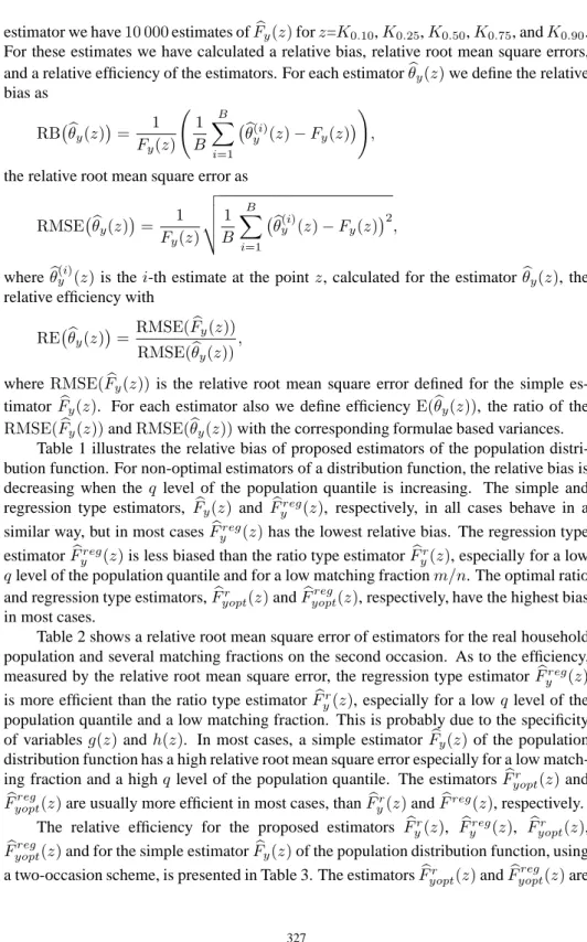
estimator we have10 000estimates ofFby(z)forz=K0.10,K0.25,K0.50,K0.75, andK0.90. For these estimates we have calculated a relative bias, relative root mean square errors, and a relative efficiency of the estimators. For each estimatorθby(z)we define the relative bias as RB θby(z)= 1 Fy(z) 1 B B X i=1 b θ(i) y (z)−Fy(z) ! , the relative root mean square error as
RMSE θby(z)= 1 Fy(z) v u u t1 B B X i=1 b θ(yi)(z)−Fy(z) 2 ,
wherebθ(yi)(z)is thei-th estimate at the pointz, calculated for the estimatorθby(z), the
relative efficiency with
RE θby(z)= RMSE(Fby(z)) RMSE(θby(z)),
whereRMSE(Fby(z))is the relative root mean square error defined for the simple
es-timator Fby(z). For each estimator also we define efficiencyE(bθy(z)), the ratio of the
RMSE(Fby(z))andRMSE(θby(z))with the corresponding formulae based variances.
Table 1 illustrates the relative bias of proposed estimators of the population distri-bution function. For non-optimal estimators of a distridistri-bution function, the relative bias is decreasing when the q level of the population quantile is increasing. The simple and regression type estimators, Fby(z)and Fbreg
y (z), respectively, in all cases behave in a
similar way, but in most casesFbreg
y (z)has the lowest relative bias. The regression type
estimatorFbreg
y (z)is less biased than the ratio type estimatorFbyr(z), especially for a low
qlevel of the population quantile and for a low matching fractionm/n. The optimal ratio and regression type estimators,Fbr
yopt(z)andFb reg
yopt(z), respectively, have the highest bias
in most cases.
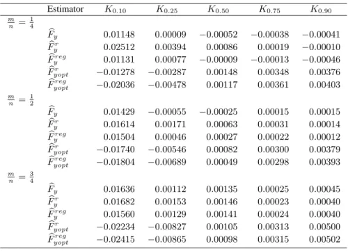
Table 2 shows a relative root mean square error of estimators for the real household population and several matching fractions on the second occasion. As to the efficiency, measured by the relative root mean square error, the regression type estimatorFbreg
y (z)
is more efficient than the ratio type estimatorFbr
y(z), especially for a lowqlevel of the
population quantile and a low matching fraction. This is probably due to the specificity of variablesg(z)andh(z). In most cases, a simple estimator Fby(z)of the population distribution function has a high relative root mean square error especially for a low match-ing fraction and a highqlevel of the population quantile. The estimatorsFbyopt(r z)and
b
Fyoptreg(z)are usually more efficient in most cases, thanFbyr(z)andFbreg(z), respectively.
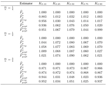
The relative efficiency for the proposed estimators Fbr
y(z), Fbyreg(z), Fbyoptr (z),
b
Fyoptreg(z)and for the simple estimatorFby(z)of the population distribution function, using
a two-occasion scheme, is presented in Table 3. The estimatorsFbr
yopt(z)andFb reg yopt(z)are
Table 1. Relative bias (RB) of estimators Estimator K0.10 K0.25 K0.50 K0.75 K0.90 m n = 1 4 b Fy 0.01148 0.00009 −0.00052 −0.00038 −0.00041 b Fyr 0.02512 0.00394 0.00086 0.00019 −0.00010 b Fyreg 0.01131 0.00077 −0.00009 −0.00013 −0.00046 b Fr yopt −0.01278 −0.00287 0.00148 0.00348 0.00376 b Fyoptreg −0.02036 −0.00478 0.00117 0.00361 0.00403 m n = 1 2 b Fy 0.01429 −0.00055 −0.00025 0.00015 0.00015 b Fr y 0.01614 0.00171 0.00063 0.00031 0.00014 b Freg y 0.01504 0.00046 0.00027 0.00022 0.00012 b Fr yopt −0.01740 −0.00546 0.00082 0.00300 0.00379 b Fyoptreg −0.01804 −0.00689 0.00049 0.00298 0.00393 m n = 3 4 b Fy 0.01636 0.00112 0.00135 0.00025 0.00045 b Fr y 0.01682 0.00153 0.00146 0.00023 0.00040 b Freg y 0.01560 0.00129 0.00141 0.00024 0.00040 b Fr yopt −0.02234 −0.00827 0.00105 0.00313 0.00500 b Fyoptreg −0.02415 −0.00865 0.00098 0.00315 0.00502
Table 2. Relative root mean square error (RMSE) of estimators
Estimator K0.10 K0.25 K0.50 K0.75 K0.90 m n = 1 4 b Fy 0.2066 0.1206 0.0688 0.0397 0.0233 b Fr y 0.2340 0.1192 0.0667 0.0393 0.0233 b Freg y 0.2160 0.1171 0.0659 0.0392 0.0299 b Fr yopt 0.2207 0.1136 0.0639 0.0378 0.0299 b Freg yopt 0.2173 0.1131 0.0637 0.0381 0.0233 m n = 1 2 b Fy 0.2083 0.1195 0.0693 0.0401 0.0299 b Fr y 0.1996 0.1115 0.0642 0.0376 0.0214 b Freg y 0.1969 0.1110 0.0640 0.0375 0.0214 b Fr yopt 0.2065 0.1119 0.0638 0.0378 0.0223 b Freg yopt 0.2040 0.1113 0.0636 0.0378 0.0224 m n = 3 4 b Fy 0.2069 0.1194 0.0687 0.0394 0.0228 b Fyr 0.2377 0.1371 0.0787 0.0455 0.0264 b Freg y 0.2368 0.1370 0.0786 0.0454 0.0263 b Fr yopt 0.2192 0.1159 0.0655 0.0385 0.0244 b Fyoptreg 0.2175 0.1155 0.0654 0.0385 0.0244
Table 3. Relative efficiency (RE) of estimators Estimator K0.10 K0.25 K0.50 K0.75 K0.90 m n = 1 4 b Fy 1.000 1.000 1.000 1.000 1.000 b Fr y 0.883 1.012 1.032 1.012 1.003 b Freg y 0.956 1.030 1.043 1.014 1.017 b Fr yopt 0.936 1.062 1.076 1.050 1.020 b Fyoptreg 0.951 1.067 1.079 1.044 0.999 m n = 1 2 b Fy 1.000 1.000 1.000 1.000 1.000 b Fr y 1.044 1.072 1.080 1.067 1.070 b Freg y 1.058 1.077 1.083 1.069 1.070 b Fr yopt 1.009 1.068 1.087 1.060 1.027 b Fyoptreg 1.021 1.074 1.090 1.062 1.021 m n = 3 4 b Fy 1.000 1.000 1.000 1.000 1.000 b Fyr 0.871 0.871 0.873 0.867 0.866 b Freg y 0.874 0.872 0.874 0.868 0.867 b Fr yopt 0.944 1.031 1.048 1.023 0.936 b Fyoptreg 0.952 1.034 1.051 1.025 0.937
Table 4. Efficiency (E) of estimators
Estimator K0.10 K0.25 K0.50 K0.75 K0.90 m n = 1 4 b Fy 1.000 1.000 1.000 1.000 1.000 b Fr y 0.781 1.004 1.075 1.017 1.002 b Freg y 0.995 1.074 1.113 1.043 1.039 b Fr yopt 1.133 1.163 1.195 1.171 1.219 b Fyoptreg 1.187 1.196 1.213 1.183 1.237 m n = 1 2 b Fy 1.000 1.000 1.000 1.000 1.000 b Fr y 1.092 1.148 1.170 1.145 1.139 b Fyreg 1.126 1.163 1.179 1.151 1.150 b Fyoptr 1.141 1.180 1.204 1.177 1.206 b Fyoptreg 1.183 1.200 1.216 1.185 1.221 m n = 3 4 b Fy 1.000 1.000 1.000 1.000 1.000 b Fr y 0.755 0.761 0.764 0.761 0.760 b Freg y 0.758 0.762 0.765 0.762 0.761 b Fr yopt 1.119 1.121 1.129 1.117 1.152 b Fyoptreg 1.135 1.128 1.134 1.121 1.159
as usual more efficient thanFbr
y(z)and Fbyreg(z), respectively, in most cases. Optimal
estimators mostly have a higher bias shown before. That is a reason why sometimes the efficiency is decreasing, compared with other estimators. The relative efficiency of a simple estimator is higher for the lowestqlevel of the population quantile with a lowest and highest matching fraction. The relative efficiency of the optimal distribution function estimators at the median are highest with any sampling fractions.
The efficiency, ratio of the RMSE with the corresponding formulae based vari-ancesVar(d Fbr
y(z)),dVar(Fbyreg(z)),Var(d Fbyopt(r z)),Var(d Fb reg
yopt(z))andVar(d Fby(z))of the population distribution function, using a two-occasion scheme, is presented in Table 4. Efficiency of proposed optimal estimators using ratio ofRMSEwith the corresponding formulae based variance is grows up comparable with relative efficiency. Average esti-mates of the variances of the proposed optimal ratio and regression estimators are smaller than the empirical variances. The Taylor series expansion of the ratio and regression estimators are used for the expressions of approximate variances. If higher order terms of Taylor expansion would be taken into expression of the approximate variances of these estimators, one can expect to improve the accuracy of the approximation of the variances.
4
Conclusions
We have proposed composite regression and ratio type estimators for a distribution func-tion, as well as optimal estimators, in the sense of minimizing the variance for a two-occasion sampling scheme with a simple random sampling design on each two-occasion. Simulation has been studied on the real population of Lithuanian households of Statistics Lithuania. The simulation results show that the proposed composite estimators using auxiliary information can be used for improving the accuracy of distribution function estimates. The efficiency of the estimators proposed depends on the matching fraction and on the level of quantiles for two-occasion sampling.
References
1. V. Chadyˇsas, Estimation of confidence intervals for quantiles in a finite population, Math.
Model. Anal., 13(2), pp. 195–202, 2008.
2. C. E. S¨arndal, B. Swensson, J. Wretman, Model Assisted Survey Sampling, Springer-Verlag, New York, 1992.
3. R. L. Chambers, R. Dunstan, Estimating distribution functions from survey data, Biometrika, 73, pp. 597–604, 1986.
4. A. H. Dorfman, P. Hall, A comparison of design-based and model-based estimators of the finite population distribution function, Aust. J. Stat., 35, pp. 29–41, 1993.
5. J. N. K. Rao, J. G. Kovar, H. J. Mantel, On estimating distribution functions and quantiles from survey data using auxiliary information, Biometrika, 77, pp. 365–375, 1990.
6. M. Rueda, S. Martinez, H. Martinez, A. Arcos, Estimation of the distribution function with calibration methods, J. Stat. Plan. Infer., 137, pp. 435–448, 2007.
7. P. L. D. N. Silva, C J. Skinner, Estimating distribution functions with auxiliary information using poststratification, Journal of Official Statistics, 11, pp. 277–294, 1995.
8. W. G. Cochran, Sampling Techniques, 3rd ed., Wiley, New York, 1977.
9. G. Kulldorff, Some problems of optimum allocation for sampling on two occasions, Rev. Inst.
Int. Stat., 31(1), pp. 24–57, 1963.
10. H. D. Patterson, Sampling on successive occasions with partial replacement of units, J. Roy.
Stat. Soc. B Met., 12, pp. 241–255, 1950.
11. M. Rueda, J. F. Munoz, S. Gonzales, A. Arcos, Estimating quantiles under sampling on two occasions with arbitrary sample designs, Comput. Stat. Data An., 51, pp. 6956–6613, 2007.