Some Algorithms and Paradigms for Big Data

(1)

Some Algorithms and Paradigms for Big Data

by

Yan Shuo Tan

A dissertation submitted in partial fulfillment of the requirements for the degree of

Doctor of Philosophy (Mathematics)

in the University of Michigan 2018

Doctoral Committee:

Professor Anna Gilbert, Co-Chair

Professor Roman Vershynin, Co-Chair, University of Califor-nia, Irvine

Professor Jinho Baik

Assistant Professor Laura Balzano Professor Alexander Barvinok

(2)

Yan Shuo Tan [email protected] ORCID iD: 0000-0002-6670-9181

(3)

To my parents Chin Kong and Seok Lee, to my sister Yan An, and to Tiffany.

(4)

A C K N O W L E D G E M E N T S

There are many people without whom this dissertation would have been impossible. First, I would like to thank my family in Singapore for their love and support, and for their understanding as four years of absence turned into nine, and as nine now turn into something longer and more indefinite.

I cannot be grateful enough to my adviser Roman Vershynin for his pa-tience and guidance, especially in the early days when I was still strug-gling to find my feet.

I am also grateful to the various faculty, at Michigan and elsewhere, who took the time to offer me knowledge, wisdom, and also kindness. There are too many to name individually, but I would like to especially thank Laura Balzano, Anna Gilbert, Paul Kessenich, and Mahdi Soltanolkotabi. Also, how can I forget my friends and colleagues who have made gradu-ate school such a fun, enlightening, and energetic experience.

Lastly, I would like to thank Tiffany for constantly motivating me to be my best self, for sharing in my sorrow and joy, and for giving me my home away from home.

(5)

PREFACE

From self-driving cars to facial recognition to AlphaGo, the suc-cesses of big data have imprinted it upon the population imagination as a wellspring of technological wonder. Much less obvious to the public, but equally as important from an academic perspective, is the fact that big data has led to a growing synergy amongst the fields of statistics, computer science, and mathematics. In particular, many ideas from both pure and applied mathematics have proved useful in developing and understanding data analysis algorithms and algo-rithmic frameworks. This dissertation is entirely in this spirit. It has given me great joy to draw wield tools from high-dimensional probability, stochastic processes, convex geometry, and even some algebra to chisel out a modest niche in the growing edifice of math-ematical data science.

(6)

LIST OF FIGURES

3.1 Geometry ofWx∗,z . . . 28

3.2 Orientation ofx∗,z, andPzwhena ∈Wx∗,z and whena /∈Wx∗,z. H+andH−

denote respectively the hyperplanes defined by the equations hy,ai = b and

hy,ai = −b. H0 denotes the hyperplane defined by the equation hy,ai = 0. The left diagram demonstrates the situation whena∈Wx∗,z, thereby justifying

(3.8). The right diagram demonstrates the situation whena /∈ Wx∗,z, thereby

justifying (3.11). . . 29

(10)

ABSTRACT

The reality of big data poses both opportunities and challenges to modern re-searchers. Its key features – large sample sizes, high-dimensional feature spaces, and structural complexity – enforce new paradigms upon the creation of effective yet algorithmic efficient data analysis algorithms. In this dissertation, we illus-trate a few paradigms through the analysis of three new algorithms. The first two algorithms consider the problem of phase retrieval, in which we seek to recover a signal from random rank-one quadratic measurements. We first show that an adap-tation of the randomized Kaczmarz method provably exhibits linear convergence so long as our sample size is linear in the signal dimension. Next, we show that the standard SDP relaxation of sparse PCA yields an algorithm that does signal recovery for sparse, model-misspecified phase retrieval with a sample complexity that scales according to the square of the sparsity parameter. Finally, our third algorithm addresses the problem of Non-Gaussian Component Analysis, in which we are trying to identify the non-Gaussian marginals of a high-dimensional distri-bution. We prove that our algorithm exhibits polynomial time convergence with polynomial sample complexity.

(11)

CHAPTER 1

Introduction

1.1 Big Data

We live in the age of big data. As early as 2013, Cukier and Mayer-Schoenberger offered the following striking description for the size of our digital universe [30].

In the third century bc, the Library of Alexandria was believed to house the sum of human knowledge. Today, there is enough information in the world to give every person alive 320 times as much of it as historians think was stored in Alexandria’s entire collection – an estimated 1,200 exabytes’ worth. If all this information were placed on CDs and they were stacked up, the CDs would form five separate piles that would all reach to the moon.

Since then, the sheer quantity of data that we possess has only gotten more ridiculous. Indeed, the digital universe continues to grow at an exponential rate, and is widely projected to double in size once every three years for the foreseeable future. This dizzying trend has captured the popular imagination, and many books have been written investigating its origins and consequences for society. It is not the place of this dissertation to add to this literature. Instead, we offer here a brief sketch of what other people have already said.

The first question to ask is: Where does all of this data comes from? At least some of it is the digitification of information that was previously stored in print or other analog media. Think, for instance, of Google’s project to scan and render machine-readable all of the world’s books. Similar to this is the migration of existing modes of communication and record-keeping to electronic forms – where written correspondence once took place through letters, they now occur via email. Both of these trends have resulted from the power, convenience and accessibility of personal computers, and, more recently, the grow-ing ubiquity of all manner of digital devices. Indeed, accordgrow-ing to Statista, it is projected that more than 36 percent of the world’s population will own a smartphone in 2018 [101].

(12)

Yet, as “smart” devices increasingly penetrate our lives and integrate themselves into our lifestyles, their effect has not merely been to render old forms of data digital, but more consequentially, to createnew kindsof data where there were none before. Take for instance the growing proportion of financial transactions that now take place using credit cards or other electronic payment methods. This allows transactions to be methodically recorded, allowing companies to create electronic profiles of their customers in order to pursue targeted marketing. The burgeoning use of social networks is another example. Again in this case, previously unrecorded information – a person’s social contacts, and her interactions with them – are recorded and “datafied”. Indeed, it seems that almost everyday, new types of data are being created and lending themselves to novel applications. An example from [30] is illustrative.

Appreciating people’s posteriors is the art and science of Shigeomi Koshimizu, a professor at the Advanced Institute of Industrial Technology in Tokyo. Few would think that the way a person sits constitutes information, but it can. When a person is seated, the contours of the body, its posture, and its weight distribu-tion can all be quantified and tabulated. Koshimizu and his team of engineers convert backsides into data by measuring the pressure they exert at 360 differ-ent points with sensors placed in a car seat and by indexing each point on a scale of zero to 256. The result is a digital code that is unique to each individ-ual. In a trial, the system was able to distinguish among a handful of people with 98 percent accuracy. . . . Koshimizu’s plan is to adapt the technology as an anti-theft system for cars.

This explosion of data has presented enormous opportunities for researchers. From a statistical point of view, big data means more covariates or more samples or both, leading to better predictions when fitting traditional statistical models such as linear and logistic regression. Meanwhile, in computer science, a decades-long paradigm shift in artificial intelligence has reached maturity: instead of concocting algorithms directly for comput-ers to perform certain tasks, more success can be attained by letting computcomput-ers “learn” the algorithms themselves through applying learning algorithms to massive amounts of data. Here, the proliferation of data has been married with rapid advances in computing power to make data- and computation-intensive algorithms like deep learning feasible. The stunning success of deep learning has reverberated around academia as well as society as large. Amongst other things, it has enabled self-driving cars, facial recognition, automatic language translation, and AI for Go and other strategy games that can beat the very best human players.

(13)

1.2 A new mathematics of data

While the most visible success of big data has been its technological applications, it has also fertilized much mathematical research. First of all, the diversity of forms of data that we collect behooves us to study new statistical models that model different types of data better. Fitting these models then require new algorithms and strategies. The variety of ways in which data is collected and stored also lends itself to different algorithmic set-ups. For example, there has been much recent work on algorithms that work under the assumption that data is streaming, or that it is distributed across a number of different servers.

In addition, the sheer size of data has posed many interesting theoretical questions. De-spite advances in computational power and resources available on ever smaller computers, there is sometimes more data than can be handled by traditional algorithms within a rea-sonable time frame. As such, there is a need for algorithms that have running times that are linear or even sublinear in their input parameters. In particular, this accounts for the heavy use of gradient descent and stochastic gradient descent in machine learning, and there is now a renewed emphasis on studying first order methods in optimization.

Another way to get around the computational bottleneck is by pre-processing the data to make it more tractable. Two of the most common methods of doing so are (1) data segmentation through clustering and (2) dimension reduction to reduce the number of co-variates. Both of these areas continue to be rich topics of research. Furthermore, now that data is often no longer the only scarce resource, it is useful and important to investigate the trade off between the statistical and computational resources required to achieve a given performance criterion for a given inferential problem.

Thus far, we have discussed questions arising from having data that has both too many samples and too many covariates. In many situations, however, the problem with big data is not simply computational, but also statistical in the sense that we have too many covariates buttoo fewsamples. This is the case, for instance, with genomic data. When trying to pre-dict what genes are prepre-dictive of a higher risk for cancer, a researcher could have, say, tens of thousands of candidate genes, but only a few hundred patients from which DNA samples were taken. Attempting to find the genes naively using linear regression is impossible. The problem, however, becomes feasible when we assert that the signal is sparsein the sense that only a few genes are predictive for cancer. Using such prior knowledge allows one to break sample complexity barriers, and there has been much progress in this direction over the last decade using`1penalty techniques.

Researchers studying theoretical problems inspired by big data are scattered across many different departments. However, there is a growing sense in the community that

(14)

the most rapid progress will come from combining expertise from statistics, computer sci-ence, and other mathematical domains. There is even a place for pure mathematics. Dis-tributional assumptions and the stochastic nature of many big data algorithms mean that randomness is a central feature of the theoretical landscape, leading to heavy use of proba-bilistic tools. Indeed, scalar and matrix concentration inequalities coming from the field of high-dimensional probability are central to the analysis of many algorithms [113].

The usefulness of pure mathematics to big data is not limited to the field of probabil-ity. Theorems from convex geometry are central to analyzing sparse subspace clustering [98, 99]; Grothendieck’s inequality from functional analysis yields sharp guarantees for a community detection algorithm [49]; concepts from Riemannian geometry and dynamic systems shed new light on accelerated optimization methods as well as optimization in non-convex settings [123,71]; algebraic geometry can be used to prove results for learning Gaussian Mixture Models and for filling in missing data [9,83]; tensor decomposition has emerged as a leading strategy for learning latent variable models [3]. These examples are just a slice of the growing synergy between pure mathematics and data science.

My own research, as presented in this dissertation, has been in this spirit. One of the algorithms we shall analyze was inspired by the theory of Fourier Analysis, while another is analyzed using stochastic process theory, and is partially inspired by the theory of Brownian Motion.

1.3 What this dissertation is about

In the last section, we saw how the field of mathematical data science has been developing in an exciting manner. It is again not the place of this dissertation to be a textbook, or even a survey of this emerging field. Instead, we will focus on a few new algorithms, each of which tackles a data science problem in a way that is representative of some broad paradigms for modern mathematical data science. In this section, we will serve a few small appetizers from each of these topics.

1.3.1 Phase retrieval and first order optimization methods

The first problem that we consider is phase retrieval. Mathematically, phase retrieval is the problem of solving systems of rank-1 quadratic equations in_Rn_or

Cn: |hai,xi|2 =b2i, i= 1,2, . . . , N.

(15)

whereai ∈ Rn (orCn) are known sampling vectors,bi > 0 are observed measurements,

andx ∈ _Rn _(or

Cn) is the decision variable. This problem is well motivated by practical

concerns coming from optical imaging and has been a topic of study from at least the early 1980s [43,96].

Early algorithms used in practice were based on alternating minimization, and hence had few theoretical guarantees. The first provably polynomial time algorithm, PhaseLift, was proposed by Cand`es et al in 2013 [22], and was based on semidefinite program-ming. While this was a theoretical breakthrough, the algorithm is not feasible for high-dimensional data. This is because the computational running time for even state-of-the-art SDP solvers does not scale well with the dimensionnof the underlying vector space. Al-gorithms and their time complexity bounds are problem specific, so it is not possible to give a precise description of the running time required. Nonetheless, popular solvers based on interior point methods all have to perform multiple matrix factorizations at each step, each of which require Ω(n3₎_{basic operations. Considering that even 300 by 300 images} are data points in a 90,000-dimensional space, it is clear that more efficient algorithms are required for data coming from real applications.

To address this issue, there has been a growing body of work on first order methods for phase retrieval applied to the natural objective functions associated with the phase retrieval problem. These algorithms are proved to work despite the non-convexity of these objec-tives, and yield rapid speed-ups over PhaseLift. In Chapter3 of this dissertation, we will discuss and prove a guarantee for a stochastic gradient scheme. We will prove that pro-vided we start with an initial estimatex0 that is within constant distance of the true signal vectorx∗, then for any error tolerance, O(n2/)basic operations are sufficient to obtain

an estimateˆx∗that is within distanceofx∗. This is provided that we are givenN = Ω(n)

independent Gaussian measurements. A valid initial estimatex0 can be provably obtained using a spectral initialization method, but numerical experiments show that the algorithm works from arbitrary initializations.

As mentioned in the previous section, first order methods have come to fore in recent years because of the large number of covariates of modern data. In this new regime, sec-ond order methods like Newton’s method are too expensive, thereby removing many of the traditional tools in the optimization toolkit. Often, stochastic schemes such as subsam-pling can also lead to rapid speed-ups, and in this way, our algorithm for phase retrieval is representative of many successful algorithms for big data.

(16)

1.3.2 Sparsity and

`

1

penalties

Sparsity is a major theme that runs through much of modern data science. This is the case first of all because sparsity is a feature of many modern data sets and data analysis problems. For instance, although we now have thousands or even millions of covariates in regression problems, usually only a tiny fraction of them are predictive of the response variable. In signal processing, we often have sparse signals in high dimensional vector spaces and wish to linearly compress them into a vector space of much smaller dimension. In some set ups, naturally occurring signals that are not themselves sparse, such as natural images, become sparse when we use a carefully chosen basis or dictionary.

In addition, sparsity can be thought of as a statistical resource. By assuming that our regression vector is small, we vastly reduce the search space for the regression problem. This allows us to be able to estimate the regression vector with a number of samples that is much smaller than the number of covariates. For instance, if we know that the regression vector is s-sparse, then it is easy to prove that an exhaustive search over all subsets of s coordinates will allow us to estimate the regression vector accurately, so long as we have Ω(slogn)samples. On the other hand, such an exhaustive search is not computationally feasible, so this alone does not yield a scheme for making use of sparsity.

Fortunately, there is actually such a computationally feasible scheme. The idea is to relax the sparsity constraint, which is combinatorial, to an `1-norm constraint, which is geometric. Moreover, since `1-constraint is convex, the theory of convex optimization tells us that it can be incorporated into the linear regression problem in a computationally feasible manner. Finally, we need to be sure that this relaxation is tight, i.e. that the solution to the`1-constrained problem remains the solution to the original sparse regression problem. This turns out to be true when our data matrices satisfy the “restricted isometry property”, which holds with high probability for data that satisfy reasonable distributional assumptions, and when the number of samples is again of the order ofΩ(slogn).

This remarkable sequence of ideas was first discovered by Cand`es, Tao and Romberg [23], and applies also to the signal processing setting we mentioned earlier: one can com-press ans-sparse signalsby applying a known random projectionA. The original signal can then be recovered from the compressed vectorx := Asusing the linear programming method described above. Their work helped to found the modern field of compressed sens-ing, which continues to be a highly active today.

It is natural to extend the theoretical framework of sparsity and`1-regularized optimiza-tion to phase retrieval. The phase retrieval model differs from that of linear regression only in the sense that linear measurements are replaced with quadratic measurements. Indeed both models are instances of single index models, the study of which have a rich history in

(17)

statistics. Furthermore, the signal vectors that arise in phase retrieval are often sparse [96]. As such, it is unsurprising that there is already a body of work on the problem of sparse phase retrieval. For a brief overview of the literature, see Chapter4.

1.3.3 Model misspecification in sparse phase retrieval

When trying to model real world data with parametric statistical models, it is also important to account for the possibility that the model might be misspecified, or in other words, that the true distribution does not lie in the parametric family that we have assumed. Whenever this is likely, we need to have algorithms that are robust, i.e. that the estimate produced by our algorithm continue to have good predictive power, however this is quantified.

In the case of linear regression, a common way in which model misspecification hap-pens is that instead of having linear measurements, we receive measurements of the form

bi :=f(hai,x∗i), i= 1,2, . . . , N.

Here,f is an unknown, possibly random, link function. Indeed, real data is never precisely linear. Nonetheless, naive linear regression continues to work well as an algorithm for estimatingx∗(up to norm), and researchers have for some time been usingLassoand other

sparse linear regression algorithms for data in which the response variable is clearly non-linear, as is the case when it is discrete.

Plan and Vershynin were able to justify this practice theoretically in their work on the non-linear Lasso in 2016 [87]. They showed that, assuming that the measurement vectorsai’s are independent Gaussians, then Lasso continues to work with the same sample

complexity guarantee so long as the link functionf satisfies some regularity properties, and such that it is “positively correlated” with a true linear function.

Again, it is natural to extend this framework to the setting of phase retrieval. Here, we are concerned with having measurements that are not precisely quadratic. Note that the earlier analysis for Lasso does not apply to this setting because our unknown link functions should still be close in some sense to the square function, which is easily shown to be “uncorrelated” with linear functions.

In order to overcome this, we propose combining the “lifting” procedure of PhaseLift [22] with the “correlation maximization” algorithm that Plan and Vershynin proposed to solve the problem of 1-bit compressed sensing [85]. It turns out that the resulting algo-rithm is essentially the convex relaxation of sparse PCA proposed some years earlier by d’Aspremont et al. [31]. We are able that our algorithm has sample complexityO(s2_log_n), wheresis again the sparsity parameter. This matches the performances of other algorithms

(18)

that have been proposed for sparse phase retrieval. Nonetheless, it is not information theo-retic optimal, and it is an open question whether the optimal rate can be achieved. We will pursue this discussion in much more detail in Chapter4.

1.3.4 Learning with moments

One way to fit a parametric model is to use the method of moments. This method has a long and venerable history, having been first proposed and used by no less than Karl Pearson in 1894. Pearson had a set of data comprising the ratio of forehead to body length for 1000 crabs, and believed the crabs to have come from two different species rather than one. As such, he postulated that the forehead to body length ratio measurements could be modeled by the sum of two Gaussian components, which he then fit by matching the first 6 moments of the model with the empirical moments that he computed from the data [76].

More generally, the method of moments proceeds as follows: we estimate the parameter θto be the value such that the moments of the distribution µθ are “close” to the empirical

moments computed from sample data, which in the basic setting comprises independent copies of a random variable drawn from the true distribution. Here, “closeness’ means different things in different contexts. While Pearson first proposed the method to study distributions on _R, it can also be applied to distributions on _Rn. It is important to note that the moments of multivariate distributions are not scalars but tensors, and this adds an additional layer of complexity.

Recently, the method has been successfully applied to provide polynomial time algo-rithms for learning various latent variable models [54, 3], including topic models, hidden Markov models, and high-dimensional Gaussian mixture models. There are two key ideas that underpin these algorithms. First, the low-order moment tensors of the distributions have low-rank decompositions, i.e. each of them can be written as the sum of a small num-ber of pure tensors). The individual pure tensors summands the yield information about the model parameter vector θ. Second, there is a robust polynomial time method for finding these low-rank decompositions [3].

Another variant of the method of moments also yield a polynomial time algorithm for solving the problem of Independent Component Analysis (ICA). ICA is a semi-parametric model that has applications to blind source separation. In this model, the signal is a random vectors in_Rn _{with independent non-Gaussian entries, and the observations made by the}

observer are of the formx =As, whereAis an unknownnbynmixing matrix. The goal of the problem is to learn the mixing matrixA. The algorithm, introduced by Frieze et al. [44] and further studied by Arora et al. [4] is an iterative algorithm based on local search.

(19)

It exploits the fact that the columns of Aare the local optima for the 4-th order moment tensor, i.e. for the functionf: Sn−1 _→

Rdefined by

f(v) :=_E{hv,xi4}.

In summary, we see that the method of moments is a useful tool for many learning problems.

1.3.5 Dimension reduction through linear projections

The high-dimensional nature of many modern data sets make many otherwise useful data analysis algorithms inefficient, especially those whose running time scales as a high degree polynomial in the dimension of the ambient vector space. On the other hand, theintrinsic dimension of the data is usually a lot smaller than its ambient dimension. For instance, it is often the case the signal in the data is localized to a low-dimensional subspace. In such a situation, one would like to do dimension reduction. We would like to project the data to its “true” subspace, and run our algorithms on the projected data points instead, thereby leading to potentially massive speedups.

There are many methods for dimension reduction in the literature. We will mention two of the most basic here, both of which involve linear projections. Principal Compo-nent Analysis (PCA) involves projecting the data points to a subspace of maximal vari-ance. Practically, one forms the sample covariance matrix of the data, computes its eigen-decomposition, and then projects the data to the subspace spanned by the topk eigenvec-tors, wherekis an algorithmic parameter that is supplied using prior knowledge or through model selection. The motivation for PCA is the assumption that the directions with more variance have more “explanatory value”. This would be true, for example, if the data arises from points lying on a subspace perturbed by a small amount of orthogonal noise.

Random projections have also turned out to be very useful. The celebrated Johnson-Lindestrauss lemma tells us that the pairwise`2 distances betweenN points are preserved under a random projection to a vector space of dimension Ω(logN). In this instance, by random, we mean that the target subspace is drawn uniformly from the relevant Grassman-nian. Indeed, random projections tend to preserve the “structure” of “data” so long as the target space has large enough dimension.

One way to make this precise is in the setting of structured regression. Suppose we are given the prior information that a signal x∗ lies in a compact set K ⊂ Rn. Then x∗ can

be estimated from a random projection Px∗ so long as the target subspace has dimension

(20)

K, and we see that square corresponds to the “statistical dimension” of the set [115]. This has connections to the “M∗ bound” and related theory in geometric functional analysis.

Apart from preserving information while simultaneously allowing us to work in a lower-dimensional space, random projections are also cheap to compute. This is because tall matrices with independent Gaussian entries are approximate isometries whose column spans are drawn uniformly from the Grassmannian. Such matrices are easy to construct us-ing pseudorandom number generators. This fact allows us to have speedups in computus-ing approximate matrix factorizations via random projections, thereby contributing to much of the success of randomized numerical linear algebra [50].

1.3.6 NGCA and reweighted PCA

In the problem of Non-Gaussian Component Analysis (NGCA), we assume that we have data points in a low dimensional subspace E that are perturbed by orthogonal Gaussian noise. The goal is to estimate this structured subspaceE. If the noise is a lot smaller than the variance of the points withinE, we can solve this problem using PCA. If this is either unknown or not the case, then new assumptions and ideas are needed.

A reasonable assumption to make is that the data points have non-Gaussian marginals in the directions that lie in E. In this case, we can use moment information to determine the non-Gaussian directions, thereby finding E. Indeed, this is what Vempala and Xiao proposed in 2011 [112]. Their idea was to adapt the local search algorithm proposed for solving ICA that we have discussed in a previous section [44]. Recall that this algorithm is able to recover the columns of the mixing matrixAas the local optima of the fourth moment tensor. In the NGCA case, we no longer assume that there areindependentnon-Gaussian directions, so a much more delicate analysis is required. Furthermore, we no longer assume that the non-Gaussian marginals differ from a Gaussian in the fourth moment. As such, higher moment tensors have to be considered.

Although Vempala and Xiao’s algorithm comes with a polynomial running time and sample complexity guarantee, it is fairly complicated and requires delicate parameter tun-ing. Furthermore, it is rather computationally inefficient. In Chapter6, we will show that NGCA can also be solved by the far easier algorithm of reweighted PCA. To run this al-gorithm, we first place the data points in isotropic position. Next, we attach to each data pointXithe weight exp(−αkXik

2

2), whereαis a parameter that can either be chosen with prior knowledge, or found through the running of the algorithm. We next do PCA on the reweighted sample, and then extract non-Gaussian directions as the eigenvectors to outlier eigenvalues.

(21)

Performing PCA with a reweighted sample has been applied successfully in several other contexts [18,48]. In our case, the reason why it works is because of a new character-ization of multi-dimensional Gaussian distributions: we are able to tell whether a random vector X is a standard Gaussian by inspecting the moments of its norm kXk₂ and those of its dot product with an independent copyhX,X0i. This moment information can be ex-tracted from the reweighted sample covariance matrix, as well as from an auxiliary matrix that has be used in adversarial situations.

We will develop the characterization theorem further in Chapter5. The theory turns out to also be useful for proving several theorems on energy minimization for distributions on the sphere.

1.4 Notes

Many of the results in this dissertation have been the result of joint work with my adviser, Roman Vershynin. Each of the following chapters is based on work that is available as a preprint or published paper. See [107,108,105,106].

(22)

CHAPTER 2

High-Dimensional Probability

2.1 What is high-dimensional probability?

High-dimensional probability is the study of random objects defined over_Rnor_Cn, where nis a large but fixed number. Such objects include vectors, matrices, tensors, and graphs. Despite its fundamental importance today, the reader may notice that there aren’t many text-books on high-dimensional probability, the reason being that the field is still very young, both in content and in name. Traditionally, probability theorists were interested in asymp-totic results such as Central Limit Laws or in stochastic process theory. Many of the ideas, techniques and theorems in what we now call high-dimensional probability were instead developed to answer questions in geometric functional analysis, and later, non-asymptotic random matrix theory.

In recent years, researchers studying algorithms either possessing internal randomiza-tion or handling data with distriburandomiza-tional assumprandomiza-tions naturally found themselves faced with questions about high-dimensional random objects. Sometimes, these questions could be answered with simple concentration inequalities such as Chernoff’s inequality, but often, more sophisticated results are called for. As such, results from high-dimensional probabil-ity have begun to garner more attention, and in a synergistic manner, the field has begun to take on more independent research interest, emerging out of the shadow of geometric functional analysis into a more cohesive whole.

In this chapter, we collate some results from high-dimensional probability that will be used in the rest of this dissertation. These are collated from [70], [110], [113], [74], as well as several other sources that will be mentioned where appropriate.

(23)

2.2 ψ

α

random variables

Definition 2.2.1(Orlicz norms). Letψ: _R+ → R+ be a convex, increasing function with ψ(0) = 0. Define theOrlicz normof a random variableX with respect toψas

kXk_α := inf{λ >0 : _E{ψ(|X|/λ)} ≤1}.

Equipped with this norm, the space of random variables with finite norm forms a Banach space, called anOrlicz space.

We are especially interested in the Orcliz spaces corresponding toψαforα >0. These

are defined as follows. Whenα≥1, we setψα(x) := exp(xα)−1. When0< α≤1, this

function is no longer convex, so we convexify it by fiat, settingψα(x) := exp(xα)−1for

x ≥ x(α)large enough, and takingψα to be linear on[0, x(α)]. If some random variable

Xhas a finiteψαnormkXk_ψ_α, we say that it is aψαrandom variable.

Readers may already be familiar with ψ2 and ψ1 Orcliz spaces. These correspond to subgaussianandsubexponentialrandom variables respectively (see [113] for more details). For these two classes of random variables, we have the well-known Hoeffding’s and Bern-stein’s inequalities.

Proposition 2.2.2(Hoeffding’s inequality). LetX1, . . . , Xmbe independent, centered,

sub-gaussian random variables. Then for everyt≥0, we have

P ( m X i=1 Xi ) ≤2 exp − ct 2 Pm i=1kXik 2 ψ2 ! ,

wherec >0is an absolute constant.

Proposition 2.2.3(Bernstein’s inequality). LetX1, . . . , Xmbe independent, centered,

subex-ponential random variables. Then for everyt≥0, we have

P ( m X i=1 Xi ) ≤2 exp −cmin ( t2 Pm i=1kXik2ψ1 , t maxikXikψ1 )! ,

wherec >0is an absolute constant.

In subsequent chapters, however, it will be useful for us to consider Orlicz spaces in full generality. This is because we will need to work withψ1/2random variables, for which many of the standard concentration inequalities do not hold. Nonetheless, we still have the following.

(24)

Proposition 2.2.4(Characterization ofψ1/2RVs). LetXbe a real-valued random variable. Then the following properties are equivalent. The parametersCi > 0appearing in these

properties differ from each other by at most an absolute contant factor.

1. The tails ofX satisfy

P{|X| ≥t} ≤2 exp

−pt/C1

.

2. The moments ofXsatisfy

kXk_p = (_E|X|p)1/p≤C2p2.

3. Theψ1/2 norm ofXsatisfies

kXk_ψ

1/2 ≤C3.

Proof. Same as in the case ofψ1 andψ2. See [113]. We have the following further properties.

Proposition 2.2.5(Products, Lemma 8.5 in [74]). Let X andY beψα random variables

for someα >0. ThenXY is aψα/2 random variable withψα/2 norm satisfying

kXYk_ψ

α/2 ≤CαkXkψαkYkψα.

Here,Cαis an absolute constant depending only onα.

Proposition 2.2.6(Centering). LetX be aψαrandom variable for someα >0. Then kX−_EXk_ψ

α ≤2kXkψα.

Proof. We havekX−_EXk_ψ

α ≤ kXkψα+kEXkψα. Now check the definition of the norm

to verify thatk_EXk_ψ

α ≤ kXkψα.

Proposition 2.2.7(Sums, Theorem 6.21 in [70]). Let0< α≤1, and letX1, . . . , Xm be a

sequence of independent, centeredψα random variables. Then

m X i=1 Xi ψα ≤Cα E m X i=1 Xi + max 1≤i≤m|Xi| ψα ! .

(25)

Proposition 2.2.8(Maxima, Lemma 2.2.2 in [110]). Let0 < α ≤ 1, and letX1, . . . , Xm

be independent, centeredψαrandom variables. Then

max 1≤i≤m|Xi| ψα ≤Cαψα−1(m) max 1≤i≤mkXikψα.

Here,Cαis an absolute constant depending only onα.

Proposition 2.2.9 (Bernstein-type inequality for ψ1/2 RVs). Let X1, . . . , Xm be an

in-dependent, centered ψ1/2 random variables. There is an absolute contant C such that Sm := √1_m

Pm

i=1Xi is aψ1/2 random variable withψ1/2 norm satisfying

kSmkψ1/2 ≤C₁max_≤_i_≤_mkXikψ1/2.

In particular, ifmax1≤i≤mkXikψ1/2 is bounded above by a constant, for everyt ≥ 0, we

have

P{|Sm| ≥t} ≤2 exp(−

p t/C).

Proof. This follows more or less immediately from the last two propositions. First, notice that E m X i=1 Xi ≤  E m X i=1 Xi 2  1/2 ≤C√m max 1≤i≤mkXikψ1/2

Here, the first inequality is an application of Jensen’s inequality, and the second uses the moment bound in Proposition2.2.4. Next, we computeψ_α−1(m) = (log(m+ 1))2, and use Proposition2.2.8, we get max 1≤i≤m|Xi| ψα ≤C(logm)2 max 1≤i≤mkXikψα.

Finally, plug these two bounds into the inequality given by Proposition2.2.7, and note thatlog(m+ 1)/√m ≤ 5. This completes the proof of the first statement. The tail bound follows from Proposition2.2.4.

2.3 Subgaussian random vectors and random matrices

We say that a random vector X in_Rn _is _subgaussian_{if all one-dimensional marginals of}

X are subgaussian. Furthermore, if all these marginals have subgaussian norm bounded by a constantK, we abuse notation slightly and say thatX has subgaussian norm kXk_ψ2

(26)

Theorem 2.3.1(Concentration of norm for general sub-Gaussian vectors). LetXbe a sub-Gaussian random vector in _Rn, with kXk_ψ2 ≤ K. There is a universal constant C such that for each positive integerr >0, the moments ofkXk₂ andhX,X0isatisfy

(_E{kXkr₂})1/r ≤CK(√n+√r) (2.1)

(_E{|hX,X0i|r})1/2r ≤CK(√n+√r). (2.2) Proof. The second bound follows from the first, since by Cauchy-Schwarz,

(_E{|hX,X0i|r})1/2r ≤(_E{kXkr₂kX0kr₂})1/2r= (_E{kXkr₂})1/r

To prove (2.1), pick a 1₂-netN onSn−1_{. A volumetric argument shows that one may pick}

N to have size no more than5n_{(see [114]). We then have} kXk₂ = sup

v∈Sn−1

hX,vi ≤2 sup

v∈N

hX,vi.

By definition, there is a universal constantcsuch that for any fixed unit vector v ∈ Sd−1_,

P{hX,vi> t} ≤2 exp

−ct2 K2

. Taking a union bound over the net thus gives

P{kXk2 >2t} ≤2 exp nlog 5− ct 2 K2 . (2.3)

Next, we integrate out the tail bound (2.3) to obtain bounds for the moments. Observe that if ₂ct_K22 ≥ nlog 5, we havenlog 5−

ct2

K2 ≤ −

ct2

2K2. This condition on t is equivalent to

t≥CK√n, so we have P{kXk2 >2t} ≤    1 t < CK√n 2 exp−ct2 K2 t≥CK√n (2.4)

For any positive integerr, we integrate this bound to get

E{kXkr2}= Z ∞ 0 rtr−1_P{kXk> t}dt ≤ Z CK √ n 0 rtr−1dt+ Z ∞ CK√n 2rtr−1exp −ct 2 K2 dt ≤CrKrnr/2+CrKrr Z ∞ 0 tr/2−1e−tdt.

(27)

The integral in the last line is the gamma function, so in short, we have shown that

E{kXkr2} ≤C

r

Kr(nr/2+ Γ(r/2 + 1)). (2.5) Takingr-th roots of both sides and using H¨older, together with the fact thatΓ(x)1/x _. x, gives (2.1).

Lemma 2.3.2(Covariance estimation for sub-Gaussian random vectors). LetX be a cen-tered sub-Gaussian random vector in _Rn with covariance matrix Σ and sub-Gaussian norm satisfying kXk_ψ2 ≤ K for some K ≥ 1. Let ΣˆN = _N1 PN_i₌₁XiXTi denote the

sample covariance matrix from N independent samples. Then there is an absolute con-stant C such that for any 0 < , δ < 1, we have _Pn

ˆ ΣN −Σ > o ≤ δ so long as N ≥CK2_(n_{+ log(1/δ))}−2_.

Proof. This is essentially Theorem 5.39 in [114].

Lemma 2.3.3 (Moments of spherical marginals). Let θ be uniformly distributed on the sphereSn−1. Then for any unit vectorv∈Sn−1 and any positive integerk, we have

E{hθ,vi2k}=

1·3· · ·(2k−1)

n·(n+ 2)· · ·(n+ 2k−2) (2.6)

Proof. There are several ways to prove this identity. We shall prove this by computing Gaussian integrals. Letg andg_n denote standard Gaussians in 1 dimension and n dimen-sions respectively. Then using the radial symmetry ofg, we have

E{g2k}=E{hgn,vi 2k_} =_E{hkg_nk₂θ,vi2k}=_E{kg_nk2₂k}_E{hθ,vi2k}. Rearranging gives E{hθ,vi2k}= E{g 2k_} E{kgnk 2k 2 } . We then compute E{kgnk 2k 2 }= ωn (2πn)n/2 Z ∞ 0 r2krn−1e−r2/2dr, (2.7) whereωnis the volume of the sphereSn−1. It is well known that

ωn=

2πn/2 Γ(n/2),

(28)

while we also have

Z ∞ 0

r2krn−1e−r2/2dr = 2n/2+k−1Γ(n/2 +k). Substituting these back into (2.7) gives

E{kgnk

2k

2 }= 2

kΓ(n/2 +k)

Γ(n/2) =n·(n+ 2)· · ·(n+ 2k−2). (2.8) This yields the denominator in (2.6). A similar calculation forE{g2k}yields the numerator.

2.4 Chaining

Many concentration inequalities for random vectors and random matrices make use of net arguments. For example, consider Lemma2.3.2for bounding the operator norm of a ran-dom matrix. To prove this, one makes use of the fact that the operator norm of annby n matrixAis defined as

kAk= sup

v∈Sn−1

kAvk. (2.9)

The net argument is to approximate the supremum over the sphere by a maximum over an -net, that is, a collection of pointsN for which every other point on the sphere is-close to a point inN. The error is then controlled using continuity properties of the`2norm. In this case, as in many others, such an argument produces optimal results. However, this is not always the case.

To see why, it is insightful to view (2.9) as saying that kAk is the supremum of a random process (Xv) indexed by v over the index set Sn−1. This supremum is bounded

by considering the process increments Xv − Xu at a scale of kv−uk ≈ , where is

the parameter of the net that we are using. In the matrix case, the choice of was not too important, but on many occasions it is. Worse still is the situation where, because of the non-uniformly of process increments, there is not a single choice ofthat works best, . In this case, it is helpful to try to consider all scales simultaneously. One way to address this is using the idea of generic chaining, which was first invented by Talagrand [70,104]. We shall use a variant of his approach which is appropriate for our purposes. This approach was developed by Dirksen in [38].

Let (T, d) be a metric space. A sequence T = (Tk)k∈Z+ of subsets of T is called

(29)

functionalof(T, d)to be γα(T, d) := inf T sup_t_∈_T ∞ X k=0 2k/αd(t, Tk). (2.10)

Letd1 andd2be two metrics onT. We say that a process(Yt)hasmixed tail increments

with respect to(d1, d2)if there are constantscandCsuch that for alls, t ∈T, we have the bound

P(|Ys−Yt| ≥c( √

ud2(s, t) +ud1(s, t)))≤Ce−u. (2.11) Remark2.4.1. In [38], processes with mixed tail increments are defined as above but with the further restriction thatc = 1 andC = 2. This is not necessary for the result that we need (Lemma 2.4.2) to hold. The indeterminacy of cand C gets absorbed into the final constant in the bound.

Lemma 2.4.2 (Mixed tail processes, Theorem 5 in [38]). If(Yt)t∈T has mixed tail

incre-ments, then there is a constantC such that for anyu≥1, with probability at least1−e−u_,

sup

t∈T

|Yt−Yt0| ≤C(γ2(T, d2) +γ1(T, d1) +

√

udiam(T, d2) +udiam(T, d1)).

At first glance, theγ2andγ1quantities seem mysterious and intractable. We will show however, that they can be bounded by more familiar quantities that are easily computable in our situation. First, given a setT with metricd, we define the covering number ofT at scaleu to bethe smallest number of radius u balls needed to cover T. We denote this quantity byN(T, d, u). Interchanging the supremum and the sum in (2.10), and then doing a few usual tricks yields the famous Dudley inequality.

Lemma 2.4.3(Dudley’s inequality). For eachα >0, there is an absolute constantCαfor

which for any metric space(T, d), one has

γα(T, d)≤Cα

Z ∞ 0

(logN(T, d, u))1/αdu. (2.12)

2.5 Growth functions and VC dimension

Unlike most of the topics that we have discussed thus far, growth functions and VC dimen-sion emerged not out of geometric functional analysis, but instead as part of an attempt to proof uniform limit laws in statistics. The theory first started with Vapnik and Cher-vonenkis’s foundational paper [111], and has since grown into an indispensable tool for

(30)

theoretical machine learning, and in particular PAC theory. We state here some definitions and standard results that will be required in3.5. We refer the interested reader to [91] for a more in-depth exposition on these topics.

Let X be a set and C be a family of subsets ofX. For a given setC ∈ C, we slightly abuse notation and identify it with its indicator function 1C: X → {0,1}. The growth

functionΠC:N→RofC is defined via

ΠC(m) := max

x1,...,xm∈X

|{(C(x1), C(x2), . . . , C(xm)) : C ∈ C}|.

Meanwhile, the VC dimension of C is defined to be the largest integer m for which ΠC(m) = 2m. These two concepts are fundamental to statistical learning theory. The key

connection between them is given by the Sauer-Shelah lemma.

Lemma 2.5.1(Sauer-Shelah, Corollary 3.3 in [91]). LetC be a collection of subsets of VC dimensiond. Then for allm≥d, have

ΠC(m)≤

em d

d .

The reason why we are interested in the growth function of a family of subsets C is because we have the following guarantee for the uniform convergence for the empirical measures of sets belonging toC.

Proposition 2.5.2(Uniform deviation, Theorem 2 in [111]). LetC be a family of subsets of a setX. Letµbe a probability measure onX, and letµˆm := _m1

Pm

i=1δXi be the empirical

measure obtained frommindependent copies of a random variableX with distributionµ. For everyusuch thatm ≥2/u2_{, the following deviation inequality holds:}

P(sup C∈C

|µˆm(C)−σ(C)| ≥u)≤4ΠC(2m) exp(−mu2/16). (2.13)

We now state and prove two simple claims.

Claim 2.5.3. LetC be the collection of all hemispheres inSn−1_{. Then the VC dimension of}

C is bounded from above byn+ 1.

Proof. It is a standard fact from statistical learning theory [91] that the VC dimension of half-spaces in_Rnisn+ 1. SinceSn−1is a subset of_Rn, the claim follows by the definition of VC dimension.

(31)

Claim 2.5.4. LetC andDbe two collections of functions from a setX to{0,1}. Using4

to denote symmetric difference, we define

C4D :={C4D|C ∈ C, D ∈ D}. (2.14) Then the growth function ΠC4D of C4D satisfies ΠC4D(m) ≤ ΠC(m) ·ΠD(m) for all

m∈_Z+.

Proof. Fixm, and pointsx1, . . . , xm ∈ X. Then every possible configuration(f(x1), f(x2), . . . , f(xm))arising from somef ∈ C4D is the point-wise symmetric difference

(f(x1), f(x2), . . . , f(xm)) = (C(x1), C(x2), . . . , C(xm))4(D(x1), D(x2), . . . , D(xm))

of configurations arising from some C ∈ C and D ∈ D. By the definition of growth functions, there are at mostΠC(m)·ΠD(m)pairs of these configurations, from which the

bound follows.

Remark2.5.5. There is an extensive literature on how to bound the VC dimension of con-cept classes that arise from finite intersections or unions of those from a known collection of concept classes, each of which has bounded VC dimension. We won’t require this much sophistication here, and refer the reader to [17] for more details.

(32)

CHAPTER 3

Phase Retrieval and the Randomized Kaczmarz

Method

3.1 Introduction

The mathematical phase retrieval problem is that of solving a system of quadratic equations

|hai,zi2|=b2i, i= 1,2, . . . , m (3.1)

whereai ∈ Rn (orCn) are known sampling vectors,bi > 0 are observed measurements,

and z ∈ _Rn _(or

Cn) is the decision variable. The solution to the problem, x∗, is called

the signal vector. It is customary to use terminology from signal processing in the phase retrieval, since the mathematical problem is inspired by practical applications to do with signal recovery.

One such application is Coded Diffraction Imaging (CDI). In this procedure, a small two-dimensional object is illuminated by a coherent wave, and its far field diffraction in-tensity pattern is observed. The inin-tensity function so derived corresponds roughly to the squared magnitude of the 2D Fourier transform of the object’s transmittance function. The problem of recovering the transmittance function then fits into the framework of our math-ematical model (3.1). x∗ is now the discretized transmittance function, while the ai’s are

2D DFT vectors. Generally, the high frequency spectrum of light waves makes it impossi-ble for optical detection devices to measure their phase. Having to recovery a signal from the amplitudes of its Fourier transform is thus a central feature of optical imaging. Phase retrieval also arises naturally in many other settings in science and engineering, including electron microscopy, crystallography, and astronomy.

In line with the development of optical imaging, researchers have proposed and studied algorithms to address phase retrieval since at least the 1970s. The first algorithms, such as those proposed by Gerchberg-Saxton and Fienup were based on alternating projections

(33)

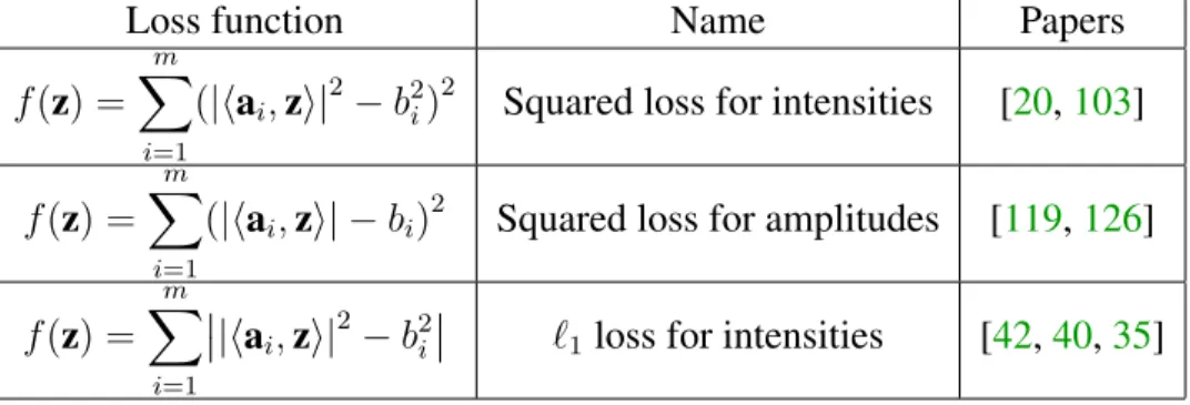
Loss function Name Papers f(z) = m X i=1 (|hai,zi| 2

−b2_i)2 Squared loss for intensities [20,103] f(z) =

m

X

i=1

(|hai,zi| −bi)2 Squared loss for amplitudes [119,126]

f(z) = m X i=1 |ha_i,zi| 2

−b2_i `₁loss for intensities [42,40,35] Table 3.1: Non-convex loss functions for phase retrieval

[43, 96]. These were shown to exhibit empirical convergence to a global minimum in the noise-free oversampled setting, but were not robust to noise, and had few theoretical guarantees.

Over the last half a decade, there has been great interest in constructing and analyzing algorithms with provable guarantees given certain classes of sampling vector sets. One line of research involves “lifting” the quadratic system to a linear system, which is then solved using convex relaxation (PhaseLift) [22]. A second method is to formulate and solve a linear program in the natural parameter space using an anchor vector (PhaseMax) [47, 6, 52]. Although both of these methods can be proved to have near optimal sample efficiency, the most empirically successful approach has been to directly optimize various naturally-formulated non-convex loss functions, the most notable of which are displayed in Table3.1.

These loss functions enjoy nice properties which make them amenable to various op-timization schemes [103, 42]. Those with provable guarantees include the prox-linear method of [40], and various gradient descent methods [20, 26, 119, 126, 35]. Some of these methods also involve adaptive measurement pruning to enhance performance.

In 2015, Wei [121] proposed adapting a family of randomized Kaczmarz methods for solving the phase retrieval problem. He was able to show using numerical experiments that these methods perform comparably with state-of-the-art Wirtinger flow (gradient descent) methods when the sampling vectors are real or complex Gaussian, or when they follow the coded diffraction pattern (CDP) model [20]. He also showed that randomized Kaczmarz methods outperform Wirtinger flow when the sampling vectors are the concatenation of a few unitary bases. Unfortunately, [121] was not able to provide adequate theoretical justification for the convergence of these methods (see Theorem 2.6 in [121]).

In this chapter, we attempt to bridge this gap by showing that the basic randomized Kaczmarz scheme used in conjunction with truncated spectral initialization achieves lin-ear convergence to the solution with high probability, whenever the sampling vectors are

(34)

drawn uniformly from the sphere1 Sn−1 _{and the number of measurements}_m_{is larger than} a constant times the dimensionn.

It is also interesting to note that the basic randomized Kaczmarz scheme is exactly stochastic gradient descent for the Amplitude Flow objective, which suggests that other gradient descent schemes can also be accelerated using stochasticity.

3.1.1 Randomized Kaczmarz for solving linear systems

The Kaczmarz method is a fast iterative method for solving systems of overdetermined lin-ear equations that works by iteratively satisfying one equation at a time. In 2009, Strohmer and Vershynin [102] were able to give a provable guarantee on its rate of convergence, pro-vided that the equation to be satisfied at each step is selected using a prescribed randomized scheme.

Suppose our system to be solved is given by

Ax=b, (3.2)

whereAis anmbynmatrix. Denoting the rows ofAbyaT

1, . . . ,aTm, we can write (3.2) as

the system of linear equations

hai,xi=bi, i= 1, . . . , m.

The solution set of each equation is a hyperplane. The randomized Kaczmarz method is a simple iterative algorithm in which we project the running approximation onto the hyperplane of a randomly chosen equation. More formally, at each step k we randomly choose an index r(k)from [m] such that the probability that r(k) = i is proportional to

kaik2₂, and update the running approximation as follows:

xk :=xk−1+ br(k)− har(k),xk−1i kar(k)k 2 2 ar(k).

Strohmer and Vershynin [102] were able to prove the following theorem:

Theorem 3.1.1(Linear convergence for linear systems). Letκ(A) =kAk_F/σmin(A). Then for any initialization x0 to the equation (3.2), the estimates given to us by randomized Kaczmarz satisfy

Ekxk−x∗k2₂ ≤ 1−κ(A)−2

k

kx0−x∗k2₂.

1_{This is essentially equivalent to being real Gaussian because of the concentration of norm phenomenon}

(35)

Note that ifAhas bounded condition number, thenκ(A)√n.

3.1.2 Randomized Kaczmarz for phase retrieval

In the phase retrieval problem (3.1), each equation

|hai,x∗i|=bi

defines two hyperplanes, one corresponding to each of ±x. A natural adaptation of the randomized Kaczmarz update for this situation is then to project the running approximation to thecloser hyperplane. We restrict to the case where each measurement vectoraihas unit

norm, so that in equations, this is given by

xk :=xk−1+ηkar(k), (3.3) where

ηk=sign(har(k),xk−1i)br(k)− har(k),xk−1i.

In order to obtain a convergence guarantee for this algorithm, we need to choosex0 so that it is close enough to the signal vector x∗. This is unlike the case for linear systems

where we could start with an arbitrary initial estimatex0 ∈Rn, but the requirement is par for the course for phase retrieval algorithms. Unsurprisingly, there is a rich literature on how to obtain such estimates [22,26,126,119]. The best methods are able to obtain a good initial estimate usingO(n)samples.

3.1.3 Main results

The main result of this chapter guarantees the linear convergence of the randomized Kacz-marz algorithm for phase retrieval for random measurements ai that are drawn

indepen-dently and uniformly from the unit sphere.

Theorem 3.1.2 (Convergence guarantee for algorithm). Fix > 0, 0 < δ1 ≤ 1/2, and 0< δ, δ2 ≤1. There are absolute constantsC, c >0such that if

m≥C(nlog(m/n) + log(1/δ)),

then with probability at least1−δ, m sampling vectors selected uniformly and indepen-dently from the unit sphereSn−1_{form a set such that the following holds: Let}_x_∈

Rnbe a

signal vector and letx0 be an initial estimate satisfyingkx0−x∗k₂ ≤c

√

(36)

any >0, if

K ≥2(log(1/) + log(2/δ2))n,

then theK-th step randomized Kaczmarz estimatexK satisfieskxK−x∗k2₂ ≤kx0−x∗k2₂

with probability at least1−δ1−δ2.

Comparing this result with Theorem3.1.1, we observe two key differences. First, there are now two sources of randomness: one is in the creation of the measurementsai, and the

other is in the selection of the equation at every iteration of the algorithm. The theorem gives a guarantee that holds with high probability over both sources of randomness. Theo-rem3.1.2also requires an initial estimatex0. This is not hard to obtain. Indeed, using the truncated spectral initializationmethod of [26], we may obtain such an estimate with high probability givenm_&n. For more details, see Proposition3.7.1.

The proof of this theorem is more nontrivial than the Strohmer-Vershynin analysis of randomized Kaczmarz algorithm for linear systems [102]. We break down the argument in smaller steps, each of which may be of independent interest to researchers in this field.

First, we generalize the Kaczmarz update formula (3.3) and define what it means to take a randomized Kaczmarz step with respect to any probability measure on the sphereSn−1: we choose a measurement vector at each step according to this measure. Using a simple geometric argument, we then provide a bound for the expected decrement in distance to the solution set in a single step, where the quality of the bound is given in terms of the properties of the measure we are using for the Kaczmarz update (Lemma3.2.1).

Performing the generalized Kaczmarz update with respect to the uniform measure on the sphere corresponds to running the algorithm with unlimited measurements. We utilize the symmetry of the uniform measure to compute an explicit formula for the bound on the stepwise expected decrement in distance. This decrement is geometric whenever we make the update from a point making an angle of less thanπ/8with the true solution, so we obtain linear convergence conditioned on no iterates escaping from the “basin of linear convergence”. We are able to bound the probability of this bad event using a supermartin-gale inequality (Theorem3.3.1).

Next, we abstract out the property of the uniform measure that allows us to obtain lo-cal linear convergence. We lo-call this property the anti-concentration on wedges property, calling it ACW for short. Using this convenient definition, we can easily generalize our previous proofs for the uniform measure to show that all ACW measures give rise to ran-domized Kaczmarz update schemes with local linear convergence (Theorem3.4.3).

The usual Kaczmarz update corresponds running the generalized Kaczmarz update with respect toµA:= _m1

P

(37)

and independently from the sphere, then µA satisfies the ACW condition with high

prob-ability, so long as m _& n (Theorem3.5.7). The proof of this fact uses VC theory and a chaining argument, together with metric entropy estimates.

Finally, we are able to put everything together to prove a guarantee for the full algorithm in Section3.6. In that section, we also discuss the failure probabilitiesδ, δ1 and δ2, and how they can be controlled.

3.1.4 Notes

This chapter is adapted from the paper “Phase Retrieval via Randomized Kaczmarz: The-oretical Guarantees” [107]. During the preparation of that manuscript, we became aware of independent simultaneous work done by Jeong and G¨unt¨urk. They also studied the ran-domized Kaczmarz method adapted to phase retrieval, and obtained almost the same result that we did (see [61] and Theorem 1.1 therein). In order to prove their guarantee, they use a stopping time argument similar to ours, but replace the ACW condition with a stronger condition called admissibility. They prove that measurement systems comprising vectors drawn independently and uniformly from the sphere satisfy this property with high prob-ability, and the main tools they use in their proof are hyperplane tessellations and a net argument together with Lipschitz relaxation of indicator functions.

After submitting the first version of the manuscript, we also became aware of indepen-dent work done by Zhang, Zhou, Liang, and Chi [126]. Their work examines stochastic schemes in more generality (see Section 3 in their paper), and they claim to prove linear convergence for both the randomized Kaczmarz method as well as what they called Incre-mental Reshaped Wirtinger Flow. However, they only prove that the distance to the solution decreases in expectation under a single Kaczmarz update (an analogue of our Lemma3.2.1

specialized to real Gaussian measurements). As we will see in this chapter, this bound cannot be naively iterated.

3.2 Computations for a single step

In this section, we will compute what happens in expectation for a single update step of the randomized Kaczmarz method. It will be convenient to generalize our sampling scheme slightly as follows. When we work with a fixed matrixA, we may view our selection of a random rowar(k)as drawing a random vector according to the measureµA := _m1

Pm

i=1δai.

(38)

µon the sphereSn−1_{, we define the random map}_P₌_P

µon vectorsz ∈Rnby setting

Pz:=z+ηa, (3.4)

where

η=sign(ha,zi)|ha,x∗i| − ha,zi and a∼µ. (3.5)

Note that as before, x∗ is a fixed vector in Rn (think of x∗ as the actual solution of the

phase retrieval problem). We callPµ thegeneralized Kaczmarz projection with respect to

µ. Using this update rule over independent realizations ofP, P1,P2, . . ., together with an initial estimatex0, gives rise to ageneralized randomized Kaczmarz algorithmfor finding x∗: set thek-th step estimate to be

xk:=PkPk−1· · ·P1x0. (3.6)

Fix a vectorz∈_Rn_{that is closer to}_x

∗than to−x∗, i.e. so thathx∗,zi>0, and suppose

that we are trying to findx∗. Examining the formula in (3.5), we see thatPprojectszonto

the right hyperplane (i.e., the one passing through x∗ instead of the one passing through

−x∗) if and only ifha,ziandha,x∗ihave the same sign. In other words, this occurs if and

only if the random vectoradoesnotfall into the region of the sphere defined by Wx∗,z :={v∈S

n−1_|_sign(_h_v,_x

∗i)6=sign(hv,zi)}. (3.7)

This is the region lying between the two hemispheres with normal vectorsx∗ and z. We

call such a region aspherical wedge, since in three dimensions it has the shape depicted in Figure3.1.

Figure 3.1: Geometry ofWx∗,z

Whena∈/ Wx∗,z, we can use the Pythagorean theorem to write

(39)

−x∗ x∗ z Pz H+ H− H0 −x∗ x∗ z Pz H+ H− H0 |ha,2xi| |ha,z−x∗i|

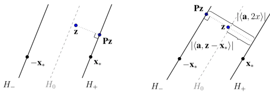
Figure 3.2: Orientation of x∗, z, andPz when a ∈ Wx∗,z and when a /∈ Wx∗,z. H+ and

H− denote respectively the hyperplanes defined by the equationshy,ai = b andhy,ai =

−b. H0 denotes the hyperplane defined by the equation hy,ai = 0. The left diagram demonstrates the situation when a ∈ Wx∗,z, thereby justifying (3.8). The right diagram

demonstrates the situation whena /∈Wx∗,z, thereby justifying (3.11).

Rearranging gives

kPz−x∗k2₂ =kz−x∗k2₂(1− h˜z,ai2), (3.9)

where˜z= (z−x∗)/kz−x∗k₂.

In the complement of this event, we get

Pz=z+ha,(−x∗)−zia=z− ha,z−x∗i+ha,−2x∗i,

and using orthogonality,

kPz−x∗k2₂ =kz−x∗k2₂− ha,z−x∗i2 +ha,2x∗i2. (3.10)

Sincezgets projected to the hyperplane containing−x∗, it may move further away from

x∗. However, we can bound how far away it can move. Because ha,x∗ihas the opposite

sign asha,zi, we have

|ha,z+x∗i|<|ha,z−x∗i|,

and so

|ha,2x∗i|=|ha,(z−x∗)−(z+x∗)i|<2|ha,z−x∗i|.

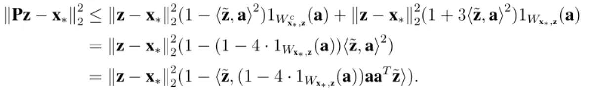
Substituting this into (3.10), we get the bound

kPz−x∗k2₂ ≤ kz−x∗k2₂ + 3ha,z−x∗i2 =kz−x∗k2₂(1 + 3h˜z,ai2), (3.11)

(40)

We can combine (3.9) and (3.11) into a single inequality by writing kPz−x∗k2₂ ≤ kz−x∗k2₂(1− h˜z,ai2)1Wc x∗,z(a) +kz−x∗k 2 2(1 + 3h˜z,ai 2 )1Wx∗,z(a) =kz−x∗k2₂(1−(1−4·1Wx∗,z(a))h˜z,ai 2 ) =kz−x∗k2₂(1− h˜z,(1−4·1Wx∗,z(a))aa T_˜_z_i_).

Taking expectations, we can remove the role that˜zplays by bounding this as follows.

E[kz−x∗k2₂(1− h˜z,(1−4·1Wx∗,z(a))aa T_˜ zi)] =kz−x∗k2₂(1− h˜z,E[(1−4·1Wx∗,z(a))aa T_]˜_z_i₎ ≤ kz−x∗k2₂ 1−λmin(EaaT −4EaaT1Wx∗,z(a)) . We may thus summarize what we have obtained in the following lemma.

Lemma 3.2.1(Expected decrement). Fix vectorsx∗,z ∈ Rn, a probability measureµon

Sn−1_{, and let}_P ₌_P

µ,Wx∗,zbe defined as in(3.4)and(3.7)respectively. Then

EkPz−x∗k2₂ ≤

1−λmin(EaaT −4EaaT1Wx∗,z(a))

kz−x∗k2₂.

Let us next compute what happens forµ=σ, the uniform measure on the sphere. It is easy to see that_EaaT ₌ 1

nIn, so it remains to computeEaa T₁

Wx∗,z(a). To do this, we make

a convenient choice of coordinates: Letθ be the angle betweenzandx∗. We assume that

both points lie in the plane spanned by e1 ande2, the first two basis vectors, and that the angle betweenzandx∗ is bisected bye1, as illustrated in Figure3.3.

Figure 3.3: Choice of coordinates

For convenience, denoteM :=_EaaT1Wx∗,z(a). LetQdenote the orthogonal projection

operator onto the span of e1 and e2. Then Q(Wx∗,z) is the union of two sectors of angle

Some Algorithms and Paradigms for Big Data