CIRJE Discussion Papers can be downloaded without charge from: http://www.e.u-tokyo.ac.jp/cirje/research/03research02dp.html
Discussion Papers are a series of manuscripts in their draft form. They are not intended for circulation or distribution except as indicated by the author. For that reason Discussion Papers may
CIRJE-F-625
Probability Distribution and Option Pricing for
Drawdown in a Stochastic Volatility Environment
Kyo Yamamoto
Graduate School of Economics, University of Tokyo Seisho Sato
Institute of Statistical Mathematics Akihiko Takahashi
University of Tokyo June 2009
Probability Distribution and Option Pricing for
Drawdown in a Stochastic Volatility Environment
Kyo Yamamoto
∗,Seisho Sato
†, and Akihiko Takahashi
∗First vesion: 28 November, 2008
This version: 4 May, 2009
Forthcoming in
International Journal of Theoretical and Applied Finance
Abstract
This paper studies the probability distribution and option pricing for drawdown in a stochastic volatility environment. Their analytical approx-imation formulas are derived by the application of a singular perturbation method (Fouqueet al. [7]). The mathematical validity of the approxima-tion is also proven. Then, numerical examples show that the instantaneous correlation between the asset value and the volatility state crucially affects the probability distribution and option prices for drawdown.
1
Introduction
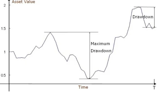
In asset management business, drawdown related risk measures, such as maxi-mum drawdown, are considered very important for the risk investigation of mu-tual or hedge funds. Drawdown related risk measures are defined in a dynamic setting. Let {St}0≤t≤T be a stochastic process that represents the net asset
value of a fund. Drawdown of{St}0≤t≤T at timetis defined byDt=Mt−St,
where Mt = max0≤u≤tSu. In other words, drawdown is the lost wealth of
investors from the record high level. Maximum drawdown is its historical max-imum. (See Fig. 1.) Drawdown related risk measures fit hedge fund managers as well as investors. Most hedge funds set high water mark provision in the fee structures. It means that hedge fund managers receive a fixed rate performance fee of exceeding the high water mark, or record high level. In other words, they cannot get performance fee during suffering drawdown. Therefore, the risk for fund managers is exactly drawdown.
∗The University of Tokyo
Methods of portfolio optimization with controlling drawdown have been de-veloped so far. Grossman and Zhou [11] proposed an portfolio optimization of a risk-free asset and a risky asset under drawdown constraints in the Black-Scholes economy. It solved the optimization problem by dynamic programming. Cvitanic and Karatzas [3] extended it to multi-risky asset and more general settings, and solved the optimization problem by martingale method. Chekhlov
et al. [2] introduced a risk measure conditional drawdown (CDD) and proposed a portfolio optimization method with controlling CDD. Hakamada et al. [12] and Krokhmalet al. [15] applied the method to portfolio construction of hedge funds.
Properties of (maximum) drawdowns have also been studied. Magdon-Ismail
et al. [18] and Magdon-Ismail and Atiya [16] researched the probability distri-bution of maximum drawdowns for Brownian motion and geometric Brown-ian motion, respectively. Belentepe [1] examined the probability distribution drawdown for geometric Brownian motion, and then considered how portfo-lio diversification reduced the expected drawdown. Vecer [22] studied relation between directional trade and maximum drawdown (and drawup), and Vecer [23] considered pricing and hedging contingent claims on maximum drawdown. These two research papers implemented the analysis by Monte Carlo simulation under the assumption that the underlying asset followed geometric Brownian motion. Pospisil and Vecer [20] analyzed it by a PDE method under the same assumption.
This article studies the probability distribution and option pricing for draw-down in a stochastic volatility environment by an analytical approach. The option for drawdown can be a powerful risk management tool. Their analytical approximation formulas are derived by applying a singular perturbation method (Fouqueet al. [7]). Fouqueet al. [7] argues the method for option pricing in detail. The accuracy of the approximation is examined in Yamamoto and Taka-hashi [25]. In this paper, it is shown that the first order stochastic volatility term is linearly related to the instantaneous correlation between asset value and volatility state. The mathematical validity of the approximation for European option is shown by Fouqueet al. [8]. This article proves that the validity is also held for the analysis of drawdown. Our numerical examples clarified that the correlation affects the probability distribution and option prices for draw-down. If asset value and volatility state are positively correlated, the expected drawdown is higher than those for uncorrelated case or Black-Scholes economy, and the standard deviation of drawdown is lower than those cases. Due to the effect of the correlation on the probability distribution, the option prices for drawdowns are also affected by the correlation.
The organization of the paper is as follows. The next section studies the probability distribution and pricing options of drawdowns in the Black-Scholes economy. In section 3, they are considered in a stochastic volatility environment. Section 4 presents numerical examples. Section 5 concludes. In appendix A, the singular perturbation method for our problem is explained. Appendix B proves the convergence result of the approximation.
2
Drawdown in the Black-Scholes Economy
First, probability distribution and option pricing for drawdown are considered in the Black-Scholes economy. Let (Ω,F,P,{Ft}0≤t≤T <∞) be a complete
probabil-ity space with a filtration satisfying the usual conditions. There are a risk-free asset with a constant risk-free rate r, and a risky asset. In (Ω,F,P,{Ft}) ,
it is assumed that the risky asset price {St} follows the stochastic differential
equation (SDE)
dSt=µStdt+σStdWt1,
where{W1
t}is a standard Brownian motion, andµandσis a constant. Defining
Mt= max0≤u≤tSu, the drawdown from time 0 totis given by
Dt=Mt−St.
In other words, drawdown is the lost wealth of investors from the record high level. For the purpose of convenience, we calculate the joint probability of
Figure 1: Drawdown and Maximum Drawdown
(ST, MT) through their logarithm. LetXt= logStandZt= logMt. Then,
dXt= ( µ−σ 2 2 ) dt+σdWt1, X0=x0,
andZt= max0≤u≤tXu We first calculate the simultaneous probability density
function of (XT, ZT). ForZt< b, let
Then, by Feynman-Kac’s theorem,PBS(t, x;a, b) is the solution of the boundary value problem LBSPBS(t, x;a, b) = 0, PBS(t, b;a, b) = 0, PBS(T, x;z, b) = 1{x≤a} where LBS= ∂ ∂t + ( µ−σ 2 2 ) ∂ ∂x+ σ2 2 ∂2 ∂x2.
By method of images (See, for example, Wilmottet al. [24].), PBS is obtained
by PBS(t, x;a, b) =N(d1(T−t, x))−exp{(2µ/σ2−1)(b−x)}N(d2(T−t, x)), (1) where d1(s, x) = a−x−(µ−σ2/2)s σ√s , d2(s, x) = a+x−2b−(µ−σ2/2)s σ√s .
Differentiating (1) with respect to a and b, we get the simultaneous density function of (XT, ZT). Then, for any function g of (ST, MT), E[g(ST, MT)] is
evaluated by E[g(ST, MT)] = ∫ ∞ x0 ∫ b −∞ g(ea, eb)∂ 2P0 BS ∂a∂b (0, x;a, b)dadb.
For example, the distribution functionF(c) = P(DT ≤c) and nth moment of
drawdown is obtained by setting g(ST, MT) = 1{MT−ST≤a} and g(ST, MT) =
(MT −ST)n, respectively.
Next, proceed to the calculation of option prices for drawdown. In the economy, the risk neutral measure is defined by
P∗(A) =E[exp(−θW1
T−θ
2T /2)1
A] for A∈ F,
whereθ= µ−σr. By Maruyama-Girsanov’s theorem, when{Wt1∗}is defined by
Wt1∗=W
1
t +θt,
it is a standard Brownian motion underP∗. Let
PBS∗ (t, x;a, b) =P∗(XT ≤a, ZT ≤b |Xt=x, Zt< b).
SinceXtfollows the SDE
dXt= ( r−σ 2 2 ) dt+σdWt1∗,
the previous argument under the risk neutral measure shows thatPBS∗ (t, x;a, b) is given by
PBS∗ (t, x;a, b) =N(d∗1(T−t, x))−exp{(2r/σ2−1)(b−x)}N(d∗2(T−t, x)), (2) where d∗1(s, x) =a−x−(r−σ 2/2)s σ√s , d ∗ 2(s, x) = a+x−2b−(r−σ2/2)s σ√s .
Therefore, the call option prices for drawdown with strikeKand maturityT at time 0 is given by C(0, x) =E∗[e−rT(MT−ST−K)+] =e−rT ∫ ∞ x0 ∫ b −∞ (eb−ea−K)+ ∂2P∗ BS ∂a∂b (0, x;a, b)dadb.
If we have assetS and this option, the drawdown ofS exceedingK is covered by the option. Therefore, this option can be a powerful risk management tool against drawdowns.
3
Drawdown in a Stochastic Volatility
Environ-ment
Next, the argument of previous section is extended to a stochastic volatility circumstance. In (Ω,F,P,{Ft}) , it is assumed that the risky asset price {St}
follows the SDE
dSt=µStdt+σtStdWt1,
where{Wt1}is a standard Brownian motion, andµis a constant. The volatility
σt is the stochastic process expressed as follows by using Ornstein-Uhlenbeck
(OU) process{Yt}. σt=f(Yt), dYt= 1 ϵ(m−Yt)dt+ν √ 2 ϵdW 2 t, Y0=y0,
where f is a positive increasing function, and {Wt2} is a standard Brownian motion that have instantaneous correlationρ∈(−1,1) with{Wt1},
d〈W1, W2〉=ρdt.
It is assumed thatf and 1
f are bounded: there are constantsl1andl2such that
0< l1≤f(y)≤l2<∞ for any y∈R.
Explanations for the parameters are given shortly. mis a constant, andϵandν
are positive constants. In accordance with [7], the fast mean-reverting stochastic volatility is supposed, and consequentlyϵis a positive small number. As shown
in Fouqueet al. [7], {Yt} has the normal invariant distribution N(m, ν2).
Fi-nally,ρis a constant that expresses the instantaneous correlation between{St}
and{Yt}.
We calculate the simultaneous probability density function of (XT, ZT). For
a < b, let
PSV(t, x, y;a, b) =P(XT ≤a, ZT ≤b |Xt=x, Yt=y, Zt< b). (3)
Then, by Feynman-Kac’s theorem,PSV(t, x, y;a, b) is the solution of the
bound-ary value problem
Lϵ SVPSV(t, x, y;a, b) = 0, PSV(t, b, y;a, b) = 0, PSV(T, x, y;a, b) = 1{x≤a}, where Lϵ SV = 1 ϵL0+ 1 √ ϵL1+L2, L0=ν2 ∂ 2 ∂y2 + (m−y) ∂ ∂y, L1= √ 2νρf(y)∂x∂y∂2 , L2= ∂t∂ + ( µ−12f(y)2)∂ ∂x+ 1 2f(y) 2 ∂2 ∂x2.
The value ofPSV is approximated up to the order of
√
ϵby singular perturbation method. From Appendix A, the approximation up to the first order stochastic volatility correction is given by
PSV(t, x, y;a, b)≈PSV0 (t, x;a, b) +
√
ϵPSV1 (t, x;a, b), (4) where P0
SV(t, x;a, b) is equal to the value of PBS with constant volatility
pa-rameter ¯σ, which is defined by ¯σ=√〈f2〉, where〈·〉represents the expectation
under the invariant distribution ofY: N(m, ν2). P1
SV(t, x;a, b) is the first order
stochastic volatility correction term, which is of order√ϵ. The first two terms of the expansion do not depend ony. According to A.2, PSV0 is the solution of the boundary value problem
〈L2〉PSV0 (t, x;a, b) = 0 in 0< x < b and t < T, P0 SV(t, b;a, b) = 0, PSV0 (T, x;a, b) = 1{x≤a}, where〈L2〉=∂t∂ + ( µ−σ¯22 ) ∂ ∂x+ ¯ σ2 2 ∂2 ∂x2. By method of images,P 0 SV is given by PSV0 (t, x;a, b) =N(d1(T−t, x))−exp{(2µ/σ¯2−1)(b−x)}N(d2(T−t, x)), (5) where d1(s, x) = a−x−(µ−¯σ2/2)s ¯ σ√s , d2(s, x) = a+x−2b−(µ−σ¯2/2)s ¯ σ√s .
As described in A.3, the first order stochastic volatility correction term
PSV1 (t, x;a, b) is the solution of the boundary value problem
〈L2〉PSV1 (t, x;a, b) =V ( ∂3 ∂x3 − ∂2 ∂x2 ) P0 SV(t, x;a, b) in 0< x < b and t < T, P1 SV(t, b;a, b) = 0, PSV1 (T, x;a, b) = 0. (6) V is a constant defined by V = √ρν 2〈f φ ′〉, (7)
whereφ′ is a function ofy defined in (16). Defining ˆ PSV(t, x;a, b) = 1 VP 1 SV(t, x;a, b) + (T−t) ( ∂3 ∂x3− ∂2 ∂x2 ) PSV0 (t, x;a, b),
the inhomogeneous boundary value problem (6) is transformed into the following homogeneous problem; 〈L2〉PˆSV(t, x;a, b) = 0 in 0< x < b and t < T, ˆ PSV(t, b;a, b) = (T−t) ( ∂3 ∂x3− ∂2 ∂x2 ) P0 SV(t, b;a, b), ˆ PSV(T, x;a, b) = 0. ˆ
PSV is obtained by numerical integration as follows. The probabilistic
rep-resentation of ˆPSV is ˆ PSV(t, x;a, b) =E [ (T−τ) ( ∂3 ∂x3 − ∂2 ∂x2 ) PSV0 (τ, b;a, b)1{τ≤T}¯¯¯Xt0=x ] , whereX0
t is the stochastic process that satisfies SDE
dXt0= ( µ−σ¯ 2 2 ) dt+ ¯σdWt1,
andτ is the first time aftertthatX0hitsb. Changing a variable and using the distribution of the first hitting time of Brownian motion (see e.g. Karatzas and Shreve [14], Chapter 2, Proposition 8.5),
ˆ PSV(t, x;a, b) = ∫ T t (T−s) ( ∂3 ∂x3 − ∂2 ∂x2 ) PSV0 (s, b;a, b)h(s;x, b)ds, (8) where h(s;x, b) = b−x ¯ σ√2π(s−t)3exp [ −{b−x−(µ−σ¯2/2)(s−t)}2 2¯σ2(s−t) ] .
If the integration in (8) is evaluated numerically, PSV1 (t, x;a, b) is obtained by PSV1 (t, x;a, b) =V { ˆ PSV(t, x;a, b)−(T −t) ( ∂3 ∂x3 − ∂2 ∂x2 ) PSV0 (t, x;a, b) } .
Consequently, the approximation ofPSV is obtained by
PSV(t, x;a, b)≈PSV0 (t, x;a, b) +
√
ϵPSV1 (t, x;a, b). (9) The next theorem confirms the validity of the approximation.
Theorem 1 Under the assumption that f and 1
f is bounded, at a fixed point
t < T,x, y∈R,
PSV(t, x, y;a, b) =PSV0 (t, x;a, b) +
√
ϵPSV1 (t, x;a, b) +O(ϵ).
Proof. See Appendix B.
Differentiating this with respect to aand b, the approximate simultaneous probability density function of (XT, ZT) is obtained. Stochastic volatility affects
the simultaneous probability distribution of (XT, ZT) throughV defined in (7).
V depends on ρ, which represents the instantaneous correlation between the asset value and the volatility, andν, which scales the volatility of volatility. For any functiong of (ST, MT),E[g(ST, MT)] is approximately evaluated by
E[g(ST, MT)] = ∫ ∞ x0 ∫ b −∞ g(ea, eb)∂ 2P0 SV ∂a∂b (0, x;a, b)dadb +√ϵV ∫ ∞ x0 ∫ b −∞ g(ea, eb)∂ 2PˆSV ∂a∂b (0, x;a, b)dadb −√ϵV T ∫ ∞ x0 ∫ b −∞ g(ea, eb) ( ∂5P0 SV ∂x3∂a∂b− ∂4P0 SV ∂x2∂a∂b ) (0, x;a, b)dadb.
The first term is the Black-Scholes part, and the second and third terms are the first order stochastic volatility correction part. Note that the first order correction term is linearly related toV, and therefore linearly related toρ.
Next, proceed to the calculation of option prices for drawdown. While risk-neutral measure is uniquely determined in the Black-Scholes economy, there are infinitely many risk-neutral measures in this economy, because the market is incomplete. The risk-neutral measure depends on the market price of volatility risk. For simplicity, it is assumed that the stochastic process ofSt under
risk-neutral measureP∗is described as follows.
dSt=rStdt+σtStdWt1∗, S0=ex0,
where {W1∗
t } is a standard Brownian motion under P∗. The volatility σt is
the stochastic process expressed as follows by using Ornstein-Uhlenbeck (OU) process{Yt}.
dYt= 1 ϵ(m−Yt)dt+ν √ 2 ϵdW 2∗ t , Y0=y0, where{W2∗
t }is a standard Brownian motion that have instantaneous correlation
ρ∈(−1,1) with {W1∗
t }. Let
PSV∗ (t, x;a, b) =P∗(XT ≤z, ZT ≤b |Xt=x, Zt< b).
The previous argument under the risk neutral measure shows that the approx-imate value ofPSV∗ is obtained by changingµappeared in (9) to r. Then, the approximate prices of call option for drawdown with strikeK and maturityT
at time 0 is given by C(0, x) =E∗[e−rT(MT−ST−K)+] =e−rT ∫ ∞ x0 ∫ b 0 (eb−ea−K)+ ∂2PSV∗ ∂a∂b (0, x;a, b)dadb.
Sure, it can be calculated under other risk-neutral measures. In other words, we can allow for market price of volatility risk as Fouqueet al. [7]. Parameters ¯
σ and √ϵV can be calibrated from the implied volatilities of liquid European call options (see e.g. Fouqueet al. [7]).
4
Numerical Examples
This section presents some numerical examples. First, expectation and standard deviation of drawdown are studied. We setS0= 100, and assign
f(y) =
{
10−10+ey (y <0),
10−10+ 2−e−y (y≥0).
Then, f and 1/f are bounded. The parameter settings are as follows. Since Fouqueet al. [7] found fast mean-reverting volatility, this paper also considers the case;ϵ= 1/200, for example. We setµ= 0.15, m=−1.89, ν = 0.40, and
T = 1/12. Then, ¯σ= 0.2. Since stochastic volatility affects the distribution of drawdown through parameterρ, we consider three patterns: ρ=−0.75, 0, 0.75. As previously mentioned, whenρ= 0, the first order stochastic volatility cor-rection term is 0. Therefore, the statistics for ρ = 0 is equal to those in the Black-Scholes economy withσ= 0.2.
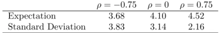
ρ=−0.75 ρ= 0 ρ= 0.75 Expectation 3.68 4.10 4.52 Standard Deviation 3.83 3.14 2.16
Table 1: Expactations and standard deviations of drawdowns
Table 1 exhibits the expectations and standard deviations of drawdowns. Positive instantaneous correlation between the asset and the volatility state
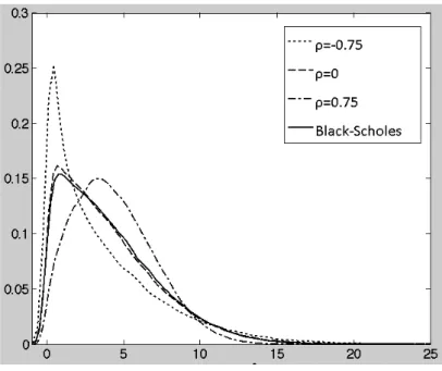
Figure 2: Probability Density of Drawdown
increases expected drawdown, while negative correlation decreases. And the positive correlation decreases standard deviation of drawdown, while negative correlation increases it.
Fig. 2 shows the probability density function estimated by Monte Carlo simulation. This graph enables us to observe the effect of correlations on the probability distribution of drawdown visually. The density functions of draw-downs for the cases of ρ = 0 and Black-Scholes look very similar. From this figure, it is confirmed again that a positive correlation increases expected draw-down, while a negative correlation decreases it.
Next, proceed to numerical studies of options for drawdown. The parameter settings are same as the above analysis, and we set the risk-free rate asr= 0.02. For determination of strike level, expectations and standard deviations under the risk-neutral measure are also calculated. In the analysis, approximation accuracies are also studied.
In order to obtain the estimate value of the options for the two cases, Monte Carlo simulations with antithetic variables method are conducted. The num-ber of the simulation is 1,000,000. Since the volatility of Y is very high, the time step should be very small in order to converge the simulations of Y. Time step is determined in the following way. For the case of f(y) = ey,
the distribution of Y at the terminal date is known analytically. In order to match the distribution of simulations and analytic one, ∆t = 1/100,000 is needed. Therefore, this time step is used in our analysis. Table 2
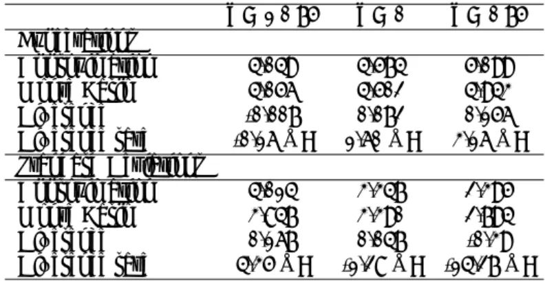
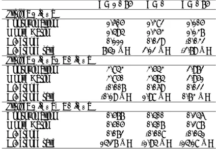
ex-hibits the numerical results. The statistics calculated by the approximation method and Monte Carlo simulations are reported. In addition, we exhibit dif-ference and difference rate between the approximation value and Monte Carlo value, which are given by (Approximate value−M onte Carlo value) and (Approximate value−M onte Carlo vaue)/(M onte Carlo value) respectively. We note that there are other ways than Monte Carlo methods. For example, Pospisil and Vecer [20] applied a PDE method in the analysis of maximum drawdown. ρ=−0.75 ρ= 0 ρ= 0.75 Expectations Approximation 4.049 4.574 5.099 Monte Carlo 4.056 4.502 4.943 Difference -0.007 0.072 0.156 Difference rate -0.16Å? 1.60Å? 3.16Å? Standard Deviations Approximation 4.014 3.347 2.395 Monte Carlo 3.847 3.390 2.794 Difference 0.167 0.047 -0.39 Difference rate 4.35Å? -1.28Å? -14.27Å?
Table 2: Expectations and standard deviations under risk-neutral measure Table 2 shows that the expected drawdowns can be calculated with some accuracy by our approximation method. The relation betweenρ and expected drawdowns is also confirmed by Monte Carlo simulations. As for standard deviations, for the case ofρ= -0.75 and 0.75, the differences result in relatively high compared to those for expectations. However, the relation betweenρand standard deviations can be also found by Monte Carlo simulations.
Next, calculate option prices for drawdown. In practice, strike levels vary among option buyers according to their risk attitudes. Hence, three different strikes are chosen based on the empirical statistics of drawdown. First, the strike is set to the expected drawdownE[DT]. The other two strikes are above
and below 1 standard deviation from expected drawdown. Note that since the statistics are different byρ, strikes vary according toρin this analysis.
Reading across the rows of the table, the option prices decrease inρ. This is because dispersion ofDT decrease inρas shown in Table 2, where dispersion
levels are measured by standard deviation.
Next, the approximation accuracy of our method is discussed. For the case ofρ= 0, the errors of the approximation method are about 2% for all strikes. As forρ= 0.75 andρ=−0.75, the errors for the options with strikesE[DT]−
SD[DT] are relatively small compared to other strikes. Finally, note that the
difference rates for the options with strikesE[DT]−SD[DT] are relatively high
for the case of ρ = 0.75 and ρ = −0.75. This strike corresponds to out-of-the-money (OTM) for the plain vanilla option. Yamamoto and Takahashi [25]
ρ=−0.75 ρ= 0 ρ= 0.75 Strike: E[DT] Approximation 1.605 1.382 1.105 Monte Carlo 1.494 1.353 1.137 Difference 0.111 0.029 -0.032 Difference rate 7.41Å? 2.12Å? -2.79Å? Strike: E[DT]−SD[DT] Approximation 3.843 3.543 2.972 Monte Carlo 3.850 3.474 2.951 Difference -0.007 0.069 0.022 Difference rate -0.19Å? 1.98Å? 0.73Å? Strike: E[DT] +SD[DT] Approximation 0.577 0.400 0.246 Monte Carlo 0.505 0.407 0.287 Difference 0.072 -0.008 -0.041 Difference rate 14.27Å? -1.94Å? -14.18Å?
Table 3: Option prices for drawdown
reported the result that the difference rates of this method for plain vanilla European call OTM options are also relatively high. Our result agrees with that evidence.
5
Conclusion
This article studied the probability distribution and option pricing for drawdown in a stochastic volatility environment. Their analytical approximation formulas were derived by the application of a singular perturbation method (Fouqueet al.
[7]), and it showed that the first order stochastic volatility term is linearly related to the instantaneous correlation between asset value and volatility state. The mathematical validity of the approximation was also shown. Then, numerical examples clarified that the correlation crucially affects the probability distri-bution and option prices for drawdown. If they are positively correlated, the expected drawdown is higher than those for uncorrelated case or Black-Scholes economy, and standard deviation of drawdown is lower than those cases. Due to the effect of the correlation on the probability distribution of drawdown, the option prices for drawdowns are also affected by the correlation.
A
Singular Perturbations
This appendix presents singular perturbation method (Fouqueet al. [7]) for our problem. First, the general framework is described. Then, the Black-Scholes term and the first order stochastic volatility correction term are derived. Further details of this method for option pricing are argued in Fouqueet al. [7].
A.1
Formal Expansion
First, a formal asymptotic expansion is conducted. The economical setting is the same as section 3. Consider the drawdown of the underlying assetS frome time 0 toT. LetPSV(t, x, y;a, b) be defined by (3). By Feynman-Kac’s theorem,
PSV satisfies the following partial differential equation (PDE);
Lϵ SVPSV = 0 in (0, T)×(−∞, b)×R (10) where Lϵ SV = 1 ϵL0+ 1 √ ϵL1+L2, L0=ν2 ∂ 2 ∂y2 + (m−y) ∂ ∂y, L1= √ 2νρf(y) ∂2 ∂x∂y L2= ∂t∂ + ( µ−12f(y)2)∂ ∂x+ 1 2f(y) 2 ∂2 ∂x2.
PSV can be obtained by solving PDE with the boundary condition and the
terminnal condition. It is assumed thatPSV has an asymptotic expansion
PSV =PSV0 +
√
ϵPSV1 +ϵPSV2 +ϵ√ϵPSV3 +· · ·. (11) Singular perturbation method inserts this formal expantion into (10). Then, it derives the PDE that each coefficient of√ϵpower satisfies, and solves the PDEs one after another.
A.2
Black-Scholes term
P0
SV is calculated first. Inserting the formal expansion (11) into (10) and
com-paring the coefficients ofϵ−1givesL
0PSV0 = 0. L0is the generator of an ergodic
Markov process and acts only on y. Therefore, P0
SV must be a constant with
respect toy, which implies that we can write
PSV0 =PSV0 (t, x;a, b).
Similarly, comparing the terms of orderϵ−1/2, it can be seen thatP1
SV also does
not depend ony.
Comparing the constant (with respect toϵ) terms gives
which is a Poisson equation for PSV2 with respect to the operator L0 in the
variabley. The necessary condition for (12) to admit a solution is
〈L2PSV0 〉=〈L2〉PSV0 = 0, (13)
which is referred to as centering condition in Fouqueet al. [7]. 〈·〉 represents the expectation with respect to the invariant measure of Y, N(m, ν2). Since
P0
SV does not depend on y, P
0
SV gets outside the bracket in the first equality.
〈L2〉is represented as 〈L2〉= ∂ ∂t+ ( µ−σ¯ 2 2 ) ∂ ∂x + 1 2¯σ 2 ∂ 2 ∂x2,
where ¯σ2 = 〈f2〉. PSV0 is obtained by solving this PDE with boundary and terminal condition {
P0
SV(t, b;a, b) = 0,
PSV0 (T, x;a, b) = 1{x≤a}.
Therefore,P0
SV is equal toPBS0 under volatility ¯σ, whose square is equal to the
expected instantaneous variance ofX under the invariant measure of Y.
A.3
First order term
Next, proceed to the calculation for the first order stochastic volatility correction term. As centering condition (13) is satisfied, we can write
L2PSV0 =L2PSV0 − 〈L2〉PSV0 = 1 2(f(y) 2−σ¯2)( ∂ 2 ∂x2 − ∂ ∂x ) PSV0 .
Then, from (12), we have
L0PSV2 =− 1 2(f(y) 2−σ¯2)( ∂2 ∂x2− ∂ ∂x ) PSV0 .
Letφ(y) is a solution of the Poisson equation
L0φ= (f(y)2−σ¯2), (14) P2 SV is given by PSV2 (t, x, y;a, b) =−1 2φ(y) ( ∂2 ∂x2 − ∂ ∂x ) PSV0 +c(t, x), (15) where c(t, x) is a function of (t, x) that does not depend on y. Solving the Poisson equation (14), φ′(y) = 1 ν2Φ(y) ∫ y −∞ (f(z)2−σ¯2)Φ(z)dz, (16) where Φ(y) is the probability density function ofN(m, ν2).
Comparing the coefficients ofϵ1/2,
L0PSV3 +L1PSV2 +L2PSV1 = 0,
which is again a Poisson equation for PSV3 with respect to L0. The centering
condition is
〈L1PSV2 +L2PSV1 〉= 0.
SinceP1
SV does not depend ony,
〈L2〉PSV1 =−〈L1PSV2 〉. Inserting (15), 〈L2〉PSV1 = 〈L1φ〉 2 ( ∂2 ∂x2− ∂ ∂x ) PSV0 . Since 〈L1φ〉= √ 2ρν〈f φ′〉 ∂ ∂x, P1 SV satisfies 〈L2〉PSV1 =V ( ∂3 ∂x3 − ∂2 ∂x2 ) PSV0 , (17) where V = √ρν 2〈f φ ′〉.
Then, PSV1 is obtained by solving the PDE (17) with terminal condition and boundary condition {
P1
SV(t, b;a, b) = 0,
PSV1 (T, x;a, b) = 0.
B
Proof of Theorem 1
Theorem 1 can be also shown by the similar argument in Fouqueet al. [8] that proved the validity of the approximation of the singular perturbation method for European call option.
The outline of the proof is as follows. We first introduce the regularized valuePδ, whose terminal condition is slightly smoothed by a (small) smoothing
parameterδ. The associated price approximation is obtained byPδ ≈Pδ0+
√ ϵP1
δ
just like the approximation ofPSV. Lemma B. 1, 2, and 3 in the following show
the convergence of (i) PSV ≈ Pδ, (ii) PSV0 +
√ ϵP1 SV ≈ Pδ0+ √ ϵP1 δ, and (iii) Pδ ≈Pδ0+ √ ϵP1 δ, respectively.
First,PSV(T, x, y;a, b) is smoothly regularized by replacing it with its
Black-Sholes value with volatility ¯σ, with time to maturityδ, and without knock-out barrier. In other words,Pδ(T, x, y;a, b) is defined by
By the same argument in section 3, Pδ0 andPδ1are given by Pδ0(t, x;a, b) =N(d1(T−t+δ, x))−exp{(2µ/σ¯2−1)(b−x)}N(d2(T−t+δ, x)), (18) Pδ1(t, x;a, b) =V { ˆ Pδ(t, x;a, b)−(T−t) ( ∂3 ∂x3 − ∂2 ∂x2 ) Pδ0(t, x;a, b) } , where ˆ Pδ(t, x;a, b) = ∫ T t (T−s) ( ∂3 ∂x3 − ∂2 ∂x2 ) Pδ0(s, b;a, b)h(s;x, b)ds, h(s;x, b) = b−x ¯ σ√2π(s−t)3exp [ −{b−x−(µ−σ¯2/2)(s−t)}2 2¯σ2(s−t) ] .
To establish the proof of the theorem, we use the following lemmas.
Lemma 1 For fixedt < T, x, y∈R, there exist constantsδ1>0,ϵ1 >0, and
c1>0 such that
|PSV −Pδ| ≤c1
√ δ
for any0< δ < δ1 and0< ϵ < ϵ1.
Lemma 2 For fixedt < T, x, y∈R, there exist constantsδ2>0,ϵ2 >0, and
c2>0 such that |(PSV0 + √ ϵPSV1 )−(Pδ0+ √ ϵPδ1)| ≤c2δ
for any0< δ < δ2 and0< ϵ < ϵ2.
Lemma 3 For fixedt < T, x, y∈R, there exist constantsδ3>0,ϵ3 >0, and
c3>0 such that
|Pδ−Pδ0−
√
ϵPδ1| ≤c3ϵ
for0< δ < δ3 and0< ϵ < ϵ3.
Proofs of the lemmas are given in the following subsections.
Because of the lemmas, there exist constants ¯δ >0, ¯ϵ >0, andc1,c2,c3>0
such that |PSV −PSV0 − √ ϵPSV1 | ≤ |PSV −Pδ|+|(PSV0 + √ ϵPSV1 )−(Pδ0+ √ ϵPδ1)|+|Pδ−Pδ0− √ ϵPδ1| ≤ c1δ1/2+c2δ+c3ϵ
for 0< δ <δ¯and 0< ϵ <¯ϵ. Settingδ=ϵ2,
|PSV −PSV0 −
√
ϵPSV1 | ≤c1ϵ+c2ϵ2+c3ϵ.
Consequently, there exist constants ¯ϵ >0, andc >0 such that
|PSV −PSV0 −
√
ϵPSV1 | ≤cϵ
B.1
Proof of Lemma B.1
From the definitions,
PSV(t, x, y;a, b) =Et[1{XT≤a}1{ZT≤b}],
Pδ(t, x, y;a, b) =Et[N(d1(δ, XT))1{ZT≤b}],
whereEt[·] represents the conditional expectation underXt=x, Yt=y, Zt< b.
Then, we have |PSV −Pδ| = |Et[{1{XT≤a}−N(d1(δ, XT))}1{ZT≤b}]| ≤ Et[|1{XT≤a}−N(d1(δ, XT))|] = Et[(1−N(d1(δ, XT))1{XT≤a}] +Et[N(d1(δ, XT))1{XT>a}] = Et[Et[N(−d1(δ, XT))1{XT≤a}| Yu: t≤u≤T ]] +Et[Et[N(d1(δ, XT))1{XT>a}| Yu: t≤u≤T ]]
Under the condition{Yu}t≤u≤T is observed, the conditional distribution ofXT
isN(m,v), where m=x+ ( µ−σ¯ 2 2 ) (T −t) +ρ ∫ T t f(Ys)dWs2, v= (1−ρ 2) ∫ T t f(Ys)2ds.
The first term is evaluated as
Et[N(−d1(δ, XT))1{XT≤a}|Yu: t≤u≤T ] = √1 2πv ∫ a −∞ N(−d1(δ, z))e− (z−m)2 2v dz = √1 2πv ∫ a −∞ 1 √ 2π ∫ z−a+(µ−σ¯2 2 )δ σ√δ −∞ e−w 2 2 e− (z−m)2 2v dwdz = √1 2π ∫ (µ/σ¯−σ/¯ 2)√δ −∞ e−w 2 2 √1 2πv ∫ a a+¯σ√δz−(µ−σ¯2/2)δ e−(z−2mv)2dzdw ≤ c(δ+√δ)√1 2π ∫ (µ/¯σ−σ/¯ 2)√δ −∞ e−w 2 2 dw ≤ c(δ+√δ).
for somec >0. The first inequality is followed from the boundedness of f1. The same argument also gives
Et[N(d1(δ, XT))1{XT>a}|Yu: t≤u≤T ]≤c(δ+
√ δ).
Consequently, there exist constantsδ1>0, andc1>0 such that
|PSV −Pδ| ≤c1
√ δ
B.2
Proof of Lemma B.2
From the definitions, we can see that (PSV0 +√ϵPSV1 )−(Pδ0+√ϵPδ1) = PSV0 (t, x;a, b)−Pδ0(t, x;a, b) +√ϵV ∫ T t (T−s) ( ∂3 ∂x3 − ∂2 ∂x2 ) (PSV0 −Pδ0)(s, b;a, b)h(s;x, b)ds −√ϵV(T−t) ( ∂3 ∂x3− ∂2 ∂x2 ) (PSV0 −Pδ0)(t, x;a, b).
Notice that we can write
Pδ0(t, x;a, b) =PSV0 (t−δ, x;a, b). P0
SV,Pδ0 and their successive derivatives with respect toxare differentiable in
t. Therefore, we conclude that fort < T,x∈R, there existδ2>0,ϵ2>0, and
c2>0 such that
|(PSV0 +√ϵPSV1 )−(Pδ0+√ϵPδ1)| ≤c2δ
for any 0< δ < δ2 and 0< ϵ < ϵ2.
B.3
Proof of Lemma B.3
To evaluate the residual of the approximation, we first define the residual term by
Pδ =Pδ0+
√
ϵPδ1−Rδ.
In the argument for pricing of barrier option, Ilhan et al. [13] showed that if the payoff at the terminal time is smooth,
|Pδ−Pδ0−
√
ϵPδ1|=O(ϵ).
In other words, there exist constantsϵ3>0 andcδ (cδ depends onδ.) such that
|Rδ| ≤cδϵ
for any 0< ϵ < ϵ3.
Next, we give a concrete expression ofcδ. Int < T andx < b, Rδ satisfies
Lϵ SVRδ = LSVϵ (P 0 δ + √ ϵPδ1−Pδ) = 1 ϵL0P 0 δ + 1 √ ϵ(L0P 1 δ +L1Pδ0) + (L1Pδ1+L2Pδ0) = L2Pδ0, becauseLϵ SVPδ= 0, andPδ0andP 1
δ do not depend ony. At the terminal time
T, Rδ has Rδ(T, x, y;a, b) = Pδ0(T, x;a, b) + √ ϵPδ1(T, x;a, b)−Pδ(T, x, y;a, b) = −e(2ν/¯σ2−1)(b−x)N(d2(δ, x)) ≡ Hδ(x, y).
At the boundaryx=b,
Rδ(t, b, y;a, b) = 0,
becausePδ(t, b, y;a, b) =Pδ0(t, b;a, b) =P
1
δ(t, b;a, b) = 0.
Therefore, the probabilistic representation ofRδ is given by
Rδ(t, x, y;a, b) = Et [ Hδ(XT, YT)1{τ >T}− ∫ τ t L2Pδ0(s, Xs;a, b)ds ] = Et[Hδ(XT, YT)1{τ >T}] +1 2Et [ ∫ τ t (f(Ys)2−σ¯2) ( ∂ ∂x − ∂2 ∂x2 ) Pδ0(s, Xs;a, b)ds ] ,
whereτ represents the first time aftert that Xt hitsb. We can easily see that
the first term is bounded. Let us evaluate the second term. Sincef is bounded,
¯¯ ¯¯ ¯Et [ ∫ τ t (f(Ys)2−¯σ2) ( ∂ ∂x− ∂2 ∂x2 ) Pδ0(s, Xs;a, b)ds ]¯¯ ¯¯ ¯ ≤ cEt [ ∫ T t ¯¯ ¯(∂x∂ − ∂2 ∂x2 ) Pδ0(s, Xs;a, b)¯¯¯ds ]
for someδ >0. Note that we have
Et [ ∫ T t ¯¯ ¯(∂x∂ − ∂2 ∂x2 ) Pδ0(s, Xs;a, b)¯¯¯ds ] = Et [ ∫ T t Et [¯ ¯¯( ∂ ∂x− ∂2 ∂x2 ) Pδ0(s, Xs;a, b)¯¯¯¯¯¯Yu:t≤u≤s ] ds ] . SinceP0 δ(s, x;a, b) is given by (18), ∂P0 δ ∂x (s, x;a, b) = − n(d1(T−s+δ, x)) ¯ σ√T−s+δ + (2µ ¯ σ2 −1 ) e(2µ/σ¯2−1)(b−x)N(d2(T−s+δ, x)) −e(2µ/¯σ2−1)(b−x)n(d2(T−s+δ, x)) ¯ σ√T −s+δ , ∂2P0 δ ∂x2 (s, x;a, b) = − n(d1(T−s+δ, x))d1(T−s+δ, x) ¯ σ2(T−s+δ) −(2µ ¯ σ2 −1 )2 e(2µ/¯σ2−1)(b−x)N(d2(T−s+δ, x)) +2 (2µ ¯ σ2 −1 ) e(2µ/¯σ2−1)(b−x)n(d2(T−s+δ, x)) ¯ σ√T−s+δ +e(2µ/σ¯2−1)(b−x)n(d2(T−s+δ, x))d2(T−s+δ, x) ¯ σ2(T−s+δ) ,
where n(·) is the density function of standard normal distribution: n(z) = 1 √ 2πe −z2 2.
By the same argument with the proof of Lemma 5.2. in Fouque et al. [8] (pp. 1664), we can show that
Et [¯ ¯¯( ∂ ∂x − ∂2 ∂x2 ) Pδ0(s, Xs;a, b)¯¯¯¯¯¯Yu:t≤u≤s ] ≤c(1 + (T−s+δ)−1/2),
for somec >0. Integrating the above inequality with respect to s, we have
Et [ ∫ T t Et [¯ ¯¯( ∂ ∂x− ∂2 ∂x2 ) Pδ0(s, Xs;a, b)¯¯¯¯¯¯Yu:t≤u≤s ] ds ] ≤ c(1 +δ1/2).
Therefore, cδ can be written as cδ = c(1 +δ1/2). Consequently, there exist
constantsδ3>0,ϵ3>0, andc3>0 such that
|Rδ| ≤c3ϵ
for 0< δ < δ3and 0< ϵ < ϵ3.
References
[1] Belentepe, C. Y., Expected Drawdowns, (2003) Working Paper.
[2] Chekhlov, A., Uryasev, S., and M. Zabarankin, Drawdown Measure in Portfolio Optimization, International Journal of Theoretical and Applied Finance,8(2005) 13-58.
[3] Cvitanic, J. and I. Karatzas, On Portfolio Optimization Under ’Drawdown’ Constraints,IMA Lecture Notes in Mathematics & Applications65(1995) 77-88.
[4] Douady, R., Shiryaev, A. and M. Yor, On Probability Characteristics of Downfalls in a Standard Brownian Motion, Theory of Probability and its Applications,44(1) (2000) 29-38.
[5] Fouque, J. P., G. Papanicolaou and K. R. Sircar, Mean Reverting Stochas-tic Volatility, International Journal of Theoretical and Applied Finance, 3
(2000) 101-142.
[6] Fouque, J. P., G. Papanicolaou and K. R. Sircar, Stochastic Volatility Cor-rection to Black-Scholes,Risk,13(2) (2000) 89-92.
[7] Fouque, J. P., G. Papanicolaou and K. R. Sircar,Derivatives in Financial Markets with Stochastic Volatility, (Cambridge University Press, 2000).
[8] Fouque, J. P., G. Papanicolaou, K. R. Sircar and K. Solna, Singular Per-turbations in Option Pricing, SIAM Journal on Applied Mathematics, 63
(2003) 1648-1681.
[9] Fouque, J. P., G. Papanicolaou, K. R. Sircar and K. Solna, Short time-scale in SP-500 volatility, Journal of Computational Finance,6(4) (2003) 1-23. [10] Fouque, J.P., R. Sircar and K. Solna, Stochastic Volatility Effects on
De-faultable Bonds,Applied Mathematical Finance, 13(3), (2006) 215-244. [11] Grossman, S. J. and Z. Zhou, Optimal Investment Strategies for Controlling
Drawdowns,Mathematical Finance,3, (1993) 241-276.
[12] Hakamada, T., A. Takahashi, and K. Yamamoto, Selection and Perfor-mance Analysis of Asia-Pacific Hedge Funds, The Journal of Alternative Investments,10(3), (2007) 7-29.
[13] Ilhan A., M. Jonsson and K. R. Sircar, Singular Perturbations for Boundary Value Problems arising from Exotic Options, SIAM Journal on Applied Mathematics,64 (2004) 1268-1293.
[14] Karatzas, I., and S. Shreve, Brownian Motion and Stochastic Calculus, (Springer-Verlag, New York, 2nd ed. 1991)
[15] Krokhmal, P., S. Uryasev, and G. Zrazhevsky, Risk Management for Hedge Fund Portfolios: A Comparative Analysis of Linear Portfolio Rebalancing Strategies, The Journal of Alternative Investments,5(1), (2002) 10-29. [16] Magdon-Ismail, M. and A. F. Atiya, Maximum Drawdown,Risk, 17(10),
(2004) 99-102.
[17] Magdon-Ismail, M., A. F. Atiya, A. Pratap, and Y. S. Abu-Mostafa, The Sharpe Ratio, Range, and Maximal Drawdown of a Brownian Motion, (2002) Working Paper.
[18] Magdon-Ismail, M., A. F. Atiya, A. Pratap, and Y. S. Abu-Mostafa, On the Maximum Drawdown of a Brownian Motion,Journal of Applied Probability,
41(1), (2004) 147-161.
[19] Papanicolaou, G., Asymptotic Analysis of Stochastic Equations, MAA Studies No. 18: Studies in Probability Theory, Murray Rosenblatt, editor, Math. Assoc. America, (1978) 111-179.
[20] Pospisil, L., and J. Vecer, PDE Methods for the Maximum Drawdown,
Journal of Computational Finance,12(2), (2008) 59-76.
[21] Varadhan, S. R. S. ,Lectures on Diffusion Problems and Partial Differential Equations, (Springer-Verlag, 1981).
[22] Vecer, J. , Maximum Drawdown and Directional Trading, Risk, 19(12) (2006) 88-92.
[23] Vecer, J., Preventing Portfolio Losses by Hedging Maximum Drawdown,
Wilmott, 5(4) (2007).
[24] Wilmott, P., S. Howison, and J. Dewynne, Mathematics of Financial Derivatives, A student Introduction,(Cambridge University Press, 1996). [25] Yamamoto, K. and A. Takahashi, A Remark on a Singular Perturbation
Method for Option Pricing under a Stochastic Volatility Model, Working paper (2008).