Efficient methods for near-optimal sequential decision making under uncertainty

(1)

Efficient Methods for Near-Optimal Sequential

Decision Making Under Uncertainty

∗

Christos Dimitrakakis

April 20, 2010

Abstract

This chapter discusses decision making under uncertainty. More specifically, it offers an overview of efficient Bayesian and distribution-free algorithms for mak-ing nearly-optimal sequential decisions under uncertainty about the environment. Due to the uncertainty, such algorithms must not only learn from their interaction with the environment, but also perform as well as well as possible while learning is taking place.

1 Introduction

It could be argued that automated decision making is the main application domain of artificial intelligence systems. This includes tasks from selecting moves in a game of chess and choosing the best navigation route in a road network to re-sponding to questions posed by humans, playing a game of poker and exploring other planets of the solar system. While chess playing and navigation both involve accurate descriptions of the problem domain, the latter problems involve uncer-tainty about both the nature of the environment and its current state. For example, in the poker game, the nature of the other players (i.e. the strategies the use) is not known. Similarly, the state of the game is not known perfectly – i.e. their cards are not known, but it might be possible to make an educated guess.

This chapter shall examine acting under uncertainty in environments with state, wherein a sequence of decisions must be made. Each decision made has an effect on the environment, thus changing the environment’s state. One type of uncer-tainty arises when it is not known how the environment works, i.e. the agent can observe the state of the environment but is not certain what is the effect of each possible action in each state. The decision making agent must therefore explore the environment, but not in a way that is detrimental to its performance. This bal-ancing act is commonly referred to as the exploration-exploitation trade-off. The chapter gives an overview of current methods for achieving nearly optimal online performance in such cases.

Another type of uncertainty arises when the environment’s state can not be observed directly, and can only be inferred. In that case, the state is said to be hid-den or partially observable. When both types of uncertainty occur simultaneously, then the problem’s space complexity increases polynomially with time, because we must maintain all the observation history to perform inference. The problem be-comes even harder when there are multiple agents acting within the environment. However, we shall not consider this case in this chapter.

The remainder of this chapter is organized as follows. Firstly, we give an intro-duction to inference and decision making under uncertainty in both the Bayesian and distribution-free framework. Section 3 introduces some sequential decision making problems under uncertainty. These problems are then formalized within the framework of Markov decision processes in Section 4, which can be used to make optimal decisions when the uncertainty is only due to stochasticity, i.e. when the effects of any decisions are random, but arise from a known probability distri-bution that is conditioned on the agent’s actions and the current state. Section 5 discusses the extension of this framework to when these probability distributions are not known. It is shown that the result is another Markov decision process with an infinite number of states and various methods for approximately solving it are discussed. When the states of the environment are not directly observed, the prob-lem becomes much more complex: this case is examined in Section 6. Finally, Section 7 identifies open problems and possible directions of future research.

(3)

1.1 Notation

We shall writeI_{_X_}_{for the indicator function that equals 1 when X is true and}

0 otherwise. We consider actions a∈A _{and contexts (states, environments or} outcomes)µ∈M_{. We shall denote a sequence of observations from some set}X as xt_,_x_{1, . . . ,}_xt_{, with x}

k∈X.

In general, P(X)will denote the probability of any event X selected from na-ture and E to denote expectations. When observations, outcomes or events are generated via some specific processµ, we shall explicitly denote this by writing P(·|µ)for the probability of events. Frequently, we shall use the shorthandµ(·)to denote probabilities (or densities, when there is no ambiguity) under the process µ. With this scheme, we make no distinction between the name of the process and the distribution it induces. Thus, the notationµ(·)may imply a marginalisation. For instance, if a processµdefines a probability densityµ(x,y)over observations

x∈X, y∈Y, we shall writeµ(x)for the marginalR

Y µ(x,y)dy. Finally, expec-tations under the process will be written as Eµ(·)or equivalently E(·|µ). In some cases it will be convenient to employ equality relations of the typeµ(xt=x), to denote the density at x at time t under processµ.

2 Decision making under uncertainty

Imagine an agent acting within some environment and let us suppose that it has decided upon a fixed plan of action. Predicting the result of any given action within the plan, or the result of the complete plan, may not very easy, since there can be many different sources of uncertainty. Thus, it might be hard to evaluate actions and plans and consequently, to find the optimal action or plan. This section will focus in the case where only a single decision must be made.

The simplest type of uncertainty arises when events that take place within the world can be stochastic. Those may be (apparently) truly random events, such as which slit will a photon will pass through in the famous two-slit experiment, or events that can be considered random for all practical purposes, such as the outcome of a die roll. A possible decision problem in that setting would be whether to accept or decline a particular bet on the outcome of one die roll: if the odds are favorable, we should accept, otherwise decline.

The second source of uncertainty arises when we do not know exactly how the world works. Consider the problem of predicting the movement of planets given their current positions and velocities. Modelling their orbits as circular, will of course result in different predictions to modelling their orbits as elliptic. In this problem the decision taken involves the selection of the appropriate model.

Estimating which model, or set of models, best corresponds to our observa-tions of the world becomes harder when there is, in addition, some observation stochasticity. In the given example, that would mean that we would not be able to directly observe the planets’ positions and thus it would be harder to determine the best model.

The model selection problems that we shall examine in this section involve two separate, well-defined, phases. The first phase involves collecting data, and the second phase involves making a decision about which is the best model. Many statistical inference problems are of this type, such as creating a classifier from categorical data. The usual case is that the observations have already been collected and now form a fixed dataset. We then define a set of classification models and the decision making task is to choose one or more classifiers from the given set of models. A lot of recent work on classification algorithms is in fact derived from this type of decision making framework Blumer et al. [1989]; Vapnik [2000]; Vapnik. and Chervonenkis [1971]. A straightforward extension of the problem

(4)

to online decision making resulted in the boosting algorithm Freund and Schapire [1997]. The remainder of this section discusses making single decisions under uncertainty in more detail.

2.1 Utility, randomness and uncertainty

When agents (and arguably, humans Savage [1972]) make decisions, they do so on the basis of some preference order among possible outcomes. With perfect information, the rational choice is easy to determine, since the probability of any given outcome given the agent’s decision is known. This is a common situation in games of chance. However, in the face of uncertainty, establishing a preference order among actions is no longer trivial.

In order to formalize the problem, we allow the agent to select some action

a from a set ofA _{of possible choices. We furthermore define a set of contexts,} states, or environmentsM_{, such that the preferred action may differ depending} which is the current contextµ∈M_{. If the context is perfectly known, then we can} simply take the most preferred action in that context.

One way to model this preference is to define a utility function U :A_×M_→R

mapping from the set of possibleµand a to the real numbers.

Definition 2.1 (Utility) For any contextµ∈M, and actions a1,a2∈A, we shall

say that we prefer a1to a2and write a1≻a2, if and only if U(a1,µ)>U(a2,µ).

Similarly, we write that a1=a2iff U(a1,µ) =U(a2,µ).

The transitivity and completeness axioms of utility theory are satisfied by the above definition, since the utility function’s range are the real numbers. Thus, if both U andµare known, then the optimal action must exist and is by definition the one that maximizes the utility for the given contextµ.

a∗=arg max

a_∈A

U(a,µ).

We can usually assign a subjective preference for each action a in allµ, thus mak-ing the function U well-defined. It possible, however, that we have some uncer-tainty aboutµ. We are then obliged to use other formalisms for assigning prefer-ences to actions.

2.2 Uncertain outcomes

We now consider the case whereµis uncertain. This can occur whenµis chosen randomly from some known distribution with density p, as is common in lotteries and random experiments. It may be also chosen by some adversary, which is usual in deterministic games such as chess. In games of chance, such as backgammon, it is some combination of the two. Finally,µcould be neither randomly nor selected by some adversary, but in fact, simply not precisely known: we may only know a setM_{which contains}µ_.

Perhaps the simplest way to assign preferences in the latter case is to select the action with the highest worst-case utility:

Definition 2.2 (Maximin utility) Our preference V(a)for action a is: V(a), inf

(5)

This is mostly a useful ordering for the adversarial setting. In the stochastic setting, its main disadvantage is that we may avoid actions which have the highest utility for most high-probability outcomes, apart for some outcomes with near-zero prob-ability, whose utility is small. A natural way to take the probability of outcomes into account, is to use the notion of expected utility:

Definition 2.3 (Expected utility) Our preference V(a)for action a is the expecta-tion of the utility under the given distribuexpecta-tion with density p of possible outcomes:

V(a),E(U|a) =

Z

MU(a,µ)p(µ)dµ. (2.2) This is a good method for the case when the distribution from whichµwill be chosen is known. Another possible method, which can be viewed as a compromise between expected and maximin utility is to assign preferences to actions based on how likely they are to be close to the best action. For example, we can take the action which has the highest probability of beingε-close to the best possible action, withε>0:

Definition 2.4 (Risk-sensitive utility) V(a;ε),

Z

M

I

U(a,µ)≥U(a′,µ)−ε,∀a′∈A p(µ)dµ. (2.3) Thus, an action chosen with the above criterion is guaranteed to beε-close to the actually best action, with probability V(a;ε). This criterion could be alternatively formulated as the probability that the action’s utility is greater than a fixed thresh-oldθ, rather than beingε-close to the utility of the optimal action. A further modification involves fixing a small probabilityδ>0 and then solving forε, orθ to choose the action which has the lowest regretε, or the highest guaranteed utility θ, with probability 1−δ. Further discussion of such issues, including some of the above preference relations is given in Friedman and Savage [1948, 1952]; Luce and Raiffa [1957]; Savage [1972].

The above definitions are not strictly confined to the case whereµis random. In

Bayesian, or subjectivist viewpoint of probability, we may also assign probabilities

to events which are not random. Those probabilities do not represent possible random outcomes, but subjective beliefs. It thus becomes possible to extend the above definitions from uncertainty about random outcomes to uncertainty about the environment.

2.3 Bayesian inference

Consider now that we are acting in one of many possible environments. With knowledge of the true environment and the utility function, it would be trivial, in some sense, to select the utility-maximizing action. However, suppose that we do not know which of the many possible environments we are acting in. One possibility is to use the maximin utility rule, but this is usually too pessimistic. An arguably better alternative is to assign a subjective probability to each environment, which will represent our belief that it corresponds to reality.1It then is possible to use expected utility to select actions.

This is not the main advantage of using subjective probabilities, however. It is rather the fact that we can then use standard probabilistic inference methods to

update our belief as we acquire more information about the environment. With

1_{This is mathematically equivalent to the case where the environment was drawn randomly from a}

(6)

enough data, we can be virtually certain about which is the true environment, and thus confidently take the most advantageous action. When the data is few, a lot of models have a relatively high probability and this uncertainty is reflected in the decision making.

More formally, we define a set of modelsM and a prior densityξ0 defined over its elementsµ∈M_{. The prior}ξ0₍µ₎ _{describes our initial belief that the} particular modelµis correct. Sometimes it is unclear how to best choose the prior. The easiest case to handle is when it is known that the environment was randomly selected from a probability distribution overM with some densityψ: it is then natural (and optimal) to simply setξ0=ψ. Another possibility is to use experts to provide information: then the prior can be obtained via formal procedures of prior elicitation Chen et al. [1999]; Dey et al. [1998]. However, when this is not possible either due to the lack of experts or due to the fact that the number of parameters to be chosen is very large, then the priors can be chosen intuitively, according to computational and convenience considerations, or with some automatic procedure: a thorough overview of these topics is given by Berger [2006]; Goldstein [2006]. For now we shall assume that we have somehow chosen a priorξ0.

The procedure for calculating the beliefξtat time t is relatively simple: Let xt

denote our observations at time t. For each modelµin our set, we can calculate the posterior probabilityξt+1(µ)from their priorξt(µ). This can be done via the

definition of joint densities, which is in this form known as Bayes’ rule: ξt+1(µ),ξt(µ|xt) = µ

(xt)ξt(µ)

R

Mµ′(xt)ξt(µ′)dµ′

, (2.4)

where we have used the fact thatξt(xt|µ) =µ(xt), since the distribution of

obser-vations for a specific modelµis independent of our subjective belief about which models are most likely.

The advantage of using a Bayesian approach to decision making under uncer-tainty is that our knowledge about the true environmentµ at time t is captured via the densityξt(µ), which represents our belief. Thus, we are able to easily

uti-lize any of the action preferences outlined in the previous section by replacing the density p withξt.

As an example, consider the case where we have obtained t observations and must choose the action that appears best. After t observations, we will have reached a beliefξt(µ)and our subjective value for each action is simply:

Vt(a),E(U|a,ξt) =

Z

MU(a,µ)ξt(µ)dµ. (2.5) At this point, perhaps some motivation is needed to see why this is a good idea. Letµ∗be the true model, i.e. in fact E(U|a) =U(a,µ∗)and assume thatµ∗∈M_. Then, under relatively lax assumptions2, it can be shown (c.f. Savage [1972]) that limt_→∞ξt(µ) =δ(µ−µ∗), whereδis the Dirac delta function. This implies that

the probability measure that represents our belief concentrates3aroundµ∗. There are, of course, a number of problems with this formulation. The first is that we may be unwilling or unable to specify a prior. The second is that the result-ing model may be too complicated for practical computations. Finally, although it is relatively straightforward to compute the expected utility, risk-sensitive compu-tations are hard in continuous spaces, since they require calculating the integral of a maximum. In any such situation, distribution-free bounds may be used instead.

2_{If the true model is not in the set of models, then we may in fact diverge.}

3_{To prove that in more general terms is considerably more difficult, but has been done recently by}

(7)

2.4 Distribution-free bounds

When we have very little information about the distribution, and we do not wish to utilize “uninformative” or “objective” priors Berger [2006], we can still express the amount of knowledge acquired through observation by the judicious use of distribution-free concentration inequalities. The main idea is that, while we cannot accurately express the possible forms of the underlying distribution, we can always imagine a worst possible case.

Perhaps the most famous such inequality is Markov’s inequality, which holds for any random variable X and allε>0:

P(|X_{| ≥}ε)≤ E(|_εX|). (2.6) Such inequalities are of greatest use when applied to estimates of unknown pa-rameters. Since our estimates are functions of our observations, which are random variables, the estimates themselves are also random variables. Perhaps the best way to see this is through the example of the following inequality, which applies whenever we wish to estimate the expected value of a bounded random variable by averaging n observations:

Lemma 2.1 (Hoeffding inequality) If ˆxn,1

n∑ n

i=1xi, with xi∈[bi,bi+hi]drawn

from some arbitrary distribution fiand ¯xn,1n∑iE(xi), then, for allε≥0:

P(|xnˆ −xn¯ | ≥ε)≤2 exp − 2n 2_ε2 ∑n i=1h2i ! . (2.7)

The above inequality is simply interpreted as telling us that the probability of us making a large estimation error decreases exponentially in the number of samples. Unlike the Bayesian viewpoint, where the mean was a random variable, we now consider the mean to be a fixed unknown quantity, and our estimate to be the random variable. So, in practice, such inequalities are useful for obtaining bounds on the performance of algorithms and estimates, rather than expressing uncertainty

per se.

More generally, such inequalities operate on sets. For any model setM of interest, we should be able to obtain an appropriate concentration functionδ(M,n)

on subsets M⊂M_{, with n}_∈N_{being the number of observations, such that:}

P(µ∈/M)<δ(M,n), (2.8) where one normally considersµ to be a fixed unknown quantity and M to be a random estimated quantity. As an example, the right hand side of the Hoeffding inequality can be seen as a specific instance of a concentration function, where

M={x :|xnˆ −x|<ε}. A detailed introduction to concentration functions in much more general terms is given by Talagrand [Talagrand, 1996].

An immediate use of such inequalities is to calculate high probability bounds on the utility of actions. Firstly, given the deterministic payoff function U(a,µ), and a suitableδ(M,n), let:

θ(M,a), inf

µ∈MU(a,µ), (2.9)

be a lower bound on the payoff of action a in set M. It immediately follows that the payoff U(a)we shall obtain for taking action a will satisfy:

(8)

since the probability of our estimated set not containingµis bounded byδ(M,n). Thus, one may fix a set M and then select a maximizingθ(a,M). This will give a guaranteed performance with probability at least 1₋δ(M,n).

Such inequalities are also useful to bound the expected regret. Let the regret of a procedure that has payoff U relative to some other procedure with payoff U∗be

U∗−U . Now consider that we want take an action a that minimizes the expected

regret relative to some maximum value U∗, which can be written as:

E(U∗−U|a) =E(U∗−U|a,µ∈M)P(µ∈M) +E(U∗−U|a,µ∈/M)P(µ∈/M), (2.10) where the first term of the sum corresponds to the expected regret that we incur when the model is in the set M, while the right term corresponds to the case when the model is not within M. Each of these terms can be bounded with (2.8) and (2.9): the first term is bounded by E(U∗−U|a,µ∈M)<U∗−θ(M,a)and P(µ∈ M)<1, while the second term is bounded by E(U∗−U|a,µ∈/M)<U∗−inf(U)

and P(µ∈/M)<δ(M,n). Assuming that the infimum exists, the expected regret for any action a∈A _{is bounded by:}

E(U∗−U|a)≤(U∗−θ(M,a)) + (U∗−inf(U))δ(M,n). (2.11) Thus, such methods are useful for taking an action which minimizes a bound on the expected regret, that maximizes the probability its utility is greater than some threshold, or finally that maximizes a lower bound on the utility with some at least some probability. However, they cannot be used to select actions that maximize expected utility, simply because the expectation cannot be calculated as we do not have an explicit probability density function over the possible models. We discuss two upper confidence bound based methods for bandit problems in section 3.2 and for the reinforcement learning problem in section 5.5.

3 Sequential decision making under uncertainty

The previous section examined two complementary frameworks for decision mak-ing under uncertainty. The task was relatively straightforward, as it involved a fixed period of data collection, followed by a single decision. This is far from an uncommon situation in practice, since a lot of real-world decisions are made in such a way.

In a lot of cases, however, decisions may involve future collection of data. For example, during medical trials, data is continuously collected and assessed. The trial may have to be stopped early if the risk to the patients is deemed too great. A lot of such problems were originally considered in the seminal work of Wald Wald [1947].

This section will present a brief overview of the three main types of sequential decision making problems: Stopping problems, which are the simplest type, ban-dit problems, which can be viewed as a generalization of stopping problems, and reinforcement learning, which is a general enough framework to encompass most problems in sequential decision making. The reader should also be aware of the links of sequential decision making to classification Freund and Schapire [1997], optimization Auer et al. [2007]; Coquelin and Munos [2007]; Kall and Wallace [1994] and control Agrawal [1995]; Bertsekas [2005, 2001].

3.1 Stopping problems

Let us imagine an experimenter, who needs to make a decision a∈A_{, where}A _is the set of possible decisions. The effect of each different decision will depend on

(9)

both a and the actual situation in which the decision is taken. However, although the experimenter can quantify the consequences of his decisions for each possible situation, he is not sure what the situation actually is. So, he first must spend some time to collect information about the situation before committing himself to a specific decision. The only difficulty is that the information is not free. Thus, the experimenter must decide at which point he must stop collecting data and finally make a decision.

Such optimal stopping problems arise in many settings: Clinical trials Cher-noff [1966], optimization Boender and Rinnooy Kan [1987], detecting changes in distributions Moustakides [1986], active learning Dimitrakakis and Savu-Krohn [2008]; Roy and McCallum [2001], as well as the the problem of deciding when to halt an optimization procedure Boender and Rinnooy Kan [1987]. A general introduction to such problems can be found in DeGroot [1970].

As before, we assume the existence of a utility function U(a,µ)defined for all µ∈M_{, where}M_{is the set of all possible universes of interest. The experimenter} knows the utility function, but is not sure which universe the experiment is taking place in. This uncertainty about whichµ∈M_{is true is expressed via a subjective} distributionξt(µ),P(µ|ξt), whereξtrepresents the belief at time t.

The expected utility of immediately taking an action at time t can then be writ-ten as V0(ξt) =maxa∑µU(a,µ)ξt(µ), i.e. the experimenter takes the action which

seems best on average. Now, consider that instead of making an immediate deci-sion, he has the opportunity to take k more observations Dk= (d1, . . . ,dk)from a sample space Sk, at a cost c>0 per observation4, thus allowing him to update his belief to

ξt+k(µ|ξt),ξt(µ|Dk).

What the experimenter must do in order to choose between immediately making a decision a and continuing sampling, is to compare the utility of making a decision now with the cost of making k observations plus the utility of making a decision after k time-steps, when the extra data would enable a more informed choice.

The problem is in fact a dynamic programming problem. The utility of making an immediate decision is V0(ξt) =max a Z M U(a,µ)ξt(µ)dµ (3.1)

Similarly, we denote the utility of an immediate decision at any time t+T by V0(ξt+T). The utility of taking at most k samples before making a decision can be

written recursively as:

Vk+1(ξt) =max{V0(ξt),E[Vk(ξt+1)|ξt]−c}, (3.2)

where the expectation with respect toξtis in fact taken over all possible

observa-tions under beliefξt:

E[Vk(ξt+1)|ξt] =

∑

dt+1∈S Vk(ξt+1(µ|dt+1))ξt(dt+1), (3.3) ξt(dt+1) = Z Mµ(dt+1)ξt(µ)dµ, (3.4) whereξt(µ|dt+1)indicates the specific next beliefξt+1arising from the previous beliefξtand the observations dt+1.

This indicates that we can perform a backwards induction procedure, starting from all possible terminal belief statesξt+Tto calculate the value of stopping

im-mediately. We would only be able to insert the payoff function U directly when 4_{The case of non-constant cost is not significantly different.}

(10)

we calculate V0. Taking T→∞gives us the exact solution. In other words, one should stop and make an immediate decision if the following holds for all k>0:

V0(ξt)≥Vk(ξt). (3.5)

s 2 logt

nt_i . (3.8)

(11)

The setting has been generalized to continuous time Chernoff [1966], non-stationary or adversarial bandits Auer [2002], continuous spacesAgrawal [1995]; Auer et al. [2007] and to trees Coquelin and Munos [2007]; Kocsis and Szepesv´ari [2006], while a collection of related results can be found in [Cesa-Bianchi and Lugosi, 2006]. Finally, the bandit payoffs can also depend on a context variable. If this variable cannot be affected by the experimenter, then it is sufficient to learn the mean payoffs for all contexts in order to be optimal. However, the problem becomes much more interesting when the experimenter’s actions also influence the context of the game. This directly leads us to the concept of problems with state.

3.3 Reinforcement learning and control

We now generalize further to problems where the payoffs depend not only on the individual actions that we perform, but also on a context, or state. This is a common situation in games. A good example is blackjack, where drawing or stopping (the two possible actions in a game) have expected payoffs that depend on your current hand (the current state, assuming the croupier’s hand is random and independent of your own hand).

Both reinforcement learning and control problems are formally identical. Nev-ertheless, historically, classical control (c.f.Stengel [1994]) addressed the case where the objective is a known functional of the state s and action a. Reinforcement learning, on the other hand, started from the assumption that the objective function itself is unknown (though its functional form is known) and must be estimated. Both discrete-time control and reinforcement learning problems can be formalized in the framework of Markov decision processes.

4 Markov decision processes

Definition 4.1 (Markov decision process) A Markov decision process (MDP) is defined as the tupleµ= (S_,A_,T_,R₎_{comprised of a set of states}S_{, a set of}

actionsA, a transition distributionT conditioning the next state on the current state and action,

T(s′|s,a),µ(st+1=s′|st=s,at=a) (4.1)

satisfying the Markov propertyµ(st+1|st,at) =µ(st+1|st,at,st−1,at−1, . . .), and a reward distributionR_{conditioned on states and actions:}

R(r|s,a),µ(rt+1=r|st=s,at=a), (4.2)

with a∈A, s,s′∈S, r∈R_{. Finally,}

µ(rt+1,st+1|st,at) =µ(rt+1|st,at)µ(st+1|st,at). (4.3)

We shall denote the set of all MDPs asM_{. We are interested in sequential decision} problems where, at each time step t, the agent seeks to maximize the expected utility T₋t

∑

k=1 γk E[rt+k| ·],

where r is a stochastic reward and utis simply the discounted sum of future

re-wards. We shall assume that the sequence of rewards arises from a Markov deci-sion process.

(12)

In order to describe how we select actions, we define a policyπas a distribution on actions conditioned on the current stateπ(at|st). If we are interested in the rewards to some horizon T , then we can define a T -horizon value function for an MDPµ∈M_{at time t as:} V_µπ_,t,T(s), T₋t

∑

k=1 γk E[rt+k|st=s,π,µ], (4.4)

the expected sum of future rewards given that we are at state s at time t and select-ing actions accordselect-ing to policyπin the MDPµ. Superscripts and subscripts of V may be dropped when they are clear from context.

The value function of any policy can be calculated recursively by starting from the terminal states.

V_µπ_,t,T(s) =E[rt+1|st=s,π,µ] +γ

∑

s′

µ(st+1=s′|st=s,at=a)V_µπ,t+1,T(s′). (4.5)

The optimal value function, i.e. the value function of the optimal policyπ∗, can be calculated by a maximizing over actions at each stage:

V_µπ_,∗_t_,_T(s) =max a∈AE[rt+1|st=s,at=a,µ] +γ

∑

s′ µ(st+1=s′|st=s,at=a)Vπ ∗ µ,t+1,T(s′). (4.6) The recursive form of this equation is frequently referred to as the Bellman re-cursion and allows us to compute the value of a predecessor state from that of a following state. The resulting algorithm is called backwards induction or value

iteration. When the number of states is finite, the same recursion allows us to

com-pute the value of states when the horizon is infinite, as then, limT→∞V_µπ_,_t_,_T=V_µπ

for all finite t. Finally note that frequently we shall denote V_µπ_,∗_t_,_T simply by V∗ when the environmental variables are clear from context.

5 Belief-augmented Markov decision processes

When the MDP is unknown, we need to explicitly take into account our uncer-tainty. In control theory, this is referred to as the problem of dual control [Stengel, 1994, Sec. 5.2]. This involves selecting actions (control inputs) such as to improve parameter (and state) estimation in order to hopefully reduce future costs. This behavior is called probing. At the same time, the control strategy must not neglect the minimization of the cost at the current time.

This type of dilemma in its simplest forms occurs in the already discussed bandit problems, where we must strike an optimal balance between exploring al-ternative bandits and exploiting the apparently best bandit. Any optimal solution must take into account the uncertainty that we have about the environment.

A natural idea is to use a Bayesian framework (c.f. Duff [2002]) to represent our beliefs. As summarized in section 2.3, this involves maintaining a beliefξt∈Ξ,

about which MDPµ∈Mcorresponds to reality. In a Bayesian setting,ξt(µ)is a

subjective probability density over MDPs.

5.1 Bayesian inference with a single MDP model class

We shall cover the case where it is known that the true MDPµ∗is in some set of MDPsM. For example, it may be known that the MDP has at most K discrete states and that the rewards at each state are Bernoulli, but we know neither the ac-tual transition probabilities nor the reward distributions. Nevertheless, we can use

(13)

closed form Bayesian techniques to model our belief about which model is correct: For discrete state spaces, transitions can be expressed as multinomial distributions, to which the Dirichlet density is a conjugate prior. Similarly, unknown Bernoulli distributions can be modelled via a Beta prior. If we assume that the densities are not dependent, then the prior over all densities is a product of Dirichlet priors, and similarly for rewards. Then we only need a number of parameters of order

O(|S_|2_|A_|). The remainder of this section discusses this in more detail. LetM _{be the set of MDPs with unknown transition probabilities and state} spaceSof size K. We denote our belief at time t+1 about which MDP is true as simply our belief density at time t conditioned on the latest observations:

ξt+1(µ),ξt(µ|rt+1,st+1,stat) (5.1a)

=R µ(rt+1,st+1|st,at)ξt(µ) Mµ′(rt+1,st+1|st,at)ξt(µ′)dµ′

. (5.1b)

We consider the case whereM_{is an infinite set of MDPs, where each MDP}µ_∈M corresponds to a particular joint probability distribution over the state-action pairs. We shall begin by defining a belief for the transition of each state action pair

s,a separately. Firstly, we denote byτs,a∈[0,1]Kthe parameters of the

multino-mial distribution over the K possible next states, from a specific starting state s and action a. Our belief will be a Dirichlet distribution – a function of x∈RK_with

kxk1=1 and x∈[0,1]K, with parametersψs,a∈NK. If we denote the parame-ters of our beliefξt at time t byψs,a(t), then the Dirichlet density over possible

multinomial distributions can be written as: ξt(τs,a=x) = Γ (ψs,a₍_t₎₎ ∏i_∈SΓ(ψ_is,a(t))_i

∏

_∈S xψ s,a i (t) i , (5.2)

whereψ_is,adenotes the i-th component ofψs,a_{. The set of parameters}_ψ _{can be}

written in matrix form asΨ(t)to denote the|S_||A_{| × |}S_|_{matrix of} state-action-state transition counts at time t. The initial parametersΨ(0)form a matrix that defines tne parameters of our set prior Dirichlets distributions.

Thus, for any beliefξt, the Dirichlet parameters are{ψij,a(t): i,j∈S,a∈A}.

These values are initialised toΨ(0)and are updated via simple counting: ψj,a

i (t+1) =ψ j,a

i (t) +I{st+1=i∧st=j∧at=a}, (5.3) meaning that every time we observe a specific transition st,at,st+1, we increment the corresponding Dirichlet parameter by one.

We now need to move from the distribution of a single state-action pair to the set of transition distributions for the whole MDP. In order to do this easily, we shall make the following simplifying assumption:

Assumption 5.1 For any s,s′∈S _{and a}_,_a′_∈A_,

ξ(τs,a,τs′,a′) =ξ(τs,a)ξ(τs′,a′). (5.4)

This assumption significantly simplifies the model but does not let us take into advantage of the case where there may be some dependencies in the transition probabilities. Now we shall denote the matrix of state-action-state transition

(14)

specific MDPµ, the next state distribution multinomial parameter vector from pair(s,a)to beτsµ,a, withτsµ,a(i),µ(st+1=i|st=s,at=a). Then we obtain:

programming algorithms such as backwards induction, similarly to section 3.1. We shall call such models BAMDPs (Belief-Augmented MDPs).

In BAMDPs, we are at some combined belief and environment stateωt =

(ξt,st)at each point in time t, which we call the hyper-state . For every possible

action at, we may observe any st+1∈S and any possible reward rt+1∈R⊂R, which would lead to a unique new beliefξt+1and thus a unique new hyper-state ωt+1= (ξt+1,st+1).

More formally, we may give the following definition:

Definition 5.1 (Belief-Augmented MDP) A Belief-Augmented MDPν(BAMDP) is an MDPν= (Ω,A_,T′_,R′₎whereΩ=S_×Ξ, whereΞis an appropriate set of probability measures onM_{, and}T′_,R′_{are the transition and reward}

distribu-tions conditioned jointly on the MDP state st, the belief stateξt, and the action at. Here the density p(ξt+1|ξt,rt+1,st+1,st,at)is singular, sinceξt+1is a

determinis-tic function ofξt,rt+1,st+1,st,at. Thus, we can define the transition

ν(ωt+1|at,ωt), (5.6)

whereωt,(st,ξt).

It should be obvious that st,ξtjointly form a Markov state in this setting, called

the hyper-state. In general, we shall denote the components of a future hyper-state ωi

t as (sit,ξti). However, in occasion we will abuse notation by referring to the

components of some hyper-stateω as sω,ξω. We shall useM_B_{to denote the set} of BAMDPs.

As in the MDP case, finite horizon problems only require looking at all fu-ture hyper-states until the horizon T , where we omit the subscriptνfor the value function: Vt∗,T(ωt) =max at E[rt+1|ωt,at,ν] +γ Z ΩV ∗ t+1,T(ωt+1)ν(ωt+1|ωt,at)dωt+1. (5.7)

(15)

It is easy to see that the size of the set of hyper-states in general grows exponen-tially with the horizon. Thus, we can not perform value iteration with bounded memory, as we did for discrete MDPs. One possibility is to continue expanding the belief tree until we are certain of the optimality of an action. As has previously been observed Dearden et al. [1998]; Dimitrakakis [2006], this is possible since we can always obtain upper and lower bounds on the utility of any policy from the current hyper-state. In addition, we can apply such bounds on future hyper-states in order to efficiently expand the tree.

5.3 Belief tree expansion

Let the current belief beξt and suppose we observe xit,(sit+1,r

i t+1,a

i t). This

observation defines a unique subsequent beliefξ_ti₊₁. Together with the MDP state

s, this creates a hyper-state transition fromωttoω_ti₊₁.

By recursively obtaining observations for future beliefs, we can obtain an un-balanced tree with nodes{ωi

t+k: k=1, . . . ,T ; i=1, . . .}. However, we cannot

hope to be able to fully expand the tree. This is especially true in the case where observations (i.e. states, rewards, or actions) are continuous, where we cannot per-form even a full single-step expansion. Even in the discrete case the problem is intractable for infinite horizons – and far too complex computationally for the fi-nite horizon case. However, had there been efficient tree expansion methods, this problem would be largely alleviated.

All tree search methods require the expansion of leaf nodes. However, in gen-eral, a leaf node may have an infinite number of children. We thus need some strategies to limit the number of children. More formally, let us assume that we wish to expand in nodeωi

t = (ξti,sti), withξti defining a density overM. For

discrete state/action/reward spaces, we can simply enumerate all the possible out-comes{ωtj+1}

|S_×A_×R|

j=1 , where R is the set of possible reward outcomes. Note that if the reward is deterministic, there is only one possible outcome per state-action pair. The same holds ifT _{is deterministic, in both cases making an enumeration} possible. While in general this may not be the case, since rewards, states, or actions can be continuous, in this chapter we shall only examine the discrete case.

5.4 Bounds on the optimal value function

LetΩT be the set of leaf nodes of the partially expanded belief tree andν the

BAMDP process. If the values of the leaf nodes were known, then we could easily perform the backwards induction procedure, shown in Algorithm 1 for BAMDPs: If one thinks of the BAMDP as a very large MDP, one can see that the algorithm (also called value iteration) is identical to equation (4.6), with the subtle difference that the reward only depends on the next hyper-state.

The main problem is obtaining a good estimate for V_T∗, i.e. the value of leaf nodes. Letπ∗(µ)denote the policy such that, for anyπ,

V_µπ∗(µ)(s)≥V_µπ(s), ∀s∈S_.

Furthermore, let the mean MDP arising from the beliefξat hyper-stateω= (s,ξ)

be ¯µ_ξ,E[µ|ξ].

Proposition 5.1 The optimal value function V∗ of the BAMPDν at any hyper-stateω= (s,ξ)is bounded by the following inequalities

Z

V_µπ∗(µ)(s)ξ(µ)dµ_≥V∗(ω)≥

Z

(16)

Algorithm 1 Backwards induction action selection

1: input Process

ν

The proof is given in the appendix. In POMDPs, a trivial lower bound can be obtained by calculating the value of the blind policy Hauskrecht [2000]; Smith and Simmons [2005], which always takes the a fixed action, i.e. at=a for all t.

Our lower bound is in fact the BAMDP analogue of the value of the blind policy in POMDPs if we consider BAMDP policies are POMDP actions. The analogy is due to the fact that for any policyπ, which selects actions by considering only the MDP state, i.e. such thatπ(at|st,ξt) =π(at|st), it holds trivially that Vπ(ω)≤V∗(ω),

in the same way that it holds trivially if we consider only the set of policies which always take the same action. In fact, of course V∗(ω)≥Vπ(ω)for anyπ, by definition. In our case, we have made this lower bound tighter by considering π∗₍_µ_¯

ξ), the policy that is greedy with respect to the current mean estimate. The upper bound itself is analogous to the POMDP value function bound given in Theorem 9 of Hauskrecht [2000]. The crucial difference is that, in our case, both bounds can only be approximated via Monte Carlo sampling with some probability, unlessM_{is finite.}

5.4.1 Leaf node lower bound

A lower bound can be obtained by calculating the expected value of any policy. In order to have a tighter bound, we can perform value iteration in the mean MDP. Let us use ¯µ_ξ to denote the mean MDP for beliefξ, with transition probabilities T_µ_¯

ξa and mean rewards Rµ¯_ξ: T_µ_¯

ξ,µ¯ξ(st+1|st,at) =E(Tµ|ξt) (5.9) Rµ¯_ξ,µ¯_ξ(st+1|st,at) =E(Rµ|ξt). (5.10)

Similarly, let V_µ_¯π

ξ be the column vector of the value function of the mean MDP, to obtain: Vµ¯π_ξ =Rµ¯_ξ+γ Z T_µ_¯π ξVµπ¯_ξξ(µ)dµ =Rµ¯_ξ+γ Z T_µ_¯π ξξ(µ)dµ Vµ¯π_ξ =Rµ¯_ξ+γTµ¯π_ξVµπ¯_ξ.

This is now a standard Bellman recursion, which we can use to obtain the policyπµ∗¯ which is optimal with respect to the mean MDP. Unfortunately the value function

(17)

0 2 4 6 8 10 12 14 10 100 1000 10000 mean value number of observations mean MDP lower bound upper bound

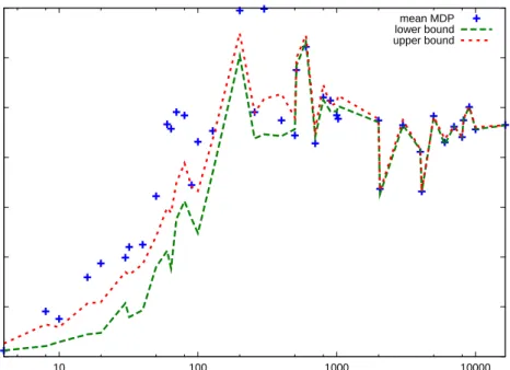
Figure 1: Illustration of upper and lower bounds on the value function, averaged over all states, as more observations are acquired. It can be seen that the , mean MDP value (crosses) is far from the bounds initially. The bounds were calculated by taking the empirical mean of 1000 MDP sam-ples from the current belief.

(18)

of the mean MDP does not generally equal the expected value of the BAMDP:

Vµ¯π_ξ6=E[Vπ|ξ].

Nevertheless, the stationary policy that is optimal with respect to the mean MDP can be used to evaluate the right hand side forπ=πµ∗¯, which will hopefully result in a relatively tight lower bound. This is illustrated in Figure 1, which displays up-per and lower bounds on the BAMDP value function as observations are acquired in a simple maze task.

If the beliefsξ can be expressed in closed form, it is easy to calculate the mean transition distribution and the mean reward fromξ. For discrete state spaces, transitions can be expressed as multinomial distributions, to which the Dirichlet density is a conjugate prior. In that case, for Dirichlet parameters_{ψ_ij,a(ξ): i,j_∈

S_,_a_∈A_}_{, we have} ¯ µ_ξ(s′|s,a) = ψ s,a s′ (ξ) ∑i∈Sψ_is,a(ξ) (5.11) Similarly, for Bernoulli rewards, the corresponding mean model arising from the beta prior with parameters{αs,a₍_ξ₎_,_βs,a₍_ξ₎_{: s}_∈_S_,_a_∈_A_}_{is E}_[_r_|_s_,_a_,_µ_¯

ξ] =

αs,a₍_ξ₎_/₍_αs,a₍_ξ_{) +}_βs,a₍_ξ₎₎_{. Then the value function of the mean model can be}

found with standard value iteration.

5.4.2 Bounds with high probability

In general, neither the upper nor the lower bounds cannot be expressed in closed form. However, the integral can be approximated via Monte Carlo sampling.

Let us be in some hyper-stateω= (s,ξ). We can obtain c MDP samples from the belief atω: µ1, . . . ,µc∼ξ(µ). In order to estimate the upper bound, for

eachµkwe can derive the optimal policyπ∗(µk)and estimate its value function

˜

v∗_k,Vπ∗(µk)

µk ≡Vµ∗k. We may then average these samples to obtain

ˆ v∗_c(ω),1 c c

∑

k=1 ˜ v∗_k(s), (5.12)

where s is the state at hyper-stateω. Let ¯v∗(ω) =R

Mξ(µ)Vµ∗(s)dµ. It holds that limc→∞[vcˆ ] =v¯∗(ω)and that E[vcˆ ] =v¯∗(ω). Due to the latter, we can apply a Hoeffding inequality P(|vˆ∗_c(ω)−v¯∗(ω)|>ε)<2 exp − 2cε 2 (Vmax−Vmin)2 , (5.13)

thus bounding the error within which we estimate the upper bound. For rt∈[0,1]

and discount factorγ, note that Vmax−Vmin≤1/(1−γ).

The procedure for the lower bound is identical, but we only need to estimate the value ˜vk,V

π∗₍µ¯_ξ)

µk of the mean-MDP-optimal policyπ∗(µ¯ξ)for each one of

the sampled MDPsµk. Thus we obtain a pair of high probability bounds for any

BAMDP node.

5.5 Discussion and related work

Employing the above bounds together with efficient search methods [Coquelin and Munos, 2007; Dimitrakakis, 2008, 2009; Hren and Munos, 2008] is a promising direction. Even when the search is efficient, however, the complexity remains prohibitive for large problems due to the high branching factor and the dependency on the horizon.

(19)

Poupart et al Poupart et al. [2006] have proposed an analytic solution to Bayesian reinforcement learning. They focus on how to efficiently approximate (5.7). More specifically, they use the fact that the optimal value function is the upper envelope of a set of linear segments

Vt∗,T(ωt) =max α∈Γα(ωt), with α(ωt) = Z Mξt(µ)α(st,µ)dµ.

They then show that the k+1-horizonα-function can be computed from the k-horizonα-function via the following backwards induction:

α(ωt) =

∑

i µ(st+1=i|st,a∗(ωt))[E(R|st+1=i,st,a∗(ωt)) +γα(ωi,a ∗(ω) t+1 )], (5.14) Vk+1(ω) = max a∈Γk+1α(ω), (5.15)

whereω_ti₊₁denotes the augmented state resulting from starting atωt, taking action a∗(ωt)and transiting to the MDP state i. However, the complexity of this process

is still exponential with the planning horizon. For this reason, the authors use a projection of theα-functions. This is performed on a set of belief points selected via sampling a default trajectory. The idea is that one may generalize from the set of sample beliefs to other, similar, belief states. In fact, the approximate value function they derive is a lower bound on the BAMDP value function. It is an open question whether or when the bounds presented here are tighter.

At this point, however, it is unclear under what conditions efficient online methods would outperform approximate analytic methods. Perhaps a combination of the two methods would be of interest: i.e. using the online search and bounds in order to see when the point-based approximation has become too inaccurate. The online search could also be used to sample new belief points.

It should be noted that online methods break down whenγ→1 because the belief tree can not in general be expanded to the required depth. In fact, the only currently known methods which are nearly optimal in the undiscounted case are based on distribution-free bounds Auer et al. [2008]. Similarly to the bandit case, it is possible to perform nearly optimally in an unknown MDP by considering up-per confidence bounds on the value function. Auer et al [Auer et al., 2008] in fact give an algorithm which achieves regret O(D_|S_|p

|A_|T)after T steps for any unknown MDP with diameter5D. In exactly the same way as the Bayesian

approach, the algorithm maintains countsΨover observe state-action-state tran-sitions. In order to obtain an optimistic value function, the authors consider an augmented MDP which is constructed from a set of plausible MDPs M, where M is such that P(Ψ|µ∈/M)<δ. Then, instead of augmenting the state space, they augment the action space by allowing the simultaneous choice of actions a∈A and MDPsµ_∈M. The policy is then chosen by performing average value

itera-tion [c.f. Puterman, 2005] in the augmented MDP.

There has not been much work yet for Bayesian methods in the undiscounted case, with the exception of Bernoulli bandit problems Kelly [1981]. It may well be that in fact naive look-ahead methods are impractical. In order to achieve

O(D|S_|p

|A_|_T₎_{regret with online methods Dimitrakakis [2009] requires an} in-stantaneous regretεtsuch that∑Tt εt<

√

T ,⇒εt<1/√t. If we naively bound our

instantaneous regret by discounting, then that would require our horizon to grow 5_{Intuitively, the maximin expected time needed to reach any state from any other state, where the max}

(20)

with rate O(log1/γ√t/(1−γ)), something which seems impractical with current online search techniques.

6 Partial observability

A useful extension of the MDP model can be obtained by not allowing the agent to directly observe the state of the environment, but an observation variable otthat

is conditioned on the state. This more realistic assumption is formally defined as follows:

Definition 6.1 (Partially observable Markov decision process) A partially observ-able Markov decision processµ(POMDP) is defined as the tupleµ= (S_,A_,O_,T_,R₎

comprised of a set of observationsO_{, a set of states} S_{, a set of actions} A_,

a transition-observation distributionT conditioned the current state and action

µ(st+1=s′,ot+1=o|st=s,at=a)and a reward distributionR, conditioned on

the state and actionµ(rt+1=r|st=s,at=a), with a∈A, s,s′∈S, o∈O, r∈R.

We shall denote the set of POMDPs asM_P. For POMDPs, it is often assumed that one of the two following factorizations holds:

POMDPs are formally identical to BAMDPs. More specifically, BAMDPs cor-respond to a special case of a POMDP in which the state is split into two parts: One fully observable dynamic part and one unobservable, continuous, but stationary part, which models the unknown MDP. Typically, however, in POMDP applica-tions the unobserved part of a state is dynamic and discrete.

The problem of acting optimally in POMDPs has two aspects. The first is state estimation, and the second is acting optimally given the estimated state. As far as the first part is concerned, given an initial state probability distribution, updating the belief for a discrete state space amounts to simply maintaining a multinomial distribution over the states. However, the initial state distribution might not be known. In that case, we may assume an initial prior density over the multinomial state distribution. It is easy to see that this is simply a special case of an unknown state transition distribution, where we insert a special initial state which is only visited once. We shall, however, be concerned with the more general case of full exploration in POMDPs, where all state transition distributions are unknown.

6.1 Belief POMDPs

It is possible to create an augmented MDP for POMDP models, by endowing them with an additional belief state, in the same manner as MDPs. However now the belief state will be a joint probability distribution overM_P_andS_{. Nevertheless,} each(at,ot+1)pair that is observed leads to a unique subsequent belief state. More formally, a belief-augmented POMDP is defined as follows:

Definition 6.2 (Belief POMDP) A Belief POMDPν (BAPOMPD) is an MDP

ν= (Ω,A_,O_,T′_,R′₎_whereΩ₌G_×B_{, where}G _{is the set of probability}

(21)

state transition and reward distributions conditioned on the belief stateξtand the action atsuch that the following factorizations are satisfied for allµ∈M_P,ξ_t_∈B

p(st+1|st,at,st−1, . . . ,µ) =µ(st+1|st,at) (6.3)

p(ot|st,at,ot−1, . . . ,µ) =µ(ot|st,at) (6.4)

p(ξt+1|ot+1,at,ξt) =

Z

M_Pp(ξt+1|µ,ot+1,at,ξt)ξt+1(µ|ot+1,at,ξt)dµ (6.5)

We shall denote the set of BAPOMDPs withM_BP_{. Again, (6.5) simply assures that} the transitions in the belief-POMDP are well-defined. The Markov stateξt(µ,st)

now jointly specifies a distribution over POMDPs and states.6As in the MDP case, in order to be able to evaluate policies and select actions optimally, we need to first construct the BAPOMDP. This requires calculating the transitions from the current belief state to subsequent ones according to our possible future observations, as well as the probability of those observations. The next section goes into this in more detail.

6.2 The belief state

In order to simplify the exposition, in the following we shall assume firstly that each POMDP has the same number of states. Thenξ(st=s|µ)describes the prob-ability that we are in state s at time t given some beliefξand assuming we are in the POMDPµ. Similarly,ξ(st=s,µ)is the joint probability given our belief. This joint distribution can be used as a state in an expanded MDP, which can be solved via backward induction, as will be seen later. In order to do this, we must start with an initial beliefξ0and calculate all possible subsequent beliefs. The belief at time t+1 depends only on the belief time t and the current set of observations

rt+1,ot+1,at. Thus, the transition probability fromξttoξt+1is just the probability of the observations according to our current belief,ξt(rt+1,ot+1|at). This can be calculated by first noting that given the model and the state, the probability of the observations no longer depends on the belief, i.e.

ξt(rt+1,ot+1,|st,at,µ) =µ(rt+1,ot+1|at,st) =µ(rt+1|at,st)µ(ot+1|at,st). (6.6) The probability of any particular observation can be obtained by integrating over all the possible models and states

ξt(rt+1,ot+1|at) = Z

M_P

Z

Sµ(rt+1,ot+1|at,st)ξt(µ,st)dµdst. (6.7) Given that a particular observation is made from a specific belief state, we now need to calculate what belief state it would lead to. For this we need to compute the posterior belief over POMDPs and states. The belief over POMDPs is given by

ξt+1(µ),ξt(µ|rt+1,ot+1,at,) (6.8) =ξt(rt+1,ot+1,at|µ)ξt(µ) ξt(rt+1,ot+1,at) (6.9) =ξt(µ) Z ZZ Sµ(rt+1,ot+1,at|st+1,st)ξt(st+1,st|µ)dst+1dst (6.10)

6_{The formalism is very similar to that described in Ross et al. [2008a], with the exception that we do not}

Efficient methods for near-optimal sequential decision making under uncertainty