713
FORECASTING LINEAR TIME SERIES MODELS WITH
HETEROSKEDASTIC ERRORS IN A BAYESIAN APPROACH
Esmail Amiri
Imam Khomeini International University, Ghazvin, Iran, [email protected] ABSTRACT. A study was conducted to compare the forecasting perfor-mance of four models, namely Stochastic Volatility (SV), Generalized Au-toregressive Conditional Heteroskedasticity (GARCH), AuAu-toregressive with GARCH errors (AR-GARCH) and Autoregressive with SV errors (AR-SV). Bayesian approach and Markov Chain Monte Carlo (MCMC) simulation methods are applied to estimate the parameters of the models and their pre-dictive densities; using three time series data (daily Euro/US Dollar, British Pound/US Dollar and Iranian Rial/US Dollar exchange rates). Out-of-sample analysis through cumulative predictive Bayes factors clearly showed that modeling regression residuals heteroskedastic, substantially improves predictive performance, especially in turbulent times. A direct comparison of SV and vanilla GARCH(1,1) indicated that the former performs better in terms of predictive accuracy.
Keywords: Bayesian inference, Markov chain Monte Carlo (MCMC), het-eroskedasticity, financial time series
INTRODUCTION
The stochastic volatility (SV) model introduced by Tauchen and Pitts (1983) and Taylor (1982) is used to describe financial time series. It offers an alternative to the ARCH-type models of Engle (1982) and Bollerslev (1986) for the well-documented time-varying volatili-ty exhibited in many financial time series. The SV model provides a more realistic and flexi-ble modeling of financial time series than the ARCH-type models, since it essentially in-volves two noise processes, one for the observations, and one for the latent volatilities. The so-called observation errors account for the variability due to measurement and sampling errors whereas the process errors assess variation in the underlying volatility dynamics (see, for example, Taylor (1994), Ghysels et al. (1996), and Shephard (1996) for the comparative advantages of the SV model over the ARCH-type models).
Unfortunately, classical parameter estimation for SV models is difficult due to the intrac-table form of the likelihood function. In the literature, a variety of frequentist estimation methods have been proposed for the SV model, including generalized method of moments (Melino and Turnbull (1990), Sorensen (2000)), quasi-maximum likelihood (Harvey et al., 1994), efficient method of moments (Gallant et al., 1997), simulated maximum likelihood (Danielsson (1994), Sandmann and Koopman (1998)), and approximate maximum likelihood (Fridman and Harris, 1998). A Bayesian analysis of the SV model is complicated due to mul-tidimensional integration problems involved in posterior calculations. These difficulties with posterior computations have been overcome, though, with the development of Markov chain Monte Carlo (MCMC) techniques (Gilks et al., 1996) over the last two decades and the ready
714
availability of computing power. MCMC procedures for the SV model have been suggested by Jacquier et al. (1994), Shephard and Pitt (1997), and Kim et al. (1998).
In Bayesian estimation algorithms, the stochastic volatility specification is computational-ly tractable. In addition, studies such as Clark (2011) and Carriero, Clark, and Marcellino (2012) have shown that it is effective for improving the accuracy of density forecasts from AR models.
In a Bayesian approach our aim is to compare the forecasting performance of two nonline-ar models, namely GARCH and SV models to linenonline-ar autoregressive models with GARCH and SV errors. To illustrate model comparison and evaluation, we fit the models to the daily log of three exchange rate time series, namely EUR/USD, GBP/USD and IRR/USD. MCMC simulation methods are employed to estimate the parameters of the models and their predic-tive densities. The predicpredic-tive performance of the models is assessed through their predicpredic-tive densities and likelihood evaluations.
The paper proceeds as follows. The second section is devoted to model specification and estimation, the third section describes the data, the fourth section is allocated to empirical results and the last section presents conclusion.
MODEL SPECIFICATION AND ESTIMATION
We begin by briefly introducing the models and specifying the notation used in the re-mainder of the paper. Furthermore, an overview of Bayesian parameter estimation via Mar-kov chain Monte Carlo (MCMC) methods is given.
The GARCH and SV models
Let T
n
y y y
y ( 1, 2,..., ) be a vector of returns with mean zero. The intrinsic feature of the SV model is that each observation
y
tis assumed to have its “own" contemporaneous variancet h
e , thus relaxing the usual assumption of homoskedasticity. In order to make the estimation of such a model feasible, this variance is not allowed to vary unrestrictedly with time. Rather, its logarithm is assumed to follow an autoregressive process of order one. Note that this fea-ture is fundamentally different to GARCH-type models where the time-varying volatility is assumed to follow a deterministic instead of a stochastic evolution.
The SV model can thus be conveniently expressed in hierarchical form. In its centered pa-rameterization, it is given through
) , 0 ( ~ | ht t t h N e y , (1)
)
),
(
(
~
,
,
,
|
2 1 1 t t th
N
h
h
, (2)))
1
/(
,
(
~
,
,
|
2 2 0N
h
, (3)where N( , 2) denotes the normal distribution with mean and variance 2. We re-fer to
(
,
,
)
Tas the vector of parameters: the level of log-variance , the persistence of log-variance , and the volatility of log-variance . The processh
(
h
0,
h
1,...,
h
n)
ap-pearing in Eq. (2) and Eq. (3) is unobserved and usually interpreted as the latent time-varying volatility process (more precisely, the log-variance process). Note that the initial stateh
0ap-715
pearing in Eq. (3) is distributed according to the stationary distribution of the autoregressive process of order one.
The Bayesian Normal Linear Model
The Bayesian normal linear model withnobservations and k p 1 predictors, given through ) , ( ~ , | N y (4)
Here, y denotes the n 1 vector of responses, X is the n p design matrix containing
ones in the first column and the predictors in the others, and ( 1, 2,..., 1)
p stands for
the p 1 vector of regression coefficients. The simplest specification of the error covariance matrix in Equation 5 is given by 2 , where I denotes the n-dimensional unit matrix. This specification is used in many applications and commonly referred to as the linear regression model with homoskedastic errors.
The Bayesian Normal Linear Model with SV Errors
Instead of homoskedastic errors, we now specify the error covariance matrix in Eq. (4) to be diag(eh1,...,ehn), thus introducing nonlinear dependence between the observations
due to the AR(1)-nature of h.
The Bayesian Normal Linear Model with GARCH Errors
The Bayesian normal linear model with GARCH(1,1) errors can be specified through Eq. (4) with ( 2,..., 2) 1 n diag and 2 21 2 1 1 0 2 ~ t t t y , where t 1,...,n and ~yt 1
denotes the past “residual”, i.e, the (t 1)th element of y~ y .
Prior distribution
For the SV model, a prior distribution for the parameter vector needs to be specified. Following Kim et al. (1998), we choose independent components for each parameter, i.e.,
) ( ) ( ) ( ) ( p p p p .
The level Ris equipped with the usual normal prior ~N(b ,B ). In practical ap-plications, this prior is usually chosen to be rather uninformative, e.g., through setting b 0 and B 1000 for daily log returns.
For the persistence parameter ( 1,1), we choose( 1)/2~ (a0,b0), implying
1 1 0 0 0 0 ) 2 1 ( ) 2 1 ( ) , ( 2 1 ) ( a b b a p , (5)
716
where a0 andb0 are positive hyperparameters and
1 0 1 1( 1) ) , (x y tx t y dt denotes the
beta function. Clearly, the support of this distribution is the interval ( 1,1); thus, stationarity
of the autoregressive volatility process is guaranteed. Its expected value and variance are giv-en through the expressions
)
1
(
)
(
4
)
(
,
1
2
)
(
0 0 2 0 0 0 0 0 0 0b
a
b
a
b
a
V
b
a
a
E
.For the volatility log-variance R , we choose 2 (1/2,1/2 )
1
2 G
.
DATA
We use the daily price of 1 EUR in USD , 1 GBP in USD and 1 IRR in USD from January
3, 2000 to December 31, 2014, denoted by p (p1,p2,...,pn). We investigate the
develop-ment of log levels by regression.
EMPERICAL RESULTS
In order to reduce prior influence, the first 1000 days are used as a training set only and the evaluation of the predictive distribution starts at t = 1001, corresponding to December 4,
2003. WinBUGSsoftware is used to carry out the computations.
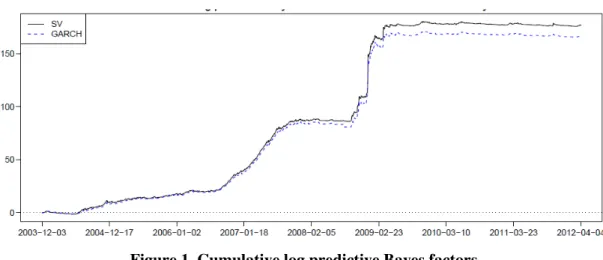
Figure 1. Cumulative log predictive Bayes factors
Figure 1 shows cumulative log predictive Bayes factors in favor of the model with SV re-siduals for EUR/USD time series. Values greater than zero mean that the model with GARCH/SV residuals performs better out of sample up to this point in time.
717
Table 1. Cumulative predictive log likelihoods for GARCH, SV, AR(1) models with different error assumptions, applied to the logarithm of EUR/USD, GBP/USD and
IRR/USD
Currency GARCH SV AR-SV
AR-GARCH AR
EUR/USD 7862 7865 7878 7868 7701
GBP/USD 8538 8542 8568 8549 8218
IRR/USD 8870 8875 9011 8880 8255
Table 1 presents cumulative predictive log likelihoods for GARCH(1,1), SV, AR(1) mod-els with different error assumptions, applied to the logarithm of EUR, GBP and IRR ex-change rates. AR-SV is strongly favored in all cases.
CONCLUSION
In a Bayesian approach we have compared forecasting performance of four time varying volatility models. The set of models includes GARCH, SV, AR-GARCH and AR-SV models. Markov Chain Monte Carlo (MCMC) simulation methods are employed to estimate models parameters. Real-time forecasts of log level EUR / USD, GBP/USD and IRR/ USD exchange rates are produced. For the three time series, out-of-sample analysis through cumulative pre-dictive Bayes factors clearly showed that modeling regression residuals heteroskedastically substantially improves predictive performance, especially in turbulent times. A direct compar-ison of SV and vanilla GARCH(1,1) indicated that the former performs better in terms of predictive accuracy. Further research needs to be done to devise new efficient sampling algo-rithms.
REFERENCES
Amisano, G. J. (2010). Comparing and Evaluating Bayesian Predictive Distributions of Asset Returns.
International Journal of Forecasting, 26(2), 216-230.
Andrea, C., Clark, T.E., & Marcellino, M. (2012). Common Drifting Volatility in Large Bayesian VARs. Manuscript, Federal Reserve Bank of Cleveland.
Bollerslev, T .(1986). Generalized Autoregressive Conditional Heteroskedasticity. Journal of Econo-metrics, 31(3), 307-327.
Clark, T. E. (2011). Real-Time Density Forecasts From BVARs With Stochastic Volatility. Journal of Business and Economic Statistics, 29, 327-341.
Danielsson, J. (1994). Stochastic volatility in asset prices: estimation with simulated maximum likely hood. Journal of Econometrics, 64, 375–400.
Engle, R.F. (1982). Autoregressive Conditional Heteroscedasticity with Estimates of the Variance of United Kingdom Ination. Econometrica, 50(4), 987-1007.
Fridman, M. & L. Harris (1998). A maximum likelihood approach for non-Gaussian stochastic volatili-ty models. Journal of Business and Economic Statistics 16, 284–91.
Gallant, A. R., Hsie, D., & Tauchen, G. (1997). Estimation of stochastic volatility models with diag-nostics. Journal of Econometrics, 81, 159–92.
718
Ghysels, E., Harvey, A.C., & Renault, E. (1996). Stochastic Volatility. In G.S. Maddala, C.R. Rao (eds.), Handbook of Sttaistics: Statistical Methods in Finance, 14, 119-191.
Gilks, W. R., Richardson, S., & Spiegelhalter, D. J. (1996). Markov Chain Monte Carlo in Practice. London: Chapman & Hall.
Harvey, A. C., Ruiz, E., & Shephard, N. (1994). Multivariate stochastic variance models. Review of Economic Studies, 61, 247–64.
Jacquier, E., Polson, N.G., Rossi, P.E. (1994). Bayesian Analysis of Stochastic Volatility Models. Journal of Business & Economic Statistics, 12(4), 371-389.
Kim, S., Shephard, N., & Chib, S. (1998). Stochastic Volatility: Likelihood Inference and Comparison with ARCH Models. Review of Economic Studies, 65(3), 361-393.
Melino, A. & Turnbull, S. M. (1990). Pricing foreign currency options with stochastic volatility. Jour-nal of Econometrics, 45, 239–65.
Meyer, R., & Yu, J. (2000). BUGS for a Bayesian Analysis of Stochastic Volatility Models. The Econ-ometrics Journal, 3(2), 198-215.
Shephard, N. (1996). Statistical aspects of ARCH and stochastic volatility. In Cox, D. R., Hinkley, D.V., and Barndorff-Nielson, O. E. (eds), Time Series Models in Econometrics, Finance and Other Fields, (pp. 1–67). London: Chapman & Hall.
Sorensen, M. (2000). Prediction based estimating equations. The Econometrics Journal, 3, 123–147. Tauchen, G. & Pitts, M. (1983). The price variability-volume relationship on speculative markets.
Econometrica, 51, 485–505.
Taylor, S. J (1994). Modelling stochastic volatility. Mathematical Finance, 4, 183-204.
Taylor, S.J. (1982). Financial Returns Modelled by the Product of Two Stochastic Processes: A Study of Daily Sugar Prices 1691-79. In OD Anderson (ed.), Time Series Analysis: Theory and Prac-tice,1, pp.203-226. North-Holland, Amsterdam.
Wermuth, N., & Lauritzen, S. L. (1990). On substantive research hypothesis, conditional independence graphs and graphical chain models (with discussion). Journal of the Royal Statistical Society Se-ries B, 38, 21–72.