Titl e
P r e d i c ti n g Glo b al Te m p e r a t u r e An o m aly: A D efi ni tiv e
I nv e s ti g a ti o n U si n g a n E n s e m b l e of Tw elv e C o m p e ti n g
F o r e c a s ti n g M o d el s
Ty p e
Ar ticl e
U RL
h t t p s :// u al r e s e a r c h o nli n e . a r t s . a c . u k/i d/ e p ri n t/ 1 2 9 3 7 /
D a t e
2 0 1 8
Cit a ti o n
H a s s a n i, H . a n d Silv a, E. S. a n d G u p t a , R. a n d D a s , S.
( 2 0 1 8 ) P r e d i c ti n g Glo b al Te m p e r a t u r e Ano m aly: A
D efi ni tiv e I nv e s ti g a tio n U si n g a n E n s e m b l e of Tw elv e
C o m p e ti n g F o r e c a s ti n g M o d el s. P h y si c a A: S t a ti s ti c al
M e c h a n i c s a n d it s Ap plic a ti o n s , 5 0 9 . p p . 1 2 1-1 3 9 .
C r e a t o r s
H a s s a n i, H . a n d Silv a, E. S. a n d G u p t a , R. a n d D a s , S.
U s a g e G u i d e l i n e s
Pl e a s e r ef e r t o u s a g e g u i d eli n e s a t
h t t p :// u al r e s e a r c h o n li n e . a r t s . a c . u k / p olici e s . h t m l
o r a l t e r n a tiv ely c o n t a c t
u a l r e s e a r c h o n li n e @ a r t s . a c . u k
.
Lic e n s e : C r e a tiv e C o m m o n s Att ri b u ti o n N o n-c o m m e r ci al N o D e riv a tiv e s
U nl e s s o t h e r wi s e s t a t e d , c o p y ri g h t o w n e d b y t h e a u t h o r
Predicting Global Temperature Anomaly: A Definitive
Investigation Using an Ensemble of Twelve Competing
Forecasting Models
∗ Hossein HassaniResearch Institute of Energy Management and Planning University of Tehran, Iran. Email: [email protected].
Emmanuel Sirimal Silva
Fashion Business School, London College of Fashion, University of the Arts London, UK. Email: [email protected].
Rangan Gupta
Department of Economics, University of Pretoria, Pretoria, 0002, South Africa. Email: [email protected].
Sonali Das
Advanced Mathematical Modelling, Modelling and Digital Science,
Council for Scientific and Industrial Research, P.O. Box 395, Pretoria, 0001, South Africa. Email: [email protected]. The School of Statistics and Actuarial Science, University of the Witwatersrand, Johannesburg, 2000, South Africa
and
Department of Statistics, Nelson Mandela University, Port Elizabeth, 6031, South Africa.
June 25, 2018
Abstract
In this paper we analyze whether (anthropometric) CO2can forecast global temperature anomaly (GT) over an annual out-of-sample period of 1907-2012, which corresponds to an initial in-sample of 1880-1906. For our purpose, we use 12 parametric and nonparametric univariate (of GT only) and multivariate (including both GT and CO2) models. Our results show that the Horizontal Multivariate Singular Spectral Analysis (HMSSA) techniques (both Recurrent (-R) and Vector (-V)) consistently outperform the other competing models. More importantly, from the performance of the HMSSA-V model we find conclusive evidence that CO2 can forecast GT, and also predict its direction of change. Our results highlight the superiority of the nonparametric approach of SSA, which in turn, allows us to handle any statistical process: linear or nonlinear, stationary or stationary, Gaussian or non-Gaussian.
JEL Codes: C22; C32; C53; Q53; Q54.
Keywords: CO2emissions; Forecasting; Global temperature anomaly; Univariate and
multivari-ate models.
1
Introduction
The climate change debate consists of players who, in the absence of accessible evidence-based and objective information, may resort to decisions based on perceptions and even possibly po-litical agendas (Khandekar et al., 2005). The debate gets even more aggressive when global
∗We would like to thank five anonymous referees for many helpful comments. However, any remaining errors
warming is discussed in relation to anthropometric carbon dioxide (CO2) emissions (Solomon et
al., 2009; Fildes and Kourentzes, 2011; McMillan and Wohar, 2013; Beenstock et al., 2016). Global warming has been accepted as a reality. For example, see Green and Armstrong (2007) and more recently, Dergiades et al., (2016) for a detailed discussion based on the time-series rela-tionship between global temperatures and emissions. The purpose of this paper is to undertake a rigorous investigation of well-established datasets for global temperature (GT) and CO2 us-ing a suite of forecastus-ing models in an attempt to identify, possibly, a sus-ingle model that can be prescribed for forecasting GT. Specifically, we consider 12 time-series models for forecasting GT from both parametric and nonparametric paradigms. These 12 models include 7 univariate models and 5 multivariate models namely: Random Walk (RW), Autoregressive (AR), Autore-gressive Integrated Moving Average (ARIMA), Exponential Smoothing (ETS), Neural Networks (NN), Fractionalized ARIMA (ARFIMA), Box-Cox transformation, ARMA errors, Trend and Seasonal components (BATS), Bayesian Autoregression (BAR), Vector Autoregression (VAR), Bayesian Vector Autoregression (BVAR), Singular Spectrum Analysis (SSA) and Multivariate Singular Spectrum Analysis (MSSA). Note that, our primary focus in this paper is forecast-ing GT usforecast-ing the information contained in CO2 using the SSA approach, due to its modeling
flexibility advantages discussed in the next segment. However, given that a forecasting exercise requires competing models, we choose a wide array of linear and nonlinear versions of univariate and multivariate models most commonly used in the forecasting literature.
Our sample covers the entire period of 1880-2012, with an out-of-sample period of 1907-2012 (based on an initial in-sample period of 1880 to 1906 - note that this initial in-sample period is incremented by one year and models are re-estimated except in the case of RW and SSA models). The start and end points of the analysis are purely driven by data availability at the time of writing this paper, but the choice of the out-of-sample period is determined by the earliest possible break date detected (based on the Bai and Perron (2003) tests of multiple structural breaks) in the relationship between GT and CO2, which happened to be 1906. Since, we estimate
our linear models recursively over the out-of-sample period, we are able to accommodate the change in the parameter estimates of the model while producing our forecasts. This approach makes the linear and nonlinear approaches comparable, with both types of model being now able to correct misspecication due to breaks either by structural design or through recursive estimation.
This paper makes several important contributions: (i) this paper makes the first attempt to provide a comprehensive comparison of models for forecasting GT available in the literature; (ii) it marks the introductory application of models such as BATS, SSA and MSSA for forecasting GT; and, (iii) finally, we use a new and automated MSSA forecasting algorithm for generating out-of-sample forecasts for GT. The SSA and MSSA models contribute to the literature on forecasting GT by decomposing GT for denoising and signal extraction prior to forecasting, in addition to the multivariate analysis of both GT and CO2 in the case of MSSA. Moreover, this
automated MSSA forecasting algorithm is optimised based on minimising a loss function. As such, it ensures the overall MSSA process is less labour intensive as it does away with the need for having to analyse eigenvectors individually in order to differentiate between signal and noise. Also, it can show the best MSSA model for forecasting any given data set in-sample and can therefore be used in future forecasting studies as well. To the best of our knowledge, barring the two studies of Fildes and Kourentzes (2011), and McMillan and Wohar (2013), all other papers in this area involving time series analysis have analyzed these two variables separately in univariate settings.1
1The reader is referred to McMilan and Wohar (2013) for a detailed literature review in this regard, which primarily involves analysis of unit root and persistence properties of these two variables.
Our results show that the nonparametric approach of SSA consistently outperform the other competing models. More importantly, from the performance of the SSA models, we find conclu-sive evidence that CO2 can forecast GT, and also predict its direction of change. The remainder
of the paper is organised as follows: in Section 2, we discuss the literature review, while Section 3 presents a detailed description of the 12 forecasting models investigated with extra emphasis on the SSA and MSSA techniques. In Section 4, we outline the datasets used and the metrics used for the evaluation of the models, with estimations conducted in either R or RATS. In Section 5, we present an in-depth analyses of the results in our quest to identify the best model for our purpose, while in Section 6, we present a discussion. Finally, we present some concluding remarks on the investigation undertaken in Section 7.
2
Literature Review
Note, the relationship between CO2 and GT is primarily analyzed using Coupled
Atmospheric-Ocean General Circulation Models (AOGCMs) of the United Nations Intergovernmental Panel on Climate Change (IPCC). While the AOGCM is the primary framework, smaller models focusing on certain aspects of the world’s climate are also used. Besides the small-and large-scale AOGCMs, there is also a statistical approach, whereby models are estimated directly from observations. But the latter as indicated above, is limited.
The AOGCMs comprise of systems of partial differential equations based on the basic laws of physics, fluid motion and chemistry, aimed at capturing the dynamics of the atmosphere and oceans. Given a set of initial and boundary conditions (which include emissions of atmo-spheric gases such as CO2 and volcanic eruptions), these models use a three-dimensional grid
to simulate the dynamics and to produce time-varying outputs such as global temperature (and precipitation) (Fildes and Kourentzes, 2011).2 The advantage of these types of models is that,
if the model represents the physical laws accurately, it should be possible to simulate scenarios which have not been seen in the past (McSharry, 2011). However, there are serious limitations to this approach: (a) Attempting to describe the planet using a 200 km grid implies a limited ability to simulate the subgrid-scale dynamics of clouds, aerosols and turbulence adequately; (b) Climate modellers use parameterisation techniques in an attempt to make up for the problems of resolution, but the varying approaches yield different results (Stainforth et al., 2005); (c) Uncertainties also arise from an incomplete understanding of the interchange of CO2 between
the oceans, atmosphere and biosphere (McSharry, 2011), and; (d) Uncertainty results from the judgemental approaches employed in constructing these models (Stainforth et al., 2007).
Given the above-mentioned issues, papers like that of Fildes and Kourentzes (2011), and McMillan and Wohar (2013), have pursued a statistical approach using historical observations, and provide a means of representing patterns in the data based on linear, nonlinear and non-parametric methods. The forecasting performances of statistical models obviously depend on the extent to which the future looks like the past. So, whereas AOGCMs are governed by laws of physics, fluid motion and chemistry, the statistical models are dependent on the quality of the data. Hence, there is an argument that statistical models have little value in forecasting global temperatures, because the rising CO2 emissions mean that the future is unlikely to be similar
to the past (McSharry, 2011).
Instead of completely dismissing statistical approaches, Fildes and Kourentzes (2011), based on established encompassing tests, show that there are advantages of combining a specific
2It must be pointed out that, AOGCMs actually use CO
2 concentration as a forcing variable, which in turn, depends on the pattern of emissions, with the representative concentration pathways (RCPs) used for forecasts being based on different emission scenarios.
AOGCM (namely United Kingdom Meteorological Office decadal climate prediction system, known as DePreSys, as developed by Smith et al., (2007)) with linear and nonlinear time series models (namely, the combined forecast obtained from random walk; single, Holt and damp-ened trend exponential smoothings; autoregressive; univariate and multivariate (including CO2
emissions) neural networks). While DePreSys provides superior short-term forecasting (one- to four-years-ahead), gains in forecast accuracy were achieved for up to 10-year forecasts using an univariate Holt exponential smoothing model and a multivariate neural network model which included CO2 as a predictor variable.3 McMillan and Wohar (2013), based on VAR and
Gener-alized Method of Moments (GMM) approaches conclude that CO2 has a weak relationship with
GT, both in terms of in-sample causality tests and an out-of-sample exercise of predicting the last observation in their sample. This could, however, be a result of uncaptured nonlinearity in the relationship between these two variables, which Fildes and Kourentzes (2011) emphasized upon, and which we show to exist in the discussion that follows in the results segment of the paper.4
Against this backdrop, in this paper we basically aim to understand better the underlying form of nonlinearity in the relationship between GT and CO2 emissions by conducting an
out-of-sample forecasting exercise, using univariate and multivariate versions of linear and nonlinear models. In the process, we look at a nonparametric approach using the SSA technique, over and above the neural network model. We also follow the recommendations of McSharry (2011), who suggests that while the neural network approach is a flexible one, it is possible to improve the underlying nonlinearity by using alternative model specifications. Note that our approach is purely based on a time series analysis, and excludes climate models. Hence, as part of future research, as in Fildes and Kourentzes (2011), it would be interesting to pursue forecast combinations of the SSA models that we develop and AOGCMs, if and when forecast data from the latter set of models could be accessed. Note that the decision to rely on an out-of-sample rather than an in-sample predictability exercise to gauge the relationship between CO2 and
global temperature is motivated out of the belief that: “The ultimate test of any predictive model is its out-of-sample performance” (Campbell, 2008). Since we only use a part of the data to fit various models, and produce predictions for the remaining part of the sample period. Using full-sample information allows even liner models to pick up nonlinearity in the data. However, this is not the case, when we spilt the data into and out-of-sample periods, since good in-sample predictions does not guarantee the same for forecasting over an out-of-in-sample period. This is because, a particular model might be misspecified over the out-of-sample period due to limited in-sample information.
At this stage, it is important to emphasize the reasons to use the SSA technique in forecasting
3Fildes and Kourentzes (2011), also compared local temperature forecasts at six locations to show that the ten-year-ahead forecasts of the AOGCMs were worse than forecasts from a random walk benchmark, with the exponential smoothing providing the best results. In addition, at a very long-run horizon of twenty years ahead, the multivariate neural network with CO2emissions as an explanatory variable produced superior forecasts compared to other time series models. Finally, using the CO2 concentration in the atmosphere, which is believed to be physically relevant for determining global temperatures, rather than CO2 emissions, did not improve the forecasts. 4In a somewhat connected line of research, Kaufmann and Stern (2004), and Beenstock et al., (2016) tested the historic tracking capabilities of climate models. Climate modellers use in-sample correlations to confirm the ability of climate models to track the global temperature historically. But, a high correlation though necessary, is not a sufficient condition for such confirmation, given that global temperature tends to be nonstationary. In addition, the tracking errors must also be stationary. Using cointegration tests applied to hindcast data for global temperatures generated by multiple climate change models, both Kaufmann and Stern (2004), and Beenstock et al., (2016) found that global temperature and their hindcasts, generally fail to be cointegrated. This result meant that the climate models fail to track global temperature historically in the longer run, because their tracking errors are nonstationary.
GT. SSA has recently evolved as a powerful technique in the field of time series analysis (Sanei and Hassani, 2015), besides the other standard forecasting approaches indicated above. SSA is a nonparametric technique that works with arbitrary statistical processes, whether linear or non-linear, stationary or non-stationary, Gaussian or non-Gaussian. Given that the dynamics of real time series, in our case GT, has usually gone through structural changes during the time period under consideration, one needs to make certain that the method of prediction is sensitive to the dynamical variations. Moreover, even though some might argue that the nonparametric nature of SSA/MSSA suggests little about the dynamic nature of the model, the exploitation of Takens’ theorem (Takens, 1981) in the embedding approach helps overcome this issue. In particular, MSSA succeeds in providing insights into the dynamics of the underlying system via the decomposition of delay-coordinate phase space of given multivariate time series into a set of data-adaptive orthonormal components such as trend, oscillatory patterns and noise (Ghil et al., 2002; Vautard and Ghil, 1989; Ghil and Vautard, 1991).
In addition, contrary to the standard methods of time series forecasting that assume nor-mality and stationarity of the series (though the latter is not an issue for BVAR models), as a nonparametric method, SSA makes no prior assumptions about the data, with forecasts being obtained through bootstrapping. Furthermore, SSA decomposes a series into its component parts, and reconstructs the series by leaving out the random (noise) component. Clearly then, SSA is a much more general approach that allows us to handle issues of stationarity, non-normality, non-linearity, and even seasonality, though the latter is not an issue in our annual data set. In what follows, the predictive accuracy of all forecasts are evaluated via the Root Mean Squared Error (RMSE) and Mean Absolute Error (MAE) loss functions, the direction of change criterion, and the Hassani-Silva (HS) test for predictive accuracy (Hassani and Silva, 2015) and the modified Diebold-Mariano test (Harvey et al., 1997), thus enabling a sound analysis and derivation of reliable conclusions.
3
Forecasting Models
3.1 Random Walk (RW)
The random walk model is used as a benchmark. This is because it is widely accepted that when introducing forecasting techniques for a particular purpose, it is vital that the introduced techniques are able to outperform the RW5. In brief, the RW model states that today’s GT is
the best forecast for tomorrow’s GT.
3.2 Autoregressive Integrated Moving Average (ARIMA)
In this paper we use an optimized version of ARIMA (auto-ARIMA), and provided through the forecast package6 in R. A more detailed description of the algorithm underlying auto-ARIMA can be found in Hyndman and Khandakar (2008) whilst a summarized version is available in Hassani et al. (2015b). The process for obtaining point forecasts using theRsoftware is concisely presented in Hyndman and Athanasopoulos (2013). The initial model structure and parameters for forecasting GT with ARIMA before re-estimation was ARIM A(0,0,1) with non-zero mean.
5http://robjhyndman.com/hyndsight/benchmarks/
6It should be noted that the automated algorithms in the forecast package generates a new and improved re-estimated model each time a new observation is added to the data. As such the models reported for the forecast package are the initial ones.
3.3 Exponential Smoothing (ETS)
The ETS technique in the forecast package overcomes the limitations of the Makridakis et al. (1998) algorithm pertaining to the calculation of prediction intervals. Whilst a detailed description of the ETS technique can be found in Hyndman and Athanasopoulos (2013), in brief this algorithm considers the error, trend and seasonal components along with over 30 possible options for choosing the best exponential smoothing model via optimization of initial values and parameters using Maximum Likelihood Estimator and selecting the best model based on the Akaike information criterion (AIC). In the case of GT, the model structure and parameters for forecasting GT with ETS before re-estimation was an additive ET S(A, N, N) model which is equivalent to anARIM A(0,1,1) model as linear ETS models are special cases of ARIMA model
(Hyndman and Athanasopoulos, 2013).7
3.4 Neural Networks (NN)
The NN model used in this paper is popularly referred to as nnetar and is provided through the forecast package in R. For a detailed explanation on how the nnetar model operates, see Hyndman et al. (2013). It may be noted that in all cases the selected neural network model has only k=1 hidden node,p=2 lags, with the specifications being based on annual differences of the data. The neural network takes the form
ˆ yt= ˆβ0+ k X j=1 ˆ βjψ(x ′ t.ˆγj), (1)
where xt consist ofp lags ofytand the functionψ has the logistic form
ψ(x′t.ˆγj) = [1 +exp(−γˆj0+ p X i=1 ˆ γji.yt−1)] −1j= 1, . . . , k (2)
In the neural network literature, this form is often referred to as a one hidden layer feed forward neural network model. As can be seen, the nonlinearity arises through the lagged ytentering in
a flexible way through the logistic functions of equation (1). The number of logistic functions included, namelyk, is known as the number of hidden nodes. When analysing the NN forecasting results, it is important to bear in mind that the NN results reported here are not standard as there exists no standard formulation of a NN model.
3.5 Fractionalized ARIMA Model (ARFIMA)
The ARFIMA algorithm used is also from the forecast package in R, and it automatically
estimates and selects the p and q for an ARFIMA(p,d,q) model based on the Hyndman and
Khandakar (2008) algorithm whilst d and parameters are selected based on the Haslett and
Raftery (1989) algorithm. The ARFIMA model may be written as
(1− p X i=1 φiBi)(1−B)dyt= (1 + q X i=1 φiBi)et, (3)
where B the backshift operator, p is the order of the autoregressive part, q is the number of lagged forecast errors, and d is allowed to take the form of non-integer values. The ARFIMA
model structure and parameters for forecasting GT (before re-estimation) were p = 2, d = 0, and q = 0.
3.6 Box-Cox transformation, ARMA errors, Trend and Seasonal components
(BATS)
Initially, an Exponential smoothing state space model with Box-Cox transformation, ARMA errors, Trend and Seasonal components (TBATS) model which aims to provide accurate forecasts for time series with complex seasonality was pursued via the forecast package in R. However, during the modelling process we noticed that a BATS model was found to have a better fit for this data, which is non-seasonal. A detailed description of the model and the underlying formula can be found in De Livera et al. (2011) and is therefore not reproduced here. The model structure and parameters used by the BATS model for forecasting GT before re-estimation was
BAT S(1,{0,1}), where 1 is the Box-Cox parameter and{0,1} is the damping parameter. Note
that we are permitting (additive) trend and no seasonal component.
See Appendix A1 for a discussion on the Classical Autoregressive (AR), Bayesian Autore-gressive (BAR), Vector AutoreAutore-gressive (VAR), and Bayesian Vector AutoreAutore-gressive (BVAR) Models.
3.7 Singular Spectrum Analysis (SSA)
The SSA technique is a filtering and forecasting technique which is exploited in a variety of fields (see for example, Lisi and Medio (1997), Thomakos et al. (2002), Beneki et al. (2012), Hassani et al. (2015a), Silva and Hassani (2015)). In brief, SSA seeks to filter the noise in a time series and reconstruct a less noisy signal which is then used for forecasting future data points (Hassani et al. 2015a) using only the SSA choices of window-length (L) and the number of eigenvalues r
(Hassani and Mahmoudvand, 2013). SSA also has its multivariate form which is referred to as Multivariate SSA (MSSA) and can be used for modelling and forecasting using multiple series. In comparison to SSA, MSSA is relatively new with few applications (see for example, Hassani et al. (2010c), Patterson et al. (2011), Oropeza and Sachchi (2011), Groth and Gill (2012), and Hassani et al. (2013a,b).
There are several benefits of using SSA and MSSA models. As these models are nonparamet-ric they are not bound by the parametnonparamet-ric assumptions of normality, stationarity and linearity (Hassani et al. (2013a). As such, one is able to model the data without any transformations which in turn ensures there is no loss of information (Hassani et al. 2013b). In addition, as SSA is a filtering technique, it enables users to decompose a time series in order to obtain a richer understanding of the underlying dynamics. Moreover, once the associated signal is extracted, SSA enables users to forecast the signal alone. For example, if we are interested in the trend component alone we have the option of extracting the trend from the data and then forecasting the trend.
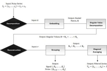
Those interested in a detailed account of the theory underlying SSA are referred to Sanei and Hassani (2015). Given that many readers are likely to be unfamiliar with the SSA, via Figure 1 we show the basic SSA process in a visual form.
In brief, the SSA technique is made up of two stages known as Decomposition and Recon-struction. Below we present the decomposition(or filtering) and reconstruction stages of SSA, and in doing so we mainly follow Sanei and Hassani (2015).
Figure 1: The basic SSA process. Stage 1: Decomposition
Consider the real-valued nonzero time series YN = (y1, . . . , yN) of sufficient lengthN. The only
choice at this stage is of the Window Length L, an integer such that 2≤L≤N.
Step 1: Embedding
Embedding is a mapping that transforms a one-dimensional time series YN = (y1, . . . , yN) into
the multi-dimensional series X1, . . . , XK with vectors Xi = (yi, . . . , yi+L−1)
′
∈RL, where K =
N −L+1. The embedding step results in the trajectory matrix X= [X1, . . . , XK] = (xij)L,Ki,j=1,
which is a Hankel matrix. Accordingly, all the elements along the diagonal i+j = const are constant (i.e., a matrix in which the (i, j)th entry depends only on i+j, that is, each skew-diagonal is constant.).
Step 2: Singular Value Decomposition (SVD)
In this step we obtain the singular value decomposition of the trajectory matrix X. Denote by
λ1, . . . , λL the eigenvalues of XX
′
in decreasing order of magnitude (λ1≥. . . λL≥0) and by
U1, . . . , UL the orthonormal system (that is, (Ui, Uj)=0 for i6= j (the orthogonality property)
and kUik=1 (the unit norm property)) of the eigenvectors of the matrixXX
′
corresponding to these eigenvalues. If we denote Vi =X
′
Ui/
√
λi, then the SVD of the trajectory matrix can be
written as: X=X1+· · ·+Xd, (4) where Xi = √ λiUiVi ′ (i= 1, . . . , d). Stage 2: Reconstruction
Step 1: Grouping
In the grouping step, we split the elementary matrices Xi into several groups and sum the
matrices within each group. Let I = {i1, . . . , ip} be a group of indices i1, . . . , ip. Then the
matrixXI corresponding to the groupI is defined asXI =Xi1+· · ·+Xip. The split of the set
of indices J = 1, . . . , d into the disjoint subsetsI1, . . . , Im corresponds to the representation
X=XI1+· · ·+XIm. (5)
The procedure of choosing the sets I1, . . . , Im is called the eigentriple grouping.
Step 2: Diagonal Averaging
Diagonal averaging transfers each matrix I into a time series, which is an additive component of the initial series YN. This procedure is called diagonal averaging, or Hankelization of the
matrix Z. The result of the Hankelization of a matrix Z is the Hankel matrix HZ, which is the trajectory matrix corresponding to the series obtained as a result of the diagonal averaging. By applying the Hankelization procedure to all matrix components of (5), we obtain another expansion:
X=XeI1 +. . .+XeIm (6)
whereXeI1 =HXI1. This is equivalent to the decomposition of the initial seriesYN = (y1, . . . , yN)
into a sum of m series:
yn= m X k=1 e y(nk) (7)
where YeN(k)= (ye1(k), . . . ,yeN(k)) corresponds to the matrix XIk.
3.8 Multivariate Singular Spectrum Analysis (MSSA)
Those interested in an in-depth explanation of the theory underlying MSSA are directed to Hassani and Mahmoudvand (2013). We begin by presenting the Horizontal MSSA Recurrent (HMSSA-R) optimal forecasting algorithm which is followed by the Horizontal MSSA Vector (HMSSA-V) optimal forecasting algorithm. In presenting these two algorithms we mainly follow and rely on the notations in Hassani and Mahmoudvand (2013).
3.8.1 HMSSA-R Optimal Forecasting Algorithm
1. Consider M time series with identical series lengths ofNi, such thatYN(ii)= (y (i)
1 , . . . , y
(i) Ni)
(i= 1, . . . , M).
2. In this case we use 25 observations of GT and CO2 data to train and test the HMSSA
models.
3. Beginning with a fixed value of L = 2 (2 ≤ L ≤ N2) and in the process, evaluating
all possible values of L for YNi, using the training data construct the trajectory matrix
X(i)= [X1(i), . . . , XK(i)] = (xmn)L,Km,n=1i for each single seriesY
(i)
Ni (i= 1, . . . , M) separately.
4. Then, construct the block trajectory matrix XH as follows:
XH =
h
5. Let vector UHj = (u1j, . . . , uLj)
T, with length L, be the jth eigenvector of X
HXTH which
represents the SVD.
6. Evaluate all possible combinations of r (1 ≤ r ≤ L−1) step by step for the selected
L and construct XbH = Pri=1UHiU T
HiXH as the reconstructed matrix obtained using r
eigentriples:
XH =
h b
X(1): Xb(2) : · · · :Xb(M) i.
7. Consider matrix Xe(i) =HXb(i) (i= 1, . . . , M) as the result of the Hankelization procedure
of the matrix Xb(i) obtained from the previous step for each possible combination of SSA choices.
8. Let U▽
Hj denote the vector of the first L−1 coordinates of the eigenvectorsUHj, andπHj
indicate the last coordinate of the eigenvectors UHj (j= 1, . . . , r).
9. Define υ2 = Pr j=1
π2
Hj.
10. Denote the linear coefficients vector Ras follows:
R= 1 1−υ2 r X j=1 πHjUHj▽ . (8)
11. Ifυ2<1, then theh-step ahead HMSSA forecasts exist and is calculated by the following
formula: h ˆ y(1)j 1 , . . . ,yˆ (M) jM iT = h ˜ yj(1)1 , . . . ,y˜(jM) M i , ji= 1, . . . , Ni, RTZh, ji=Ni+ 1, . . . , Ni+h, (9) where, Zh= h Zh(1), . . . , Zh(M)iT andZh(i)=hyˆN(i) i−L+h+1, . . . ,yˆ (i) Ni+h−1 i (i= 1, . . . , M).
12. Seek the combination of L and r which minimises a loss function, L and thus
repre-sents the optimal HMSSA-R choices for decomposing and reconstructing in a multivariate framework.
13. Finally use the selected optimal L to decompose the series comprising of the validation set, and then select r singular values for reconstructing the less noisy time series, and use this newly reconstructed series for forecasting the remaining 13rd observations.
3.8.2 HMSSA-V Optimal Forecasting Algorithm
1. Begin by following the steps in 1-9 of the HMSSA-R optimal forecasting algorithm above. 2. Consider the following matrix
Π=U▽
U▽T
where U▽
= [U▽
1, ..., U
▽
r ].Now consider the linear operator
P(v):Lr 7→RL, (11) where P(v)Y = ΠY△ RTY△ , Y ∈Lr, (12)
and Y△is vector of last L−1 elements ofY.
3. Define vector Zj(i) (i= 1, . . . , M) as follows:
Zj(i)= ( e Xj(i) forj = 1, . . . , ki P(v)Zj(−i)1 forj =ki+ 1, . . . , ki+h+L−1 (13)
where, Xej(i)’s are the reconstructed columns of trajectory matrix of the ith series after
grouping and leaving noise components.
4. Now, by constructing matrix Z(i) = [Z1(i), ..., Zk(i)
i+h+L−1] and performing diagonal averag-ing we obtain a new series ˆy(1i), ...,yˆN(i)
i+h+L−1, where ˆy
(i)
Ni+1, ...,yˆ
(i)
Ni+h provides the h step
ahead HMSSA-V forecast for the selected combination of L and r.
5. Finally, follow steps 12-13 in the HMSSA-R optimal forecasting algorithm to find the optimal L and r for obtaining HMSSA-V forecasts.
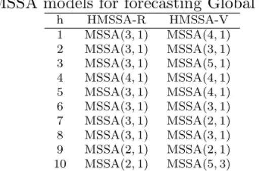
Finally, in Table 1 we present the MSSA models for obtaining the forecasts for GT at each horizon.
Table 1: MSSA models for forecasting Global Temperature.
h HMSSA-R HMSSA-V 1 MSSA(3,1) MSSA(4,1) 2 MSSA(3,1) MSSA(3,1) 3 MSSA(3,1) MSSA(5,1) 4 MSSA(4,1) MSSA(4,1) 5 MSSA(3,1) MSSA(4,1) 6 MSSA(3,1) MSSA(3,1) 7 MSSA(3,1) MSSA(2,1) 8 MSSA(3,1) MSSA(3,1) 9 MSSA(2,1) MSSA(2,1) 10 MSSA(2,1) MSSA(5,3)
Note: Shown here in brackets are the combinations ofLandras MSSA(L, r).
4
Data and Metrics
4.1 Data
The data we investigate here consists of two variables, namely the global temperature anomaly (GT) and global carbon dioxide (CO2) emissions, and spans the annual period of 1880-2012,
with the start and end of the period being purely driven by the availability of data. GT measures the difference between a reference long-term average value (which happens to be 1951-1980) and the actual value. The calculation of GT is in itself a complex process adjusting for aspects such as, though not limited to, unequal distance between measuring stations, difference due to the richly observed northern hemisphere versus the poorly observed southern hemisphere, ocean
versus terrestrial measurements, polar regions, into one representative number for the whole earth (Hansen et al., 2010). Similarly global CO2 is estimated from energy statistics published
by the United Nations (2014) involving a complex system comprising of, again not limited to, questionnaires, official statistics and other supplementary information (Boden et al., 1995). The
GT were obtained from the National Aeronautics and Space Administrations (NASA) and the
Goddard Institute for Studies (GISS).8 The data on CO2 was obtained from theCarbon Dioxide Information Analysis Centre 9 and is measured in thousand metric tons of carbon. While GT
remains untransformed in our analysis, we use the natural logarithm of CO2 emissions. The
log transformation allows us to make the highly skewed distribution of CO2 less skewed, which
in turn, is valuable both for making patterns in the data more interpretable and for helping to meet the assumptions of inferential statistics.
4.2 Forecasting Exercise
We separate the entire data period into an initial in-sample period spanning 1880-1906, and an out-of-sample period of 1907-2012. Note that, since we use a recursive estimation for the models (barring RW and SSA), we have an expanding in-sample period, while producing the out-of-sample forecasts for the various horizons. This separation of the period was determined by the Bai and Perron (2003) tests of multiple structural breaks applied to the global temperatures equation of the VAR model, which, in turn, detected the following break dates: 1907, 1945, 1974, 1992, and 2004. Since our linear models are estimated recursively over the out-of-sample period in which all the break dates fall, this separation of the period is ideal as it helps us to accommodate changes in the parameter estimates of the model in the out-of-sample period. In other words, if we would have a split in the initial in-sample and out-of-sample periods different from the one based on the structural break tests, with some of the breaks in the initial in-sample period, the linear models would be misspecified. This is because, the linear models would not be capturing the change in the response of GT to CO2 emissions that took place due to breaks
in the initial in-sample. This way, we aim to make the comparison between linear and nonlinear models fair, by ensuring that the superior predictability of the nonlinear models, if and when it exists, is not because of misspecification due to regime changes but due to the inherent nonlinear relationship of GT with CO2.10 Finally, we produce one- to ten-year-ahead forecasts based on
this recursive estimation scheme to forecast in the short- and long-term horizon. Except for the MSSA models where the initial model remains constant and the data is updated, all other models update the data and re-estimate model parameters each time a new observation is introduced. Accordingly, we generate forecasts at each horizon such that we have n−h+ 1 observations where n= 106 andh refers to the horizon of interest.
4.3 Descriptive Statistics
Table 2 summarises the descriptive statistics for the entire GT data set, and the in-sample and out-of-sample periods separately. This analysis uncovers some interesting insights relating to the series. Firstly, the structure of the series overall and out-of-sample appears to be closely associated as expected (given the large out-of-sample forecasting period). Both these series are
8The data is available for download from: http://data.giss.nasa.gov/gistemp/.
9The data is available for download from: http://cdiac.ornl.gov/trends/emis/treglob
2013.html. 10
Given that, the structural break test is performed on the full-sample of the data, which in turn, is not available to a forecaster while making a forecast, we reconducted our analysis using an initial in-sample period of 1880-1946 i.e., essentially a 50 percent split of the data. Our revised analyses, which are available upon request, produced qualitatively similar results.
skewed and report an almost identical interquartile range (IQR), and the out-of-sample data captures the overall minimum and maximum GT values. In comparison, the initial in-sample series captures a period where the GT values are negative and normally distributed.
Table 2: Descriptive statistics for GT.
Min Max Mean Med. SD IQR SW(p)
Overall (1880-2012) -47 66 -1.47 -7 28.96 35 <0.01
In-Sample (1880-1906) -44 -10 -25.44 -25 8.09 12.5 0.95*
Out-of-Sample (1907-2012) -47 66 4.63 2.50 29.20 36.75 <0.01 Note:∗indicates data is normally distributed based on the Shapiro-Wilk (SW) test atp=0.01.
4.4 Metrics
To evaluate the 12 competing models, we use the popular Root Mean Squared Error (RMSE) loss function and the direction of change (DC) criteria for comparing their forecasting perfor-mances. All outcomes relating to forecast accuracy are tested for statistical significance using the Kolmogorov-Smirnov Predictive Accuracy (KSPA) test (Hassani and Silva, 2015), whilst the DC results are tested for statistical significance using a Student’s t-test.
Root Mean Squared Error (RMSE)
The RMSE is now a standard quantitative technique for evaluating forecasting accuracy of alternate models. It is also popular as one of the most frequently cited measures in forecasting literature (see, for example, Zhang et al. (1998) and Hassani et al. (2015b)). In this paper we consider both the RMSE and Ratio of the RMSE (RRMSE). Here, in order to save space we present only the RRMSE.
RRMSE = PN i=1( ˆYT+h,i−YT+h,i)2 PN i=1( ˜YT+h,i−YT+h,i)2 !1/2 ,
where ˆYT+h represents the h-step ahead forecast obtained by the benchmark model, ˜YT+h
rep-resents the h-step ahead forecast obtained by a competing model, and N is the number of
forecasts. If RRMSE < 1 then the benchmark model outperforms the competing model by
1-RRMSE percent.
Direction of Change (DC)
The DC metric is an equally important measure as the RMSE because it is able to show whether the forecast is correctly predicting the actual direction of change. A model is said to have a better DC prediction than a random walk if it records a DC greater than 50% (Altavilla and de Grauwe, 2010). The DC calculation is presented below and in doing so we mainly follow Hassani et al., (2013a).
Consider a univariate time series YT. Let ZY i take the value 1 if the forecast correctly
predicts the direction of change and 0 otherwise. Then ¯ZX =PNi=1ZY i/N shows the proportion
5
Empirical Results
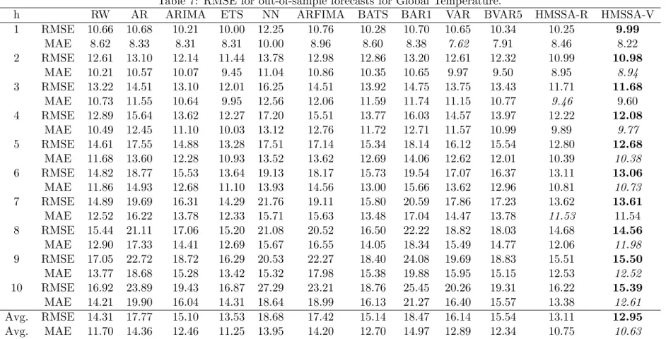
Forecasting results covering all horizons from 1-10 can be found in Tables 7 and 8. The presenta-tion of the results which considers both short and long term forecasts of GT enables stakeholders to select the best model at each forecast horizon of interest. Here in Tables 3 and 4, we present a summarised version of the out-of-sample forecasting results for GT which considers horizons 1, 5, and 10, and thereby represents the short, medium and long term forecasts. We initially dis-cuss the overall results. The first observation is that the HMSSA-V model can provide the best forecast for GT across all horizons. Also, it is important to note that the two MSSA techniques with their various fitted models succeed in reporting the lowest RMSE and MAE in comparison to all models evaluated here, across all horizons. As such, in relation to all models considered in this study, we are able to identify clearly that MSSA has the potential to provide the most accurate forecasts for GT when CO2 is used as auxiliary information. Secondly, given that these
superior MSSA results have been attained by using CO2 as an indicator variable, we are able to
conclude that CO2 can indeed help in predicting GT. If one is interested in a single model for
obtaining the best possible forecasts for GT, then based on the average lowest RMSE and MAE we can propose that specifically the HMSSA-V technique, as used in this study, is best for this purpose.
The results also enable a more detailed analysis and differentiation between univariate and multivariate models. In terms of the univariate models we see that across all horizons, ETS forecasts are best for GT (Table 7). Interestingly as well, on most occasions the RW forecasts are seen outperforming the univariate models (except ETS), and also outperforming the multivariate
BVAR5 and VAR forecasts with the exception of h = 1 step ahead results from VAR and
BVAR5 models. Another point to note is that forecasts for GT from the univariate BAR1 model is almost as bad as the worst performing NN model according to the average RMSE and MAE criteria. Furthermore, as both univariate and multivariate models are considered in this study, practitioners also have the option of selecting the best univariate or multivariate model for forecasting GT at a particular horizon of interest.
The RMSE and MAE results reported in Table 7 clearly indicates how the forecasting accu-racy of all models deteriorates as the forecasting horizon expands from 1-step ahead to 10-steps ahead. A closer look at these results show that ETS and HMSSA models incur a deterioration in accuracy levels at a comparatively slower rate than rest of the models. This in turn indicates that the univariate ETS model is performing considerably well in relation to other univariate models considered here, and also that the MSSA models are performing better than all other models in terms of the RMSE criteria.
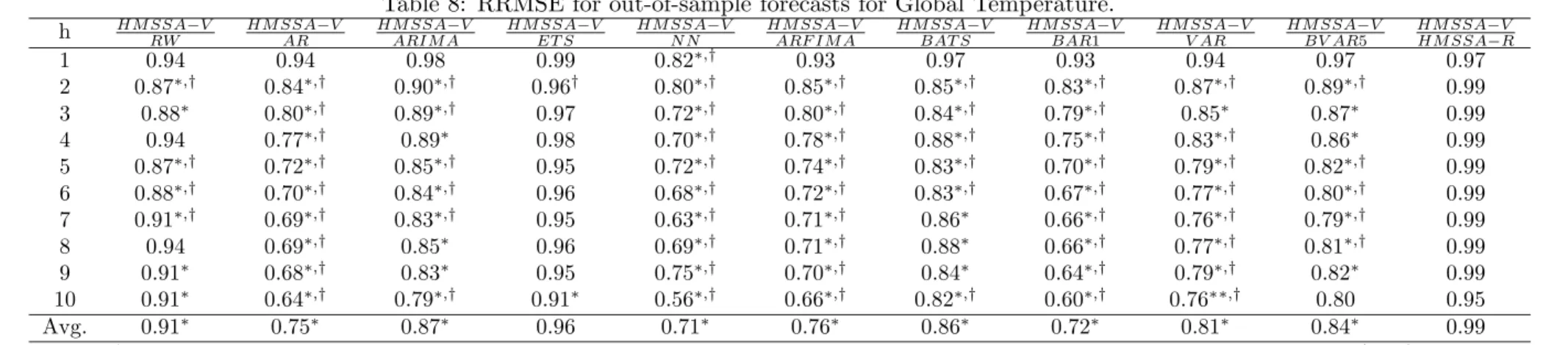
In Table 4 we consider HMSSA-V as a benchmark model and present the RRMSE results for GT forecasts for horizons 1, 5, and 10 steps-ahead with Table 8 reporting all results. The choice of HMSSA-V as a benchmark model was influenced by the fact that the HMSSA-V model reports the lowest RMSE and lowest average MAE across all ten forecasting horizons. Here we exploit the two-sided HS test (Hassani and Silva, 2015) and the modified Diebold-Mariano test to find statistically significant differences between forecasts across all 10 forecasting horizons. Evidence from the two-sided KSPA test (results indicated on the ‘Avg.’ row in Table 4) suggests that on average, across all 10 horizons, the only instance in which HMSSA-V fails to produce a forecast that is not significantly better than another model’s forecast is in comparison to HMSSA-R and ETS forecasts at a 90% confidence level. This provides added justification for selecting the HMSSA-V model proposed in this study as a benchmark for forecasting GT. At the same time, it also shows the power of the ETS model for those wishing to rely on a univariate forecasting approach when modelling GT.
The RRMSE results in Table 4 are further tested for statistical significance via the two-sided KSPA test which seeks to ascertain the existence of a statistically significant difference between the distributions of two forecast errors. Leaving aside the HMMSA-R and HMSSA-V models which do not report any statistically significant differences between forecast errors at the
90% confidence level, we can conclude that beyond h = 1, the HMSSA-V forecasts are indeed
significantly better than all other competing forecasts on most instances (with the exception of
ETS). Interestingly, HMSSA-V forecasts only outperformed ETS at h = 2 and h = 10 steps
ahead. Also, we failed to find evidence of statistically significant differences between forecasts
of HMSSA-V and RW models at h = 1, 4, and 8 steps ahead. The beauty of the RRMSE
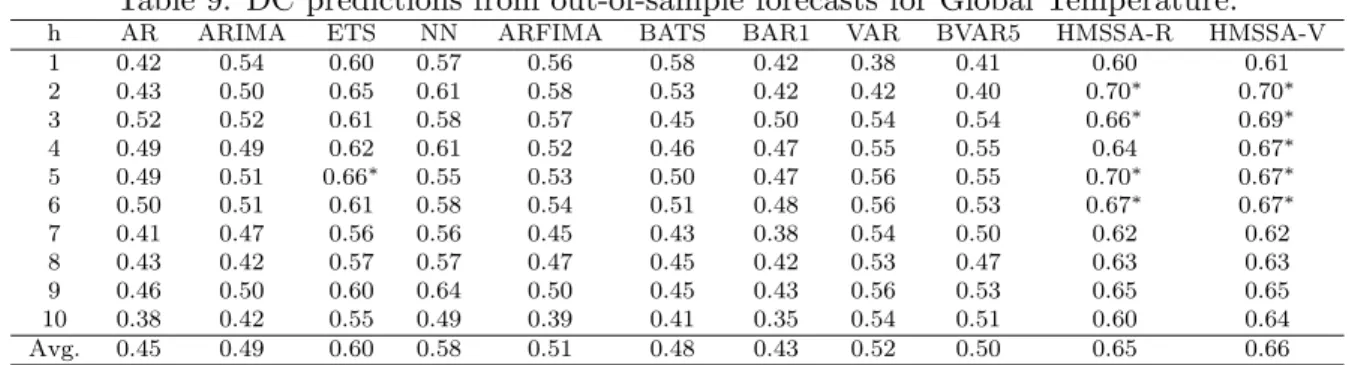
criterion is that it enables us to further quantify the performance of a given forecasting model and show by what percentage it outperforms forecasts from another model. Accordingly, based on the RRMSE we are able to conclude that on average, across all ten horizons, the HMSSA-V forecasts are better in the range of 1% (relative to the HMSSA-R) and 29% (relative to the NN). Presented in Table 5 (summarized output) and Table 9 (all output) are the DC prediction results from the GT forecasts. It is important to evaluate the accuracy of a model in its ability to correctly predict the actual direction of change in the time series.11 The DC results indicate that
on average the univariate BAR1 model is worst in predicting the actual direction of change in GT. If we consider only the univariate models, then the AR model has the worst DC prediction whilst the ETS model reports the best. In terms of multivariate models, the MSSA models report the best DC predictions on average and are almost identical. However, if one was to suggest a single model with the best average DC prediction then it would be the HMSSA-V model with an average accuracy of 66%. The inclusion of the DC results at each horizon enables practitioners to select the best model for a particular forecasting horizon not only based on the RMSE criterion but also based on its ability at providing a good DC prediction for GT. In line with good statistical practice we test all DC predictions for statistical significance using the Student’st-test as in Hassani et al. (2009). Accordingly, we see that the DC predictions reported for AR, ARIMA, ARFIMA, NN, BATS, BAR1, VAR, and BVAR5 models at all horizons are
likely to be a result of chance occurrences. However, the DC prediction for ETS at h = 5
steps ahead is found to be statistically significant whilst half of the DC predictions from the HMSSA-V model report statistically significant outcomes. As such, we are able to conclude with 90% confidence that the HMSSA-V DC predictions are significantly greater than 50% across forecasting horizons 2-6.
11Note that it is not possible to calculate the DC metric for RW forecasts as it results in the DC statistic going to infinity.
Table 3: RMSE for out-of-sample forecasts for Global Temperature.
h RW AR ARIMA ETS NN ARFIMA BATS BAR1 VAR BVAR5 HMSSA-R HMSSA-V
1 RMSE 10.66 10.68 10.21 10.00 12.25 10.76 10.28 10.70 10.65 10.34 10.25 9.99 MAE 8.62 8.33 8.31 8.31 10.00 8.96 8.60 8.38 7.62 7.91 8.46 8.22 5 RMSE 14.61 17.55 14.88 13.28 17.51 17.14 15.34 18.14 16.12 15.54 12.80 12.68 MAE 11.68 13.60 12.28 10.93 13.52 13.62 12.69 14.06 12.62 12.01 10.39 10.38 10 RMSE 16.92 23.89 19.43 16.87 27.29 23.21 18.76 25.45 20.26 19.31 16.22 15.39 MAE 14.21 19.90 16.04 14.31 18.64 18.99 16.13 21.27 16.40 15.57 13.38 12.61
Note: Shown in bold font is the model reporting the lowest RMSE. The model reporting the lowest MAE is italicised. The multivariate models use CO2 at lag 2.
Table 4: RRMSE for out-of-sample forecasts for Global Temperature.
h HM SSA−V RW HM SSA−V AR HM SSA−V ARIM A HM SSA−V ET S HM SSA−V N N HM SSA−V ARF IM A HM SSA−V BAT S HM SSA−V BAR1 HM SSA−V V AR HM SSA−V BV AR5 HM SSA−V HM SSA−R 1 0.94 0.94 0.98 0.99 0.82∗,† 0.93 0.97 0.93 0.94 0.97 0.97 5 0.87∗,† 0.72∗,† 0.85∗,† 0.95 0.72∗,† 0.74∗,† 0.83∗,† 0.70∗,† 0.79∗,† 0.82∗,† 0.99 10 0.91∗ 0.64∗,† 0.79∗,† 0.91∗ 0.56∗,† 0.66∗,† 0.82∗,† 0.60∗,† 0.76∗,† 0.80 0.95 Avg. 0.91∗ 0.75∗ 0.87∗ 0.96 0.71∗ 0.76∗ 0.86∗ 0.72∗ 0.81∗ 0.84∗ 0.99
Note: ∗indicates a statistically significant difference between the distribution of forecasts based on the two-sided KSPA test in Hassani and Silva (2015) at
p= 0.10. †indicates the existence of a statistically significant difference between the forecasts based on the modified Diebold-Mariano test in Harvey et al. (1997).
Table 5: DC predictions from out-of-sample forecasts for Global Temperature.
h AR ARIMA ETS NN ARFIMA BATS BAR1 VAR BVAR5 HMSSA-R HMSSA-V 1 0.42 0.54 0.60 0.57 0.56 0.58 0.42 0.38 0.41 0.60 0.61 5 0.49 0.51 0.66∗ 0.55 0.53 0.50 0.47 0.56 0.55 0.70∗ 0.67∗
10 0.38 0.42 0.55 0.49 0.39 0.41 0.35 0.54 0.51 0.60 0.64 Avg. 0.45 0.49 0.60 0.58 0.51 0.48 0.43 0.52 0.50 0.65 0.66
Note: ∗indicates the DC prediction is statistically significant based on a Student’sttest atp= 0.05.
5.1 Robustness Analysis
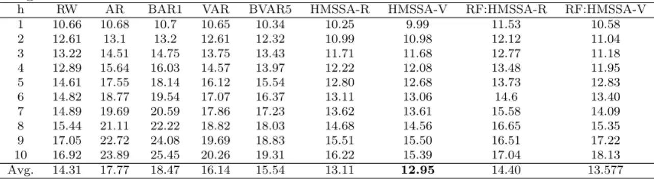
Though we followed the works of Fildes and Kourentzes (2011), and McMillan and Wohar (2013) in using CO2 emissions as a predictor variable for GT, based on the suggestion of the Editor, we
also evaluated the performance of our SSA models using radiative forcing instead of CO2. Note,
radiative forcing is defined as the difference of insolation (sunlight) absorbed by the Earth and energy radiated back to space. We observed that just like the MSSA models with CO2, the same
models with radiative forcing outperformed the univariate and multivariate linear models and the neural network model. However, the HMSSA-V model based on total radiative forcing, could
only outperform the HMSSA-R and HMSSA-V based on CO2emissions at horizons of three- and
four-year-ahead. Also, on average, the HMSSA-R and HMSSA-V using CO2emissions continued
to perform the best. A selection of these results are reported via Table 6 for the benefit of the reader.
Table 6: RMSE results from out-of-sample forecasts for Global Temperature using Radiative Forcing.
h RW AR BAR1 VAR BVAR5 HMSSA-R HMSSA-V RF:HMSSA-R RF:HMSSA-V 1 10.66 10.68 10.7 10.65 10.34 10.25 9.99 11.53 10.58 2 12.61 13.1 13.2 12.61 12.32 10.99 10.98 12.12 11.04 3 13.22 14.51 14.75 13.75 13.43 11.71 11.68 12.77 11.18 4 12.89 15.64 16.03 14.57 13.97 12.22 12.08 13.48 11.95 5 14.61 17.55 18.14 16.12 15.54 12.80 12.68 13.73 12.83 6 14.82 18.77 19.54 17.07 16.37 13.11 13.06 14.6 13.40 7 14.89 19.69 20.59 17.86 17.23 13.62 13.61 15.58 14.09 8 15.44 21.11 22.22 18.82 18.03 14.68 14.56 16.65 15.35 9 17.05 22.72 24.08 19.69 18.83 15.51 15.50 16.51 17.22 10 16.92 23.89 25.45 20.26 19.31 16.22 15.39 17.04 18.13 Avg. 14.31 17.77 18.47 16.14 15.54 13.11 12.95 14.40 13.577
6
Discussion
The discussion begins with a graphical illustration of the the best out-of-sample forecasts for GT in the very short run (h= 1) and the very long run (h= 10) as shown via Figure 2. All forecasts shown are from the HMSSA-V model. Interestingly, the forecasts from the other models showed clear signs of difficulties in modelling and providing an accurate forecast for GT amidst the variation visible in the series, and in most cases the competing models were seen picking up the variations too late in time and reflecting on the comparatively poor DC predictions reported in Table 5. The use of MSSA models enabled to overcome the issues pertaining to modelling the volatility in GT and provide forecasts which are comparatively more accurate and reliable for decision making.
h=1
Time
Global T
emper
ature Anomaly (GT) in Celsius
1920 1960 2000 −40 −20 0 20 40 60 GT HMSSA−V h=10 Time Global T emper
ature Anomaly (GT) in Celsius
1920 1940 1960 1980 2000 −40 −20 0 20 40 60 80 GT HMSSA−V
Figure 2: Out-of-sample MSSA forecasts for GT.
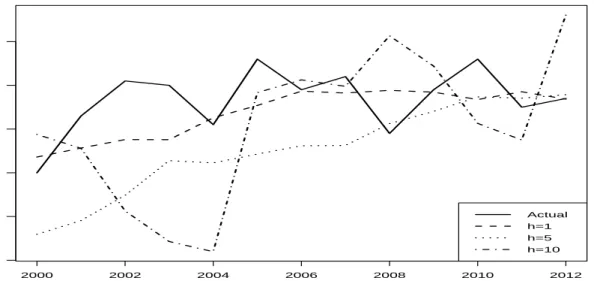
However, as evident via Figure 2, even the best forecasts appear to have difficulty in capturing the levelling which occurs post 2000 until recently. As such, it is pertinent to briefly comment on this. For this purpose, shown via Figure 3 are the best performing one, five, and ten-steps ahead forecasts from 2000 onwards based on the lowest RMSE criteria. All forecasts appearing here are from the HMSSA-V model. Notice how some of the forecasts appear to fluctuate whilst the others are represented as comparatively smoother lines. There are two possible explanations for this. Firstly, MSSA is sensitive to the choice of window length Land the number of eigenvalues
r, and the automated MSSA algorithm introduced in this paper is programmed to find the best possible forecast by minimising a loss function. Therefore, instead of seeking out components which will capture most of the fluctuations, more weighting is given to the forecast line which can reduce the error. Secondly, the MSSA algorithm does not update and fit a new model to the data each time a new observation is introduced. Whilst this approach does provide more stability to the forecasting model, it does however make it difficult for the model to ensure the levelling which occurs towards the end of the out-of-sample period is accurately captured. Yet, it is noteworthy that in comparison to the other models which are all recursive, these MSSA forecasts with a fixed model fitted at the training stage is able to outperform the rest. Given the non-recursive nature of the MSSA forecasts, as the horizon increases beyond 1-step ahead, we notice a deterioration in the forecast accuracy (it still deteriorates at a lower rate than the recursive models). It would be interesting to see whether programming recursive MSSA models can enable MSSA to capture the levelling post 2000 more accurately.
Time
Global T
emper
ature Anomaly (GT) in Celsius
2000 2002 2004 2006 2008 2010 2012 20 30 40 50 60 70 Actual h=1 h=5 h=10
Figure 3: The best out-of-sample forecasts (HMSSA-V model) post 2000 at selected horizons. Given that GT data is now available till 2017, below, we also show the ex ante forecasts from the best MSSA models using CO2and total radiative forcing (TRF) as auxiliary information. As
expected, based on the forecasting exercise carried out in this study, we see that the HMSSA-V model using CO2 as auxiliary information performs the best in tracking more closely the trend
of GT.
Time
Global T
emper
ature Anomaly (GT) in Celsius
2013 2014 2015 2016 2017
60
70
80
90
100
Actual GT HMSSA−R(TRF) HMSSA−V (TRF) HMSSA−R(CO2) HMSSA−V(CO2)Figure 4: The best MSSA forecasts for GT 2013-2017.
At this stage, it is important to compare our results with the existing evidence of predictabil-ity of GT emanating from CO2 emissions. As discussed in the introduction, available studies
two, with bulk of the papers using climate models. Just as in McMillan and Wohar (2013), we find no evidence of the ability of CO2 emissions in predicting GT based on linear models. This
weak evidence is not surprising given that the Brock et al., (BDS, 1996) test indicated strong evidence of nonlinearity in the relationship between the two variables.12 However, unlike in
Fildes and Kourentzes (2011) to certain extent, we found that, even though nonlinearity exists, a NN model cannot seem to capture this underlying nonlinearity well enough, as is indicated in its poor forecasting performance. The superiority of the SSA models in forecasting however, tend to suggest that these models are able to better capture this unknown nonlinear relationship via a nonparametric formulation.13
7
Conclusions
The two popular and passionate debates about climate change are (i) Is it possible to predict global temperature anomaly (GT) reliably?; and (ii) Is there definitive causal evidence of (an-thropometric) CO2being the driver of GT? This paper is an exercise to contribute to this debate
by providing objective analyses of relevant data using an ensemble comprising of 12 parametric and nonparametric out-of-sample forecasting techniques using only GT data (univariate), as well as using both GT and CO2 data (multivariate). The significance of this paper lies in that, using
the well established datasets we have identified the ‘best’ model, from 12 candidate models, for forecasting GT both in the short- and long-term horizons. Specifically, our results have identified that the Horizontal Multivariate Singular Spectral Analysis (HMSSA) models (both Recurrent (-R) and Vector (-V)) consistently outperform the other competing models in a statistically significant fashion. Further, from the performance of the HMSSA-R model, we have conclusive evidence that CO2 can predict GT. We also evaluated the models in their ability to predict the
direction of change (DC) for the GT forecasts. Although in the univariate setup the exponential smoothing (ETS) model performs best in forecasting DC followed by the HMSSA models, in the multivariate setup, the HMSSA models once again score best when evaluated using the metrics considered. Thus, from our investigation and from the analyses of the findings, if we have to recommenda model for forecasting GT, HMSSA-R is a clear winner. Our results also highlight the superiority of the nonparametric approach of the SSA, which in turn, allows us to handle any statistical process: linear or nonlinear, stationary or non-stationary, Gaussian or non-Gaussian. Hence, from the perspective of a climate modeller relying on AOGCMs, it would make sense to compare the ex ante forecasts (i.e., future path) of GT generated from the SSA model with that from the AOGCMs. In this regard, as part of future analysis, it would be interesting to go back and compare the future paths generated in historical reports of IPCC on GT, with that generated from our SSA model. Using historical comparison will allow us to determine how far or close the paths generated by the climate models and that by time series models match up with what actually materialized in terms of global temperature levels. Also note, using the SSA model, given that it is based on bootsrapping, we will be able to generate interval and density forecasts for global temperatures, thus allowing us to determine the uncertainty associated with such forecasts.
Though the objective of this paper was to pursue a forecasting exercise to determine whether
CO2 emissions can predict the future movements in GT, using a large number of linear and
nonlinear models, our results can be utilized to draw important policy conclusions as well. We show that it is important to model nonlinearity into the relationship between GT and CO2,
12Complete details of these results are available upon request from the authors.
13This line of thinking is vindicated by the superior fit of the SSA approach relative to the NN method. Complete details of the goodness-of-fit results are available upon request from the authors.
otherwise, the latter does not seem to contain any predictive information about the future paths of GT. Once this is done, we find strong evidence of the role of CO2 in increasing GT, i.e., we
show that continued CO2 emissions will cause further warming.14
Our findings also open up several avenues for future research. It would be interesting to analyze the emissions from various countries including the top emitters, to determine which countries can predict global temperatures the best, and also to find out whether the top emitters can predict global temperatures better than world emissions. The findings from such analysis can help design better policies. Also, it is important to point out that, while we only concentrate on CO2 emissions in this paper, there is also a large literature that has related global temperatures
to sunspots, but primarily based on in-sample analysis (see Hassani et al., (2016) for a detailed review). Given this, in the future it would be interesting to extend this literature to out-of-sample forecasting, and also include sunspot along with CO2 emissions to check the robustness
of our results.
14Based on the suggestion of an anonymous referee, we estimated a time-varying model of cointegration as outlined in Bierens and Martins (2010). Based on this framework, we observed that the response of GT to CO2 has steadily decreased post World War II, with the average impact suggesting that one unit increase in CO2 would increase GT by 0.0486 unit. Complete details of these results are available upon request from the authors. As discussed in the Fifth Climate Change Synthesis Report of the IPCC (2014), continuous global warming will have long-lasting changes in all components of the climate system, increasing the likelihood of severe, pervasive and irreversible impacts for both people and ecosystems. In addition, climate change will amplify existing risks and create new risks for natural and human systems; with risks being higher for vulnerable communities around the world, resulting in an unequal society, and hamper socio-economic development. Understandably, limiting climate change would require not only substantial and sustained reductions in CO2 emissions (mitigation), but also adaptation, to limit negative climate change impacts.
References
Altavilla, C. and De Grauwe, P. (2010). Forecasting and combining competing models of ex-change rate determination,Applied Economics, 42, 3455–3480.
Bai J., and Perron P. (2003). Computation and Analysis of Multiple Structural Change Models.
Journal of Applied Econometrics, 18, 1–22.
Beenstock, M., Reingerwertz, Y., and Paldor, N. (2016). Testing the Historic Tracking of Climate Models. International Journal of Forecasting, 32(4), 12341246.
Beneki, C., Eeckels, B., and Leon, C. (2012). Signal extraction and forecasting of the UK tourism income time series: a Singular Spectrum Analysis approach. Journal of Forecasting, 31, 391–400.
Bierens, H.J. and Martins, L.F. (2010). Time Varying Cointegration.Econometric Theory 26, 14531490.
Boden, T.A., G. Marland, and R. J. Andres. (1995). Estimates of global, regional, and national annual CO2 emissions from fossil-fuel burning, hydraulic cement production, and gas flaring:
1950-1992.ORNL/CDIAC-90, NDP-30/R6. Oak Ridge National Laboratory, U.S. Department
of Energy, Oak Ridge, Tennessee.
Brock, W., Dechert, D., Scheinkman, J. and LeBaron, B. (1996). A Test for Independence Based on the Correlation Dimension.Econometric Reviews, 15, 197235.
Campbell, J.Y. (2008). Viewpoint: Estimating the Equity Premium. Canadian Journal of
Economics, 41, 1-21.
De Livera, A. M., Hyndman, R. J., and Snyder, R. D. (2011), Forecasting time series with complex seasonal patterns using exponential smoothing. Journal of the American Statistical Association, 106, 1513–1527.
Dergiades, T., Kaufmann, R., Panagiotidis, T. (2016) Long-Run Changes in Radiative Forcing and Surface Temperature: The Effect of Human Activity over the Last Five Centuries.Journal of Environmental Economics and Management, 76, 67–85.
Fildes, R., and Kourentzes, N. (2011). Validation and forecasting accuracy in models of climate change.International Journal of Forecasting, 27, 968-995.
Ghil, M., Allen, M. R., Dettinger, M. D., Ide, K., Kondrashov, D., Mann, M. E., Robertson, A. W., Saunders, A., Tian, Y., Varadi, F., and Yiou, P. (2002). Advanced spectral methods for climatic time series.Reviews of Geophysics, 40, 1–41.
Ghil, M., and Vautard, R. (1991). Interdecadal oscillations and the warming trend in global temperature time series.Nature, 350, 324–327.
Green, K. C., and Armstrong, J. S. (2007). Global warming: forecasts by scientists versus scientific forecasts.Energy and Environment, 18, 997-1021.
Groth, A., and Ghil, M. (2012). Multivariate singular spectrum analysis and the road to phase synchronization. Physical Review E, 84, 036206.
Gupta, R., and Kabundi, A. (2010). Forecasting macroeconomic variables in a small open economy: a comparison between small- and large-scale models, Journal of Forecasting, 29(1-2), 168-185.
Gupta, R., and Kabundi, A. (2011). A large factor model for forecasting macroeconomic vari-ables in South Africa,International Journal of Forecasting, 27(4), 1076-1088.
Gupta, R., and Kabundi, A., Miller, S.M., and Uwilingiye, J. (2014). Using large data sets to forecast sectoral employment,Statistical Methods & Applications 23(2), 229-264.
Hansen, P. R., Peter, R., Lunde, A., Nason, J. M. and James, M. (2011). The Model Confidence Set.Econometrica, 79, 453–497.
Hansen, J. E., Sato, M., Ruedy, R., Lacis, A., and Glascoe, J. (1998). Global climate data and models: A reconciliation.Science, 281, 930932.
Hansen, J., Ruedy, R., Sato, M., and Lo, K. (2010) Global surface temperature change. Rev Geophys 48, RG4004, 1-29.
Harvey, D. I., Leybourne, S. J., and Newbold, P. (1997). Testing the equality of prediction mean squared errors.International Journal of Forecasting, 13, 281-291.
Haslett, J., and Raftery, A. E. (1989). Space-time Modelling with Long-memory Dependence: Assessing Ireland’s Wind Power Resource (with discussion),Applied Statistics, 38, 1–50.
Hassani, H. (2007). Singular Spectrum Analysis: Methodology and Comparison. Journal of
Data Science,5(2), pp. 239-257.
Hassani, H., Heravi, H., and Zhigljavsky, A. (2009). Forecasting European industrial production with Singular Spectrum Analysis.International Journal of Forecasting, 25, 103–118.
Hassani, H., Heravi, H., and Zhigljavsky, A. (2013a). Forecasting UK industrial production with multivariate singular spectrum analysis.Journal of Forecasting, 32, 395–408.
Hassani, H., Huang, X., Gupta, R., and Ghodsi, M. (2016). Does sunspot numbers cause global temperatures? A reconsideration using non-parametric causality tests. Physica A: Statistical Mechanics and its Applications, 460(C), 54-65.
Hassani, H. and Mahmoudvand, R. (2013). Multivariate Singular Spectrum Analysis: A general view and new vector forecasting approach.International Journal of Energy and Statistics, 1, 55–83.
Hassani, H., and Silva, E. S. (2015). A Kolmogorov-Smirnov Based Test for Comparing the Predictive Accuracy of Two Sets of Forecasts. Econometrics, 3, 590–609.
Hassani, H., Silva, E. S., Gupta, R., and Segnon, M. K. (2015b). Forecasting the price of gold.
Applied Economics, 47, 4141–4152.
Hassani, H., Soofi, A. S., and Zhigljavsky, A. A. (2010c). Predicting daily exchange rate with singular spectrum analysis.Nonlinear Analysis: Real World Applications, 11, 2023–2034. Hassani, H., Soofi, A. S., and Zhigljavsky, A. (2013b). Predicting inflation dynamics with singular spectrum analysis.Journal of the Royal Statistical Society A, 176, 743–760.
Hassani, H., Webster, A., Silva, E. S., and Heravi, S. (2015a). Forecasting U.S. Tourist arrivals using optimal Singular Spectrum Analysis.Tourism Management, 46, 322–335.
Hyndman, R. J. (2006). Another look at forecast-accuracy metrics for intermittent demand.
Foresight, 4, 43–46.
Hyndman, R. J., and Athanasopoulos G. (2013).Forecasting: principles and practice. OTexts: Australia. OTexts.com/fpp.
Hyndman, R. J., and Khandakar, Y. (2008). Automatic time series forecasting: The forecast Package for R.Journal of Statistical Software, 27, 1–22.
Hyndman, R. J., Athanasopoulos, G., Razbash, S., Schmidt, D., Zhou, Z., Khan, Y., & Bergmeir, C. (2013). Package forecast: Forecasting functions for time series and linear models.
Available via: http://cran.r-project.org/web/packages/forecast/forecast.pdf.
[Ac-cessed: 08 August 2015]
Kaufmann, R. K., and Stern, D. I. (2004). A statistical evaluation of atmosphere-ocean general circulation models: complexity v simplicity. Rensselaer Working Papers in Economics, No. 0411.
Khandekar, M.L., Murty, T.S., and Chittibabu, P. (2005) The global warming debate: a review of the state of science.Pure Appl Geophys, 162, 15571586.
Kwiatkowski, D., Phillips, P. C. B., Schmidt, P., and Shin, Y. (1992). Testing the null hy-pothesis of stationarity against the alternative of a unit root. Journal of Econometrics, 54, 159–178.
Lisi, F., and Medio, A. (1997). Is a random walk the best exchange rate predictor? International Journal of Forecasting, 13, 255–267.
Litterman, R. B. (1981). A Bayesian Procedure for Forecasting with Vector Autoregressions.
Working Paper, Federal Reserve Bank of Minneapolis.
Litterman, R. B. (1986). Forecasting with Bayesian Vector Autoregressions: Five Years of Experience.Journal of Business and Economic Statistics, 4, 25–38.
Makridakis, S. G., Wheelwright, S. C., and Hyndman, R. J. (1998) Forecasting: Methods and Applications. 3rd edn, Wiley: New York.
McMillan, D.G., Wohar, M. E. (2013). The relationship between temperature and CO2
emis-sions: evidence from a short and very long dataset.Applied Economics, 45, 3683-3690.
McSharry, P.E. (2011). Validation and forecasting accuracy in models of climate change: Com-ments.International Journal of Forecasting, 27, 996999.
Oropeza, V., and Sachchi, M. (2011). Simultaneous seismic data denoising and reconstruction via multichannel singular spectrum analysis.Geophysics, 76, V25–V32.
Patterson, K., Hassani, H., Heravi, S., and Zhigljavsky, A. (2011). Multivariate singular spec-trum analysis for forecasting revisions to real-time data. Journal of Applied Statistics, 38, 2183–2211.