of Supervised Learning Methods
for Malware Analysis
Michał Kruczkowski
1,2and Ewa Niewiadomska-Szynkiewicz
1,3 1Research and Academic Computer Network NASK, Warsaw, Poland 2
Institute of Computer Science, Polish Academy of Sciences, Warsaw, Poland 3
Institute of Control and Computation Engineering, Warsaw University of Technology, Warsaw, Poland
Abstract—Malware is a software designed to disrupt or even damage computer system or do other unwanted actions. Nowadays, malware is a common threat of the World Wide Web. Anti-malware protection and intrusion detection can be significantly supported by a comprehensive and extensive analysis of data on the Web. The aim of such analysis is a classification of the collected data into two sets, i.e., nor-mal and nor-malicious data. In this paper the authors investigate the use of three supervised learning methods for data min-ing to support the malware detection. The results of applica-tions of Support Vector Machine, Naive Bayes andk-Nearest Neighbors techniques to classification of the data taken from devices located in many units, organizations and monitoring systems serviced by CERT Poland are described. The perfor-mance of all methods is compared and discussed. The results of performed experiments show that the supervised learning algorithms method can be successfully used to computer data analysis, and can support computer emergency response teams in threats detection.
Keywords—data classification, k-Nearest Neighbors, malware analysis, Naive Bayes, Support Vector Machine.
1. Introduction
Malicious software (malware) is software designed to dis-rupt or damage computer system, gain access to users or gather sensitive information. Malicious programs can be classified into worms, viruses, trojans, spywares, etc. In recent years numerous attacks have threaten the ability and operation of the Internet. Therefore, mechanisms for suc-cessive detection of malicious software are crucial compo-nents of network security systems. In this paper the use of selected data mining techniques to malware analysis is investigated. Comprehensive and extensive analysis of data on the Web can significantly improve the results of malware detection. A large number of learning based methods have been developed over the past decades and used to com-plex data analysis. The taxonomy and survey are provided in [1]. Recently, a class of supervised learning methods has emerged as powerful techniques for heterogenous data analysis and classification. It is obvious that most data on the World Wide Web is heterogeneous, unstructured, and often incomplete. Therefore, in presented research the
au-thors focus on the application of the supervised methods to malware detection.
The goal is to detect malware based on classification of data taken from various computer networks that belong to various users and organizations. The objective is to classify a given program on the Web into a malware or a clean class. Hence, a problem of two-class pattern classification is considered.
The problem of identifying to which set of categories a new observation (measurement) belongs is crucial in many do-mains, i.e., pattern recognition, anomaly detection, simi-larity analysis, social networks etc. [2], [3], [5]–[8]. The individual observations usually have to be analyzed with re-spect to a set of quantifiable properties. Various techniques for heterogenous data classification are described in liter-ature. The three learning methods are employed: Support Vector Machine (SVM), Naive Bayes (NB) and k-Nearest
Neighbors (kNN) techniques to malware detection. The
application of these methods to malware analysis and data on the Web classification is discussed in [3], [5], [9]. The novelty of presented approach is classification based on the extensive set of the malware samples features. Moreover, a large Web databases consisting of strong heterogeneous data is considered.
The paper is structured as follows. In Section 2 a brief overview of techniques to malware detection is provided. In Section 3 the problem of malicious software detected is specified. Three methods used in experiments, i.e., Sup-port Vector Machine, Naive Bayes andk-Nearest Neighbors
are reported in Section 4. In Section 5 the results of nu-merical experiments are presented and discussed. Finally, conclusions are drawn in Section 6.
2. Related Work
In recent years the important direction of research in network security is devoted to design and development of methods and tools for malware analysis and detec-tion [3], [5]. The widely used approach to analyze ma-licious software is based on the extraction of information about suspicious communication with the system, the detec-tion of Intrusion Detecdetec-tion System (IDS) signatures and the
generation of new IDS signatures. Honeypot systems are often employed to detect, deflect or counteract attempts at unauthorized use of information systems. Other techniques utilize algorithms inspired on human immune system to detection and prevention of Web intrusions [10], [11]. Malware samples can be used to create a behavioral model to generate signature, which is served as an input to a mal-ware detector, acting as the antibodies in the antigen de-tection process. In case of malicious botnets a new trend is to use alternative communication channels, i.e., DNS-tunneling or HTTP instead of IRC to connect command & control (C&C) servers and infected hosts [12].
Malware detection can be significantly supported by a com-prehensive and extensive analysis of data taken from the Internet. The common direction is to use statistic analy-sis [13] and data mining methods [14]. The supervised learning algorithms are successfully used to data classifi-cation taking into account the unique set of features. Wide range of applications of these techniques to malware detec-tion is described in literature [9], [15], [16]. The focus is on anomaly detection and similarity analysis of data samples related with the malware programs [16], [17].
3. Problem Specification
Let us consider the set Ω of vectors of measurements x. The goal is to detect the malicious data among the data gathered from the Internet.
In general, the classification problem consists of two steps: training and prediction. To classify the dataset into disjoin subsets consisting of samples with similar characteristics we have to divide the whole data spaceΩinto training and testing sets. Each instance in the training set contains one target value (i.e., the class label) and several attributes (i.e., the features and attributes of observed variables). The goal of a classifier is to produce a model based on the training data, which can enable us to assign an object from the testing set to the appropriate class as well as possible. The decision about classification of a new object is made only based on its features and attributes.
In presented research, the authors consider a problem of two-classes pattern classification. Each data sample have to be classified into one of two categories: positive class containing normal data and negative class containing ma-licious data. In the following sections three methods that can be used to classify the heterogenous data are described and evaluated.
4. Classification Techniques
4.1. k-Nearest Neighbors Classifier (kNN)The k-Nearest Neighbors (kNN) algorithm [18], [19] is
widely used for regression and classification. It is one of the simplest of the machine learning algorithms. The gen-eral idea of the k-Nearest Neighbors classifier is to
clas-sify a given query sample based on the class of its
near-est neighbors (samples) in the dataset. The classification process is performed in two phases. In the first phase the nearest neighbors are determined. The neighbors are taken from a set of samples, which the class is known. The op-timal number of neighbors (value of k in Fig. 1) can be calculated in different ways. They are described in litera-ture [18], [19].
The neighbors of a query sample are selected based on the measured distances. Therefore, a metric for measuring the distance between the query sample and other samples in the dataset has to be determined. Various metrics can be used: Euclidean, City-block, Chebyshev, etc. The Euclidean dis-tance metric was used in those experiments.
k= 3 k= 6
k= 9
Fig. 1. k-Nearest Neighbors classification for various number
ofk.
The aim of the second phase is to determine the class for a query sample based on the outcomes (assigned classes) of thekselected neighbors. The decision about class is ob-viously straightforward in case when all determined bors belong to the same class. Otherwise, in case of neigh-bors from different classes various ways to select a class are proposed. The most straightforward solution is to as-sign the majority class among the kneighbors. The other widely used approach applies voting. The neighbors vote on the class, and their votes depend on their distances to the query sample.
4.2. Naive Bayes Classifier
A Naive Bayes (NB) classifier [20] employs Bayes’ theorem with strong independence assumptions. In this technique, it is assumed that the presence or absence of a given charac-teristic of a class is unrelated to the presence or absence of any other characteristic. The learning algorithm based on Bayes classifier allows to combine prior knowledge and cur-rent measurements. It calculates explicit probabilities for
hypothesis. This method can be successfully used to the analysis of heterogeneous and high dimensionality data. Pa-rameter estimation for naive Bayes models uses the method of maximum likelihood.
Naive Bayes classifiers can handle an arbitrary number of independent variables whether continuous or categorical. Given a set of variables,X=x1,x2, . . . ,xd, the goal is to calculate the posterior probability for the eventCj among a set of possible outcomesC=c1,c2, . . . ,cd. The Bayes’ rule (1) can be used to perform calculations.
p(Ci|x1,x2, . . . ,xd)∝p(x1,x2, . . . ,xd|Cj)p(Cj), (1) wherep(Cj|x1,x2, . . . ,xd)denotes the posterior probability of class membership, i.e., the probability that X belongs toCj. Since NB assumes that the conditional probabilities of the independent variables are statistically independent the likelihood to a product of terms (2) can be decomposed:
p(X|Cj)∝ d
∏
k=1
p(xk|Cj), (2)
and rewrite the posterior as (3): p(Cj|X)∝p(Cj)
d
∏
k=1
p(xk|Cj). (3)
Using Bayes’ rule described above, a new case X with a class levelCj is labeled, that achieves the highest pos-terior probability. Although the assumption that the pre-dictor variables are independent is not always accurate, it does simplify the classification task dramatically, since it allows the class conditional densities p(xk|Cj) to be cal-culated separately for each variable, i.e., it reduces a mul-tidimensional task to a number of one-dimensional ones. Hence, Naive Bayes reduces a high-dimensional density estimation task to a one-dimensional kernel density estima-tion. Furthermore, the assumption does not seem to greatly affect the posterior probabilities, especially in regions near decision boundaries, thus, leaving the classification task unaffected.
Naive Bayes can be implemented in several variants includ-ing normal, lognormal, gamma and Poisson density func-tions. In the experiments described in this paper the normal distribution function is considered.
4.3. Support Vector Machine classifier (SVM)
The Support Vector Machine (SVM) [21] is a widely used supervised learning model with associated learning algo-rithms to analyze high dimensional and sparse data and recognize patterns [2], [3], [22].
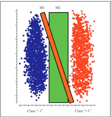
The concept of SVM is to classify each data sample into one of two categories: positive class denoted by “+1” and negative class denoted by “–1”. It boils down to find a de-cision boundary – a plane (a hyperplane forn>3), which divides data into two sets, one for each class. Next, all the measurements on one side of the determined boundary are
Class “–1”
Class “+1” Decision boundaries
Fig. 2. Binary classification.
classified as belonging to “+1” class and all those on the other side as belonging to “–1” class.
The problem is that many hyperplanes that divides the dataset can be determined (see Fig. 2). Hence, the best one has to be selected. In general, SVM tries to learn the decision boundary, which gives the best generaliza-tion. A good separation is achieved by the hyperplane that has the largest distance to the nearest data sample of any class – a wider margin implies the lower generalization error of the classifier [1], [23] (Fig. 3). To select the
max-M1 M2
Class “–1” Class “+1”
imum margin hyperplane the optimization problem is for-mulated and solved.
Let us focus on the SVM algorithm. Under the assump-tion that two classes +1 and –1 are considered the training setDofNpairs (xi,yi),i=1, . . . ,N, which is used during the training process can be defined as follows [24]:
D=n(xi,yi)|xi∈Rn,yi∈ {−1,+1}
oN
i=1, (4)
where xi denotes a training sample – fixed-length vector consisting of n values (measurements) and yi is a binary label associated to thei-th vector.
Given a training dataset, the SVM algorithm searches for a plane (a hyperplane for n>3) in the input space that separates the positive samples from the negative ones. Let us focus on the original SVM model developed by Vapnik [21] – linear classifier. Assume that all hyperplane inRnare parameterized by a vector w, and a constantb
wTx+b=0, (5)
wherew is the vector orthogonal to the hyperplane andb denotes the width of a margin.
For hyperplane(w,b)defined in Eq. (5) that separates the data the classification rule can be formulated:
hw(x) =sign(wTx+b). (6)
The functionhw should correctly classify the training data. Moreover, it should classify the other data that has not been known yet. The problem is that many such hyperplane can be found, i.e., all expressed by pairs(αw,αb)for each pos-itive constantα∈R+, and the optimal one should be se-lected. Therefore, as it has already been mentioned training a binary classification SVM means solving the optimiza-tion problem, which soluoptimiza-tion should be a maximum margin hyperplane (Fig. 3). For a given training setD defined in Eq. (4) the optimization problem is formulated [21]:
min w,b,ζ 1 2w Tw+C N
∑
i=1 ζi, (7)subject to the constraints:
yi(wTxi+b)≥1−ζi, ζi≥0, (8)
where ζi denotes the slack variable, which measures the degree of misclassification of the samplexi. C>0 is the constant value, which can be seen as a tunable parameter. The higher value ofCinvolves more importance on classi-fying all the training data correctly. The lower value ofC involves a more flexible hyperplane that tries to minimize the margin error. The quadratic programming can be used to calculate the optimal decision hyperplane [24], [25]. The next step is the prediction process. The goal is to classify each sample from the testing dataset on one side of the determined decision hyperplane as belonging to “–1” class and each that on the other side as belonging to “+1” class [26], [27]. Hence, the final goal of SVM is to produce
a model (based on the training data), which classifies the samples from a new dataset based only on the knowledge about their features and attributes.
In practical applications, it often happens that the datasets are not linearly separable in the data space. Due to the fact that the separation is easier in the higher space the solution of this problem is to map the original finite-dimensional space into a much higher-dimensional space (even infinite). Hence, the solution to create nonlinear classifiers by apply-ing kernel functions to maximum-margin hyperplanes was developed [28]–[30]. A kernel function K(xi,xj) defines the similarity between a given pair of objects. A large value of K(xi,xj) indicates that xi and xj are similar and a small value indicates that they are dissimilar.
Summarizing, the resulting nonlinear SVM algorithm is formally similar – every dot product in (8) is replaced by a nonlinear kernel function. Various kernel functions are employed. They are described in literature [31], [32]. The authors used the polynomial kernel function
K(xi,xj) = (γxTixj+r)d, γ>0 (9) to malware analysis. In Eq. (9) γ,r, andd denote kernel parameters. The other kernel functions widely used in the literature are as follows:
• radial basis function (RBF): K(xi,xj) =exp(γkxixjk2), γ>0,
• sigmoid:
K(xi,xj) =tanh(γxTixj+r), γ>0.
5. Case Study Results
5.1. Input DatasetThekNN, NB and SVM methods were used to classify
het-erogeneous data from the real malware database of the n6 platform. The n6 platform was developed in Research and Academic Computer Network (NASK) [33]. The purpose of the system is to monitor computer networks, collect, and analyze data about such events as threads, incidents, etc. [15].
Data in the n6 database are taken from a numerous sources and distributed channels. Events are detected by the de-vices located in many units and organizations (e.g. secu-rity organizations, software providers, independent experts, etc.) and monitoring systems serviced by CERT Poland (Computer Emergency Team Poland). Access to all col-lected datasets, i.e., URLs of malicious websites, addresses of infected machines, open DNS resolvers, etc., is pro-vided through a REST API. The API exposes an unified data model. Hence, the collected data is represented as a searchable collection of atomic events with a flexible set of properties (key-value pairs) with predefined seman-tics. The native output extension is JSON [RFC7159], al-though n6 supports other extensions, i.e., CSV [RFC4180] and IODEF [RFC5070]. A fine-grained permission model
and mandatory TLS [RFC2246] with client certificates for authentication and confidentiality are provided to control the access to the system (see Fig. 4).
Security data providers - URL-s - domains - IP adresses - malware - others H T T P S ISPs CSPs CERTs Banks
n6
ENGINEFig. 4. The n6 database.
Most of the data collected in the n6 database is updated daily. The n6 platform provides tools for sorting the in-cidents. Due to a sophisticated tagging system, incidents can be assigned to unique entities (e.g. based on IP address and AS numbers). Data are collected into special pack-age, which keeps an original source format (each source in separate file). Additionally it is possible to provide other information, e.g., about C & C servers that are not consisted in a client network, but can be utilized to detect infected computers. Information about malicious sources is trans-ferred by the platform as URL’s, domain, IP addresses or names of malware.
5.2. Training Dataset Analysis and Visualization
The preliminary analysis of the training dataset was per-formed. Four attributes are assigned to each sample col-lected in the n6 database: time, format, domain, and ad-dress. The recordtime consists of two components: date
and time of inserting an event into the n6 database. To simplify the analysis two attributes were transformed to the
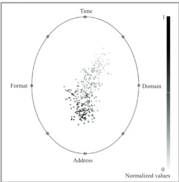
Time Format Domain Address Normalized values 0 1
Fig. 5. n6 dataset visualization (radius visualization).
more suitable forms. Eachdomain attribute was clustered,
and converted to the numerical. Each IP address was
de-scribed in decimal according to the formula: W.X.Y.Z=
2563W+2562X+256Y+Z, where W,X,Y,Z correspond with values in IP address.
Then, the data samples from the training dataset were ana-lyzed. The visualization of all attributes, i.e., format, time, domain, and address are displayed in Figs. 5 and 6. Prior to visualization, values of attributes are scaled to the val-ues between 0 and 1. The widely used non-linear multi-dimensional visualization technique Radviz [34] was used to present the data in the four-dimensional space defined by these attributes. In this approach, all attributes are pre-sented as anchor points equally spaced around the perime-ter of a unit circle (Fig. 5). Data samples are shown as points inside the circle. Their positions are determined by a metaphor from physics: each point is held in place with springs that are attached at the other end to the attribute anchors. The stiffness of each spring is proportional to the value of the corresponding attribute and the point ends up at the position where the spring forces are in equilibrium. Data samples that are close to a given anchor have higher values of this attribute. We can determine some groups of samples with similar values of all attributes.
address domain format
Fig. 6. n6 dataset visualization (self-organizing map).
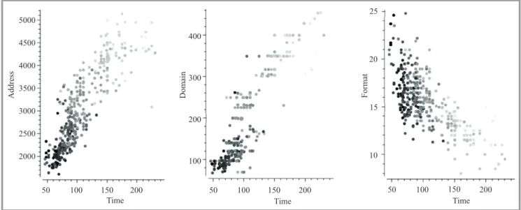
Next, the self-organizing map (SOM) – another technique for displaying multidimensional data – was applied to in-vestigate the general structure of the training dataset. The map depicted in Fig. 6 shows the distribution of samples in the dataset mapped into the space of all attributes. Figure 7 presents the correlations between time attribute
and three other, i.e., format, domain and address. It can
be observed that all attributes are commonly correlated, and the correlation coefficient for each pair of attributes is different. Correlations between format and domain versus
50 100 150 200 Time 25 20 15 10 Format 50 100 150 200 Time 400 300 200 100 Domain 50 100 150 200 Time 5000 4500 4000 3500 3000 2500 2000 Address
Fig. 7. Correlations between time and other attributes.
time are positive (rising), and for address versus time is negative (falling).
5.3. Validation of Classification Systems and Comparative Study
The goal of the experiments was to validate thekNN, NB
and SVM classification systems on datasets taken from the n6 platform. Three series of experiments were performed for the same input dataset consisting of 398 samples. The goal of all tests was to classify each data sample from the input dataset into one of two categories: positive class de-noted by “+1” (normal data) and negative class dede-noted
Table 1
Confusion matrix forkNN classification
Class CV [%] LOO [%] RS [%]
+1 –1 +1 –1 +1 –1
+1 94.4 7.6 94.3 8.3 96.0 13.7
–1 5.6 92.4 5.7 91.7 4.0 86.3
Table 2
Confusion matrix for NB classification
Class CV [%] LOO [%] RS [%]
+1 –1 +1 –1 +1 –1
+1 96.6 6.6 96.9 7.2 96.2 8.7
–1 3.4 93.4 3.1 92.8 3.8 91.3
Table 3
Confusion matrix for SVM classification
Class CV [%] LOO [%] RS [%]
+1 1 +1 –1 +1 –1
+1 98.1 13.9 95.4 7.3 99.2 11.8
–1 1.9 86.1 4.6 92.7 0.8 88.2
by “–1” (malicious data). The accuracy of the classifica-tion was evaluated and efficiency of kNN, NB and SVM
techniques was compared (Tables 1–3). Parameters of the techniques equals respectively: number of neighbors were k=3 in Euclidean metrics for kNN, Laplace probability estimation and size of LOESS window equals 0.5 for NB and for SVM the polynomial kernel function was used with parametersγ=0.5,r=1andd=3.
Three commonly used cross-validation methods were used for assessing how the results of the classification will gen-eralize to an independent data sets [4], [23]: CV – Cross Validation, LOO – Leave-One-Out and RS – Random Sam-pling. Multiple tests for various parameters of these meth-ods were performed. In this paper the results obtained for 5-folds cross validation and random sampling with 5 repe-titions of training process and 50% of the relating training set size is presented. For these values of parameters, the au-thors got the best compromise between accuracy and speed of calculations.
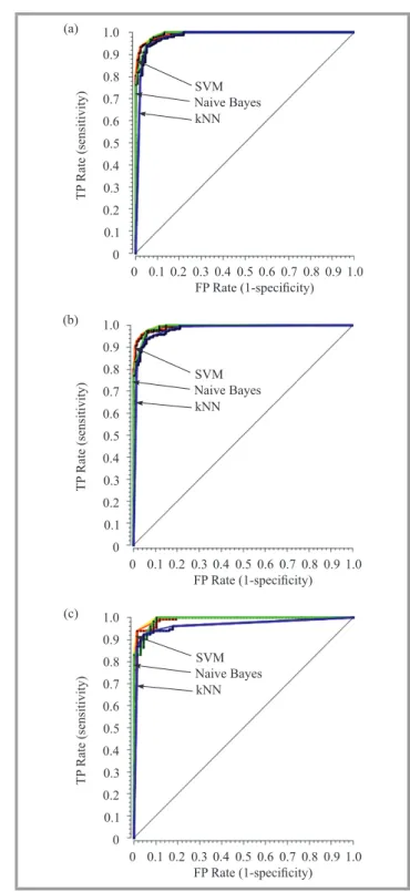
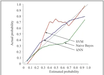
The achieved efficiency of fitting of the testing data was from 86 to 99% respective to the given method and class (+1 or –1). The SVM method gave the best accuracy of selecting to the class “+1” (99.2% for RS technique). Figure 8 shows the calibration plots that illustrate the qual-ity of thekNN, NB and SVM based classification systems
the classification systems. Figure 9 displays the receiver operating characteristic curves (ROC) for these systems. Then, the quality of the classification systems was as-sessed. Five commonly used criteria were taken into con-sideration:
– CA – classification accuracy, – Sens – sensitivity,
– Spec – specificity,
– AUC – area under ROC curve, – F1 – F-measure.
1.0 0.9 0.8 0.7 0.6 0.5 0.4 0.3 0.2 0.1 0 0 0.1 0.2 0.3 0.4 0.5 0.6 0.7 0.8 0.9 1.0 (a) Actual probability kNN SVM Naive Bayes Estimated probability 1.0 0.9 0.8 0.7 0.6 0.5 0.4 0.3 0.2 0.1 0 0 0.1 0.2 0.3 0.4 0.5 0.6 0.7 0.8 0.9 1.0 (b) Actual probability Estimated probability kNN SVM Naive Bayes 1.0 0.9 0.8 0.7 0.6 0.5 0.4 0.3 0.2 0.1 0 0 0.1 0.2 0.3 0.4 0.5 0.6 0.7 0.8 0.9 1.0 (c) Actual probability Estimated probability kNN SVM Naive Bayes
Fig. 8. Calibration plots forkNN, NB and SVM based systems:
(a) CV, (b) LOO, (c) RS.
The sensitivity of learning machine (Sens) is defined as follows:
Sens= T P
T P+FP, (10)
whereT P denotes the number of true positive predictions andFPthe number of false positive predictions.
The specificity of learning machine (Spec) is defined as follows: S pec= T N T N+FN, (11) TP Rate (sensitivity) TP Rate (sensitivity) TP Rate (sensitivity) 1.0 0.9 0.8 0.7 0.6 0.5 0.4 0.3 0.2 0.1 0 0 0.1 0.2 0.3 0.4 0.5 0.6 0.7 0.8 0.9 1.0 kNN SVM Naive Bayes
FP Rate (1-specificity) 1.0 0.9 0.8 0.7 0.6 0.5 0.4 0.3 0.2 0.1 0 0 0.1 0.2 0.3 0.4 0.5 0.6 0.7 0.8 0.9 1.0 FP Rate (1-specificity) 1.0 0.9 0.8 0.7 0.6 0.5 0.4 0.3 0.2 0.1 0 0 0.1 0.2 0.3 0.4 0.5 0.6 0.7 0.8 0.9 1.0 FP Rate (1-specificity) (a) (b) (c) kNN kNN SVM SVM Naive Bayes Naive Bayes
Fig. 9. Receiver operating characteristic curves forkNN, NB and
SVM based systems: (a) CV, (b) LOO, (c) RS.
whereT Ndenotes the number of true negative predictions andFN the number of false negative predictions.
The classification accuracy (CA) is defined by the ratio of number of correctly identified samples into the size of the dataset.
CA= T P+T N
T N+FN+T P+FP. (12)
The accuracy of a test (AUC) depends on how well the test separates the data samples being tested. The accuracy is
measured by the area under the ROC (Receiver Operating Characteristic) curve plotted in the coordinate system with x-axis corresponding to the probability of false positive se-lection andy-axis corresponding to the probability of true positive selection. In this research, x-axis corresponds to the false alarm andy-axis to the true malware detection. In general, an area of 1 represents a perfect test; an area of 0.5 represents a worthless test. F-measure is a measure of a test’s accuracy. It considers both the precision p (ratio of the number of correct results to the number of returned results) and the recall r (ratio of the number of correct results to the number of results that should have been re-turned) of the test to compute the score. The F-measure can be interpreted as a weighted average of the precision and recall, where the F-measure reaches its best value at 1 and worst score at 0.
The values of CA, Sens, Spec, AUC and F1 criteria calculated forkNN, NB and SVM based classification
sys-tems are collected in Table 4. Table 4
Evaluation ofkNN, NB, and SVM classification
Method CV LOO RS kNN CA 0.9371 0.9347 0.9246 Sens 0.9617 0.9579 0.9237 Spec 0.8905 0.8905 0.9265 AUC 0.9776 0.9788 0.9631 F1 0.9526 0.9506 0.9416 NB CA 0.9548 0.9548 0.9447 Sens 0.9655 0.9617 09542 Spec 0.9343 0.9416 0.9265 AUC 0.9910 0.9912 0.9898 F1 0.9655 0.9654 0.9579 SVM CA 0.9398 0.9422 0.9497 Sens 0.9808 0.9732 09774 Spec 0.8613 0.8832 0.8971 AUC 0.9937 0.9927 0.9907 F1 0.9552 0.9567 0.9623
The results for all validation experiments confirm a good quality of our classification systems. The obtained classifi-cation accuracy was from about 92 to 95%, sensitivity from 92 to 98%, and specificity from 86 to 94%. All validation experiments gave the similar results. However, the slight better specificity was obtained for NB, while sensitivity was the best for SVM.
5.4. Application of Classification Systems to Malware Detection
Finally, thekNN, NB and SVM based classification systems
were used to malware detection. The systems trained on the training dataset consisting of 398 samples (the same that
used in the experiments described in the previous section) were used to classify dataset consisting of 10747 samples. Hence, in contrary to the validation tests the training dataset was about five times smaller than the testing one. More-over, both training and testing datasets contained different measurements.
The results of data classification are presented in Table 5. The quality of the classification systems is presented in Figs. 10 and 11 and Table 6. Figure 10 displays the ob-tained receiver operating characteristic curves (ROC) for all systems. Figure 11 shows the calibration plots.
Table 5
Confusion matrices (three classification systems)
Class kNN [%] NB [%] SVM [%] +1 –1 +1 –1 +1 –1 +1 58.4 8.2 73.8 15.2 76.1 15.3 –1 41.6 91.8 26.2 84.8 23.9 84.7 TP Rate (sensitivity) 1.0 0.9 0.8 0.7 0.6 0.5 0.4 0.3 0.2 0.1 0 0 0.1 0.2 0.3 0.4 0.5 0.6 0.7 0.8 0.9 1.0 kNN SVM Naive Bayes FP Rate (1-specificity)
Fig. 10. Receiver operating characteristic curves forkNN, NB
and SVM based systems.
Actual probability Estimated probability 1.0 0.9 0.8 0.7 0.6 0.5 0.4 0.3 0.2 0.1 0 0 0.1 0.2 0.3 0.4 0.5 0.6 0.7 0.8 0.9 1.0 kNN SVM Naive Bayes
Fig. 11. Calibration plots forkNN, NB and SVM based systems. The values of CA, Sens, Spec, AUC and F1 criteria calcu-lated for thekNN, NB and SVM based systems are collected
Table 6
Evaluation of classification systems
Validation criterion kNN NB SVM CA 0.8117 0.8311 0.8342 Sens 0.4661 0.7669 0.4576 Spec 0.8259 0.9474 0.9641 AUC 0.8736 0.8991 0.8637 F1 0.5714 0.6630 0.5714
Next, the performance of the NB,kNN and SVN based
clas-sification systems was compared. Table 7 collects the train-ing and classification times for all methods. The efficien-cies ofkNN and SVM are similar (training: 0.31–0.33 s,
classification: 1.71–2.11 s). Both methods provide satisfac-tory results. It is obvious that the complexity of these meth-ods depends on the assumed number of neighbors (kNN)
and employed kernel core function (SVM). NB based clas-sification system is much slower, and its execution time strongly depends on the size of a dataset.
Table 7
Training and classification times
Techniques kNN NB SVM
ttraining [s] 17.21 5.91 5.03
tclassi f ication [s] 30.00 5.33 10.05
In general, the results presented in the tables and figures show that the classification systems employingkNN, NB
and SVM methods provide a good accuracy classification (CA more than 80%). However, the results are of course much worse than in case of cross-validation experiments. The largest differences are observed for the specificity cri-terion.
6. Summary and Conclusion
In this paper the authors consider the application of three types of supervised learning methods: k-Nearest
Neigh-bours, Naive Bayes, and Support Vector Machine to mal-ware detection systems. These methods were used to the classification of data on the Web into malware and clean class. The performance of the methods was validated. The commonly used validation techniques, i.e., k-folds
Cross-Validation, Leave One Out, and Random Sampling were applied.
Moreover, the systems were used to malware detection in real network. In general, the results of all experiments confirm that the examined classification methods achieve the relatively high level of accuracy, sensitivity, and speci-ficity. Therefore, it can be expected that these methods could be successfully implemented in intrusion detection systems. However, the size of training dataset, selection of methods and their parameters strongly influences the results of classification. Dealing with unstructured data
is the main strength of investigated methods especially in the case of computer network datasets that are frequently heterogeneous, unstructured and often incomplete. In au-thors opinion future work can be focused on optimization of calibration parameters in order to achieve better values of criteria.
Nevertheless, the computation of strong heterogeneous data, and pre-processing of this data is still heavy. There-fore, the classification of large dataset on the Web is still a challenging task. The further improvements of investi-gated methods are necessary to achieve efficient techniques for network security.
Acknowledgment
This research was partially supported by the “Nippon-European Cyberdefense – Oriented Multilayer threat Anal-ysis (NECOMA)” FP7 grant agreement number 608533 and research fellowship within Project “Information tech-nologies: Research and their interdisciplinary applications”, agreement number UDA POKL.04.01.01-00-051/10-00.
References
[1] T. Hastie, R. Tibshirani, and J. Friedman,The Elements of Statistical Learning, 2nd ed. Series in Statistics, Springer, 2009.
[2] W. S. Noble, “Support vector machine applications in
compu-tational biology”, in Kernel Methods in Computational Biology,
B. Schölkopf, K. Tsuda, and J.-P. Vert, Eds. Cambridge, USA: MIT Press, 2004, pp. 71–92.
[3] C. Wagner, G. Wagener, R. State, and T. Engel, “Malware analysis with graph kernels and support vector machines”, inProc. 4th Int. Conf. Malicious and Unwanted Software MALWARE 2009, Montreal, Canada, 2009, pp. 63–68.
[4] M. Krzyśko, W. Wołyński, T. Górecki, and M. Skorzybut, Systemy
uczące się(Learning systems). Warszawa: Wydawnictwo Naukowo Techniczne, 2009, pp. 107–187 (in Polish).
[5] K. Rieck, T. Holz, C. Willems, P. Dussel, and P. Laskov, “Learn-ing and classification of malware behavior”, inProc. 5th In. Conf. DIMVA 2008, Paris, France, 2008, vol. 5137, pp. 108–125. [6] M. Amanowicz and P. Gajewski, “Military communications and
in-formation systems interoperability”, inProc. Milit. Commun. Conf. MILCOM 96, McLean, VA, USA, 1996, vol. 1–3, pp. 280–283. [7] R. Kasprzyk and Z. Tarapata, “Graph-based optimization method
for information diffusion and attack durability in networks”, in Rough Sets and Current Trends in Computing, LNCS, vol. 6086, pp. 698–709, Springer, 2010.
[8] M. Mincer and E. Niewiadomska-Szynkiewicz, “Application of so-cial network analysis to the investigation of interpersonal connec-tions”,J. Telecommun. Inform. Technol., no. 2, pp. 81–89, 2012. [9] M. Shankarapani, K. Kancherla, S. Ramammoorthy, R. Movva, and
S. Mukkamala, “Kernel machines for malware classification and sim-ilarity analysis”, inProc. Int. Joint Conf. Neural Netw. IJCNN 2010, Barcelona, Spain, 2010, pp. 1–6.
[10] S. Forrest et al., “Self-nonself discrimination in a computer”, in Proc. Comp. Soc. Symp. Res. Secur. and Priv., Oakland, CA, USA, 1994, vol. 10, pp. 311–324.
[11] I. Liane de Oliveira, A. Ricardo, A. Gregio, and A. M. Cansian, “A malware detection system inspired on the human immune sys-tem”, inComputational Science and its Applications – ICCSA 2012, LNCS, vol. 7336, pp. 286–301, Springer, 2012.
[12] E. Stalmans and B. Irwin, “A framework for DNS based detection and mitigation of malware infections on a network”, in Proc.10th Ann. Inform. Secur. South Africa Conf. ISSA 2011, Johannesburg, South Africa, 2011.
[13] M. Zubair Shafiq, S. Ali Khayam, and M. Farooq, “Embedded
mal-ware detection using markov n-grams”, inDetection of Intrusions
and Malware, and Vulnerability Assessment, T. Holz and H. Bos, Eds.,LNCS, vol. 6739, pp. 88–107. Springer, 2008.
[14] M. Franklin, A. Halevy, and D. Maier. “From databases to
datas-paces: A new abstraction for information management”, Sigmod
Record, vol. 34, no. 4, pp. 27–33, 2005.
[15] K. Lasota and A. Kozakiewicz, “Analysis of the Similarities in
Ma-licious DNS Domain Names”, inSecure and Trust Computing, Data
Management and Applications, C. Lee, J.-M. Seigneur, J. J. Park,
and R.R. Wagner, Eds.Communications in Computer and
Informa-tion Science, vol. 187, pp. 1–6. Springer, 2011.
[16] Y. Yanfang, D. Wang, T. Li, and D. Ye, “IMDS: Intelligent
mal-ware detection system”, in Proc. 13th ACM SIGKDD Int. Conf.
Knowl. Discov. Data Mining KDD’07, San Jose, CA, USA, 2007, pp. 1043–1047.
[17] M. R. Faghani and H. Saidi, “Malware propagation in online social
networks”, inProc. Int. Conf. Malicious and Unwanted Software
MALWARE 2009, Montreal, Canada, 2009, pp. 8–14.
[18] P. Cunningham and S. J. Delany, “k-Nearest Neighbour Classifiers”, Tech. Rep. UCD-CSI-2007-4, UCD School of Computer Science and Informatics, Dublin, 2007, pp. 1–17.
[19] J. M. Keller, “A fuzzyk-Nearest Neighbor algorithm”,IEEE Trans. Syst., Man, and Cybernet., vol. 15, no. 4, pp. 580–585, 1985. [20] L. Jiang, H. Zhang and Z. Cai “A Novel Bayes Model: Hidden
Naive Bayes”, IEEE Trans. Knowl. Data Engin., vol. 21, no. 10,
pp. 1361–1371, 2009.
[21] V. N. Vapnik,The Nature of Statistical Learning Theory. New York: Springer, 1995.
[22] A. Borders and L. Bottou, “The Huller: a simple and efficient
on-line SVM”, in Machine Learning: ECML-2005, J. Gama, R.
Ca-macho, P. Brazdil, A. Jorge, and L. Torgo, Eds.,LNCS, vol. 3720, pp. 505–512. Springer, 2005.
[23] J. Koronacki and J. Ćwik,Statystyczne systemy uczące się(Statistical learning systems). Warsaw: Exit, 2008 (in Polish).
[24] T. Joachims, “Support Vector and Kernel Methods”, SIGIR-Tutorial, Cornell University Computer Science Department, 2003.
[25] N. Cristianini and J. Shawe-Taylor,An Introduction to Support Vector Machines, 1st ed. Cambridge University Press, 2000, pp. 25–29. [26] E. Ikonomowska, D. Gorgevik, and S. Loskovska, “A survey of
stream data mining”, in Proc. 8th Nat. Conf. Int. Particip. ETAI
2007, Ohrid, Republic of Macedonia, 2007, pp. 16–20.
[27] T. Joachims, “Training linear SVMs in linear time”, inProc. 12th ACM SIGKDD Int. Conf. Knowl. Discov. Data Mining KDD 2006, Philadelphia, PA, USA, 2006 pp. 217–226.
[28] Kernel Machines homepage [Online]. Available: http://www.kernel-machines.org/
[29] C. Burges, “A Tutorial on Support Vector Machines for
Pat-tern Recognition”, Knowledge Discovery and Data Mining, vol. 2,
no. 2, pp. 121–167, 1998.
[30] T. Jebara, “Multi-task feature and kernel selection for SVMs”, in Proc. Int. Conf. on Machine Learning, Banff, Canada, 2004, pp. 55–63.
[31] F. R. Bach, G. Lanckriet, and M. Jordan “Multiple kernel learn-ing, conic duality and the smo algorithm”, inProc. 21st Int. Conf. Machine Learning ICML’04, Banff, Canada, 2004, pp. 6–13. [32] F. R. Bach, R. Thibaux, and M. I. Jordan, “Computing regularization
paths for learning multiple kernels” inAdvances in Neural Informa-tion Processing Systems, L. K. Saul, Y. Weiss, and L. Bottou, Eds. MIT Press, 2005, pp. 73–80.
[33] N6 Platform homepage [Online]. Available: http://www.cert.pl/news/tag/n6
[34] G. M. Draper, “Interactive radial vizualizations for information re-trieval and management”, Ph.D. Thesis, Univertity of Utah, 2009, Chapter 3.
Michał Kruczkowski received his M.Sc. in Electronics and Telecommunications from the Gdańsk University of Technol-ogy in 2011. Currently he is a Ph.D. student at the Insti-tute of Computer Science, Pol-ish Academy of Sciences. Since 2013 he works at the Research and Academic Computer Net-work (NASK). His research in-terests focus on artificial intelligence, analysis of strongly heterogeneous datasets, advanced statistical models, ma-chine learning.
E-mail: [email protected]
Research and Academic Computer Network (NASK) Wąwozowa st 18
02-796 Warsaw, Poland
E-mail: [email protected] Institute of Computer Science
Polish Academy of Sciences Jana Kazimierza st 5 01-248 Warsaw, Poland
Ewa Niewiadomska-Szynkie-wicz D.Sc. (2005), Ph.D. (1995), professor of control and computer engineering at the Warsaw University of Tech-nology, head of the Complex Systems Group. She is also the Director for Research of Re-search and Academic Computer Network (NASK). The author and co-author of three books and over 140 journal and conference papers. Her research interests focus on complex systems modeling, optimization and control, computer simulation, parallel computation, computer networks and ad hoc networks. She was involved in a number of research projects including EU projects, coordinated the Groups activities, managed organization of a number of national-level and international conferences. E-mail: [email protected]
Institute of Control and Computation Engineering Warsaw University of Technology
Nowowiejska st 15/19 00-665 Warsaw, Poland E-mail: [email protected]
Research and Academic Computer Network (NASK) Wąwozowa st 18