Forecasting with many predictors using message passing algorithms

(1)

Essex Finance Centre

Working Paper Series

Working Paper No18: 04-2017

“Forecasting with many predictors using message passing

algorithms”

“Dimitris Korobilis”

Essex Business School, University of Essex, Wivenhoe Park, Colchester, CO4 3SQ Web site: http://www.essex.ac.uk/ebs/

(2)

Forecasting with many predictors using message passing

algorithms

Dimitris Korobilis University of Essex April 27, 2017 Abstract

Machine learning methods are becoming increasingly popular in economics, due to the increased availability of large datasets. In this paper I evaluate a recently proposed algorithm calledGeneralized Approximate Message Passing (GAMP), which has been very popular in signal processing and compressive sensing. I show how this algorithm can be combined with Bayesian hierarchical shrinkage priors typically used in economic forecasting, resulting in computationally efficient schemes for estimating high-dimensional regression models. Using Monte Carlo simulations I establish that in certain scenarios GAMP can achieve estimation accuracy comparable to traditional Markov chain Monte Carlo methods, at a tiny fraction of the computing time. In a forecasting exercise involving a large set of orthogonal macroeconomic predictors, I show that Bayesian shrinkage estimators based on GAMP perform very well compared to a large set of alternatives.

Keywords: high-dimensional inference; compressive sensing; belief propagation; Bayesian shrinkage; dynamic factor models

(3)

1 Introduction

Increased availability of large datasets is both a blessing and a curse for macroeocnomists and financial analysts. It is a blessing because we currently have so many advanced statistical methods and computational tools that allow us to uncover new stylized facts from disaggregated and other high-dimensional datasets, that economists of the past didn’t have the chance to consider. It is a curse because policy-makers and analysts cannot any more make decisions based on a handful of preferred indicators, rather, they have to monitor hundreds or thousands of variables, which can be costly to maintain and hard to interpret. As a consequence, given that data availability increases at a polynomial rate, a major challenge for modern economists and econometricians is to design estimation algorithms that i) are able to separate the “signal” from the “noise” in a high-dimensional dataset, and ii) are computationally efficient in order to support real-time decision making by policy-makers and analysts. The purpose of this paper is to introduce to the economics literature a machine learning algorithm that can be used to perform dynamic programming, maximum likelihood estimation, and Bayesian inference using shrinkage priors. The so-called Generalized Approximate Message Passing (GAMP) has been proposed by Rangan (2011), and is an algorithm that extends the Approximate Message Passing (AMP) algorithm of Donoho, Maleki and Montanari (2009). In turn these are fast, approximate versions of general message passing algorithms used in machine learning; see Barber (2012) for an insightful introduction to this literature.

There is more than one way to motivate message passing methods. For example, Donoho, Maleki and Montanari (2011) motivate AMP as an iterative thresholding algorithm that is a fast alternative to convex optimization and linear programming methods; see also Bayati and Montanari (2011). In fact, all variants of message passing algorithms are dynamic programming methods designed for efficiently performing large computations by distributing calculations among a number of simpler processors. Here, I build on Rangan (2011) and present an intuitive derivation of generalized approximate message passing based on graphical methods. My starting point is a Bayesian factor graph (Kschischang, Frey and Loeliger, 2001), that is, a

(4)

graphical representation of the posterior probability function of the regression coefficients using nodes and edges. Such graphical representation of a probabilistic model allows factorizations (decompositions) of the parameter posterior distribution into simpler probability functions. These factorizations are basically probability rules that define how a “message is passed” from one node of the graph to the next. The basic idea behind such decompositions in factor graphs is that of the distributive law:

a·b+a·c=a(b+c). (1)

In terms of the variables a, b, c, the axiom above implies one less operation on the right hand side. In terms of probability distributions we can derive similar factorizations that could result - in high-dimensional spaces - in huge savings in computing power.

It becomes, therefore, apparent that GAMP can be thought of as an algorithm that breaks down the problem of estimating a high-dimensional parameter vector into smaller, more accessible problems. This is achieved by factorizing the high-dimensional Bayesian parameter posterior into approximate, analytical expressions for the marginal parameter posteriors. Put differently, if one is faced with the problem of estimating a p-dimensional vector of parameters β, GAMP allows to obtain approximate expressions for the posteriors of each element βi for i= 1, ..., p1. While the next section outlines the exact mechanics behind such approximations, three questions immediately arise: i) how accurate these approximations are, ii) how adaptable and versatile the algorithm is in various modelling scenarios, and iii) what are the computational gains compared to existing algorithms? This paper aims to give detailed answers to all these questions.

First I show that GAMP can be combined with, among others, Normal-Gamma shrinkage priors (Griffin and Brown, 2010) as well as variable selection priors (George and McCulloch, 1993). While GAMP only provides the solution to sparse regression coefficients, any additional parameters involved in an econometric model, such as a regression variance, can be updated using the EM algorithm. Next, I perform a Monte Carlo experiment where I generate data

1

The exact marginal posterior ofβiinvolves calculating ap−1 multidimensional integral, since this posterior

is obtained after “marginalizing” the impact of the remainingp−1 elements ofβ. Whenpis large, computing such integrals is impossible, even for simple regression models.

(5)

from sparse regression models in order to evaluate the numerical stability and computational efficiency of GAMP. GAMP-based algorithms perform at least as well, or better in several cases, than MCMC-based shrinkage algorithms2 in recovering the true regression coefficients, at a fraction of the computing time. Finally, the precision and usefulness of GAMP is evaluated in an extensive forecasting exercise following closely Stock and Watson (2012). This exercise involves estimating univariate regression models for forecasting 222 quarterly US macroeconomic series using a large set of orthogonal predictors, typically in the form of factors (principal components). Under a wide-range of alternative shrinkage algorithms (Bayesian MCMC-based algorithms, bootstrap aggregation, and naive approaches) the proposed GAMP-based algorithms perform extremely well. The results are robust both when looking at all 222 series as well as a selection of 14 important series (such as GDP, employment, IP, CPI inflation, Federal funds rate, SP500 returns etc), and under both recursive and rolling forecasting schemes. Therefore, this paper makes a strong case in establishing GAMP-based algorithms as a significant and “low-cost” (in terms of requirements in tuning, computational resources, and maintenance/updating) tool for macroeconomic forecasting using many predictors, and for general monitoring of large datasets.

In the next section I outline this new methdology using Bayesian arguments, and I explain the intuition behind the approximations to marginal posterior distributions achieved using GAMP. I also discuss convergence issues and demonstrate the kind of shrinkage and variable selection priors one can combine with GAMP. Next, in section 3 I provide results of the Monte Carlo study, and in section 4 I implement the large-scale forecasting exercise. Section 5 concludes the paper with an evaluation of GAMP and with thoughts for future incorporation of GAMP in other models and settings that economists are interested in (such as vector autoregressions).

2_{In particular, I contrast to the Bayesian lasso (Park and Casella, 2008) and stochastic search variable} selection (SSVS; George and McCulloch, 1993).

(6)

2 Methodology

The starting point is the following regression model in vector/matrix form

y=xβ+ε (2)

where y is a T ×1 vector of the variable of interest, x is a T ×p matrix of predictors (possibly including lags of y), β is a p×1 vector of coefficients, and ε ∼ N 0, σ2IT

. A motivating assumption for considering estimation algorithms that perform shrinkage and are computationally efficient is thatpT, that is, the specification in equation (2) can be thought of as a regression with more predictors than observations. However, I will subsequently show that GAMP performs very well in any “large p” regression case, even if p < T. Note that when estimating a regression interest also lies in the estimation ofσ2, but I first consider this parameter to be known and I subsequently discuss joint estimation ofβ, σ2later in this section. Let us consider first an independent (but not necessarily i.i.d) prior for β, denoted p(β) =

Qp

i=1p(βi), and the resulting posterior from Bayes Theorem

p(β|y) ∝ p(y|β)p(β) (3) = T Y t=1 p(yt|β) p Y i=1 p(βi). (4)

The exact marginal posterior for βi,i= 1, ..., p is of the form

p(βi|y) = Z p(β|y)dβj6=i, (5) ∝ Z p(y|β)p(β)dβj6=i, (6) = p(βi) Z p(y|β) p Y j=1,j6=i p(βj)dβj6=i, (7)

wheredβj6=i denotes integration over the whole set ofp−1 parameters βj forj6=i. Therefore, the formula above requires integration over a (p−1)-dimensional integral, a numerical problem

(7)

that can become computationally infeasible for high-dimensional vectorsβ.

2.1 Generalized Approximate Message Passing

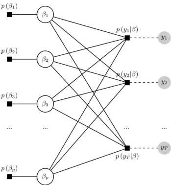
The computationally efficient GAMP algorithm approximations can be motivated using factor graphs, that is, graphical models that allow to factorize random variables into lower-dimensional quantities. In our case, the random variable we want to factorize is the high-dimensional parameter posterior β. Based on Bayes Theorem above, the resulting factor graph is depicted in Figure 1. This graph consists of variable vertices β = (β1, ..., βp) which are denoted with a white circle, and function vertices f = [p(β), p(y|β)] = [p(β1), ..., p(βp), p(y1|β), ..., p(yT|β)] which are represented using filled boxes. I denote by µ_p₍•)→a the message passed from probability function p(•) to random variable a, and vice-versa for the message µa→p(•). We are now able to redefine the marginal posterior of βi, presented in equation (7), as the product of incoming messages at nodeβi in the graph

p(βi|y) =µp(βi)→βi T Y

t=1

µ_p₍_y_t|β)→βi. (8)

The message µp(βi)→βi is simply the prior distribution p(βi). According to the sum-product

message rule, the term inside the product can be decomposed as

µ_p₍_y_t|β)→βi = Z p(yt|β) p Y j=1,j6=i µ_β_j→p(yt|β)dβj6=i. (9)

In the decomposition above, the message from node βj to function p(yt|β) is the product of all incoming messages to node βi, excluding the message coming fromp(yt|β) itself

µβj→p(yt|β)=p(βj) T Y

s=1,s6=t

µp(ys|β)→βj. (10)

We can see in equations (9)-(10) that in order to obtain the message µ_p₍_y_t|β)→βi we need µ_β_j→p(yt|β) and vice-versa. Therefore, one can simply update both equations iteratively, using a scheme that is called Belief Propagation (BP; see Pearl, 1982) and consists of the following

(8)

p(β1) β1 p(y1|β) y1 p(β2) β2 p(y2|β) y2 p(β3) β3 ... ... ... ... p(yT|β) yT p(βp) βp

Figure 1: Factor graph for the posterior distribution ofβ

where superscript (r) denotes the rth iteration of the algorithm. In graphs with a tree structure, one iteration of the algorithm above can recover the exact marginal posteriors for the parameters βi. In a factor graph with loops, that is, when a message can start from a given node and return to the same node using various alternative paths, the BP algorithm can sometimes achieve a good approximation. This algorithmic issue is discussed in the following subsection.

From that point onward the GAMP algorithm can be derived by introducing two further approximations to the BP iterations. First, when p → ∞ a central limit theorem

(9)

(CLT) postulates that the messages Qp

j=1,j6=iµβj→p(yt|β) can be approximated by a Gaussian distribution with respect to the uniform norm 3. This result means that both messages in (9)-(10) can be represented as products of Gaussian distributions. A second approximation involves taking the Taylor-series expansion of terms in the messages, so that the mean and variance of p(βi|y) can be obtained analytically up to the omission of O(1/p) terms. Exact derivation of these steps involve many tedious steps, and the reader is referred to the Technical Appendix of Rangan (2011) for more details. What is important to stress at this point is that both the CLT and Taylor-series approximations vanish as p → ∞ with p/T → δ for some constant δ; see Rangan (2011) for more details. This is an example of the “blessing of Big Data”, and the GAMP algorithm fully facilitates the largep asymptotics.

The final product of all the approximations to the two Belief Propagation update rules of equations (11) - (12), is a simple iterative algorithm that provides marginal parameter posteriors of βi and zt, where define zt = Xtβ and assume, without loss of generality4, that Xt∼N 0, T−1I

. In particular, GAMP approximatesp(βi|y) with

p(βi|y, qi, τq,i) =

p(βi)N(βi|qi, τq,i) R

βp(βi)N(βi|qi, τq,i)

, (13)

where ct, τc,t are also computed iteratively and more details can be found in the Techincal Appendix.

3

This is a result of the Berry-Esseen central limit theorem which states that a sum of random variables converge to a Gaussian density; see a proof of that theorem in Donoho, Maleki and Montanari (2010). Given that the Belief Propagation equations involve products of random variables, rather than sums, derivations of GAMP based on this central limit theorem typically proceed by taking logarithms of equations (8)-(10). The marginal posteriorp(βi|y) is then recovered by performing an exponential transformation of the log messages,

and by normalizing so that the posterior integrates to one.

4_{As Donoho, Maleki and Montanari (2010) show, one can relax this assumption and consider other} distributions; see also Bayati and Montanari (2011).

(10)

2.2 Stability of GAMP

The GAMP algorithm, whose steps are provided in detail in the Technical Appendix, iterates through simple scalar multiplications and additions that result in a total of O(T p) algorithmic operations. That is, estimation of the marginal parameter posterior distribution does not involve any matrix inversion that is typically met in many forms of parametric estimation algorithms. Convergence is achieved when the difference between estimates of the posterior mean ofβbetween two consecutive iterations is below a pre-specified tolerance level. Therefore, an important question is whether there are theoretical guarantees that the algorithm will converge. The answer is partly yes. In graphs with loops, such as the one specified in the previous section, the Belief Propagation algorithm will approximate the marginal posterior distribution forβiby only considering its dependence on its direct neighbours. What this means in practical terms is that all the factorizations of distributions resulting from BP implicitly assume that there is a low correlation between thep elements β and, as a consequence, thep columns ofX. In general, many MCMC-based variable selection and shrinkage algorithms also suffer from the presence of highly correlated predictors. However, GAMP, due to its underlying approximate factorizations, has even lower threshold for handling correlated data. In the next section I show using Monte Carlo experiments that GAMP in the case of regressions with mildly correlated predictors can achieve estimation accuracy comparable to MCMC, at a fraction of the computing time5. Additionally, the empirical exercise involves regressions with orthogonal predictors such as principal components, or predictors that have been orthogonalized (that is, rotated and rescaled such thatx∼iid(0, Ip)) prior to estimation.

2.3 Joint Parameter Estimation

A salient feature of the derivations above is that they are also valid when the prior on β is conditional on some hyperparameters θ, that is when the prior is of the general hierarchical

5_{Additionally, there is a large literature in engineering documenting that loopy BP works very well in various} applications including turbo decoding (McEliece et al., 1998), computer vision (Freeman et al., 2000), and compressed sensing (Baron et al., 2010).

(11)

form

p(β, θ) =p(β|θ)p(θ). (15)

In this paper I consider two cases of hierarchical priors that result in regularized posterior means. The first prior considered is a Normal-Gamma prior (Griffin and Brown, 2010) of the form

p(βi|αi) = N 0, α−1

, (16)

p(αi) = Gamma(a, b). (17)

I use here the convention that prior hyperparametes with an underscore are fixed (calibrated) while prior hyperparameters without an underscore are random variables and are, hence, updated by the data. With this hierarchical prior specification each prior variance α−_i 1 is learned by the data, while following arguments in Griffin and Brown (2010) it can be shown that this prior leads to sparse solutions by allowingalphai → ∞. Following Zou, Li, Fang and Li (2016) the estimation algorithm under this prior is hereafter denoted as Sparse Bayesian Learning (SBL).

The second prior considered is the “spike and slab” prior, which is typically used in Bayesian inference for the purpose of variable selection and for testing the hypothesisH0 :βi = 0, and which is of the form

p(βi|π0) = (1−π0)δ0+π0N 0, α−1 , (18) p(π0) = Beta ρ₁, ρ₂ . (19)

This is a mixture prior with one component being a point mass at zero (the Dirac delta funtion δ0, which can be thought of as the limit of a N(0,0) distribution), and the other component being a typical Normal prior with α−_i 1 6= 0. From this point forward the abbreviation SNS (Spike N’ Slab) will be used to denote the resulting GAMP algorithm using this prior. Finally, I also consider a prior for the regression variance, which in the previous subsections I intentionally

(12)

ignored and considered given. The prior considered for this parameter is also of standard form, that is

p σ2

=Gamma(c₁, c₂). (20)

Updates of prior hyperparameters as well as the regression variance can be implemented by combining the GAMP algorithm with Expectation-Maxization (EM) updates. In the Technical Appendix I illustrate that derivations of these steps result in familiar formulas from MCMC updates. Additionally, there are several papers in the literature establishing that such joint EM-GAMP algorithms result in consistent estimates of β; see further results in Kamilov, Rangan, Fletcher and Unser (2014).

3 Simulation study

In this section I compare the performance of GAMP-based algorithms using data generated from sparse regression models, and contrast them to MCMC-based algorithms. I generate p predictors, withT observations each, from a Normal distribution with correlationcorr(xi, xj) = ρ|i−j| forρ∈[0,1]. I assume that onlyq columns of the predictorsx are important for y, and the remainingp−q columns are excluded from the regression. That is, the coefficient vector is of the form β= [β1, ..., βq,0,0, ...,0,0], where q=bc×pe, 0< c <1 andb•edenotes round-off to the nearest integer. I generateβi fori= 1, ..., q from a continuousU(−4,4) distribution.

I consider various combinations of p, T and ρ cases, in order to assess how sparsity, correlation, and changing number of samples impact performance:

1. Model 1: T = 50, p= 100,200,500 and ρ= 0.3. I assume moderate correlation, and the case of a small sample T that allows us to fully understand how the algorithm works in the largep - small T limit. I set c= 0.01 meaning only one, two and five predictors out of p= 100,200,500, respectively, are responsible for having generatedy.

2. Model 2: T = 200,p = 100,200,500 and ρ= 0.3. This is like Model 1, but with higher number of observations, to reflect approximate the T found in quarterly macroeconomic

(13)

data. I setc= 0.05 meaning only one predictor out ofpis responsible for having generated y. I set c = 0.05 meaning only five, 10 and 25 predictors out of p = 100,200,500, respectively, are responsible for having generatedy.

3. Model 3: T = 200, p = 100 and ρ = 0.9. In this case I only evaluate the case where T > p so that orthogonalization of predictors is possible. For such high correlation, the GAMP algorithm would collapse and the MCMC-based estimation algorithms would also have a hard time converging. Orthogonalization is implemented by simply taking the sample covariance ofX,Ω and definingb Xe =XcW−1 whereW is the Choleski factor

of Ω. Note that ifb p < T then W is rank deficient and orthogonalization of the original

space spanned by the columns of X is not possible. I also setc= 0.05 in this case. Each of the three Monte Carlo simulations is repeated 500 times. Precision of each algorithm is measured by means of absolute deviations of estimated coefficients from the actually generated ones in all 500 cases. That is, the estimate with the smallest value of the mean absolute deviation statistic M AD= 1 500 500 X i=1 βb (i) Mj−βe (i) , where βb (i)

Mj is the point estimate (or posterior mean) of β from estimation method Mj, and

e

β(i) are the generated coefficients in each Monte Carlo iteration. I evaluate the following four algorithms: 1) the GAMP algorithm with Normal Gamma prior, which I denote as sparse Bayesian learning (SBL); 2) the GAMP algorithm with spike and slab (SNS) prior; 3) the Bayesian least absolute shrinkage and selection operator (lasso) estimated using the Gibbs sampler as in Park and Casella (2008); and 4) the stochastic search variable selection (SSVS) algorithm of George and McCullogh (1993), also based on the Gibbs sampler. Therefore, in this comparison there are four models Mj forj=SBL, SN S, LASSO, SSV S.

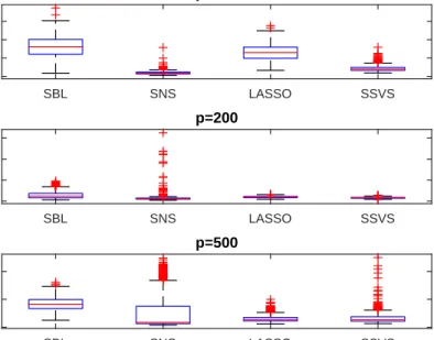
The following Figures 2-4 show boxplots of the MAD statistics for the four algorithms run over the 500 Monte Carlo iterations for the three exercises, respectively. Note first that boxplots of the MAD statistics of a naive, unrestricted estimator (OLS applied using one predictor at a time) is omitted from the three graphs, because these are typically five to 20 times larger

(14)

(depending on the values of T, p) than the MAD values of the four shrinkage algorithms6_{. So} the first general observation is that, even if there are visual differences among the distribution of MAD statistics for the four estimators, these are typically small if the MAD of OLS applied predictor-by-predictor is used as a reference point. WhenT is small relative top, as depicted in Figure 2 for the caseT = 50, the SBL and SNS versions of the GAMP algorithm perform well. On average they give sharper results compared to LASSO and SSVS, with lower averages and more concentrated distributions of MAD statistics. WhenT is larger in which case a different ratio δ is achieved (see discussion in subsection 2.1) then performance of the four algorithms is comparable when p≤T, i.e. for p= 100,200. For the case p= 500 the two GAMP-based algorithms perform slightly worse than the two MCMC-based algorithms, but differences can be considered small (the average MAD of OLS in this case is 0.67, while for the four shrinkage algorithms all average MADs are less than 0.05). In general, under mild correlation among predictors, GAMP-based algorithms perform comparably to MCMC-based algorithms.

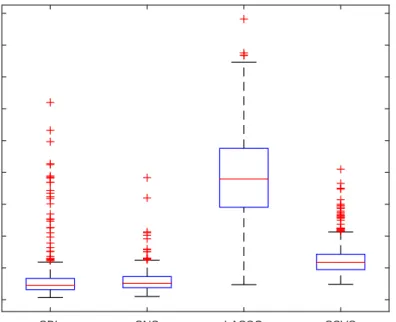
An interesting case is the one where one wants to do inference with correlated predictors. Figure 4 shows what happens in the case T = 200, p = 100. While the assumption p < T seems quite restrictive for general Big Data applications, the example in Model 3 is a quite realistic representation of many modern macroeconomic applications7. In this instance also the performance of GAMP methods is excellent and considerably better than that of the LASSO.

6_{In particular, for the mildly correlated predictors that are generated, the OLS applied predictor-by-predictor} performs as well (in terms of MADs) for the q coefficients which are non-zero. It is for the case of the zero coefficients where the shrinkage estimators generate substantially lower error compared to OLS.

7_{For example, Stock and Watson (2012) and Korobilis (2013) consider datasets with around} _p _{= 100} predictors andT= 200 quarterly observations.

(15)

SBL SNS LASSO SSVS 0 0.02 0.04 p=100 SBL SNS LASSO SSVS 0 0.05 0.1 p=200 SBL SNS LASSO SSVS 0 0.05 0.1 p=500

Figure 2: Boxplots of MAD statistics over the 500 Monte Carlo iterations for Model 1 case (T = 50,p= 100,200,500). SBL SNS LASSO SSVS 0 0.02 0.04 0.06 p=100 SBL SNS LASSO SSVS 0 0.05 0.1 0.15 p=200 SBL SNS LASSO SSVS 0 0.05 0.1 p=500

Figure 3: Boxplots of MAD statistics over the 500 Monte Carlo iterations for Model 2 case (T = 200, p= 100,200,500).

(16)

SBL SNS LASSO SSVS 0 0.02 0.04 0.06 0.08 0.1 0.12 0.14 0.16 0.18

Figure 4: Boxplots of MAD statistics over the 500 Monte Carlo iterations for Model 3 case (T = 200, p= 100).

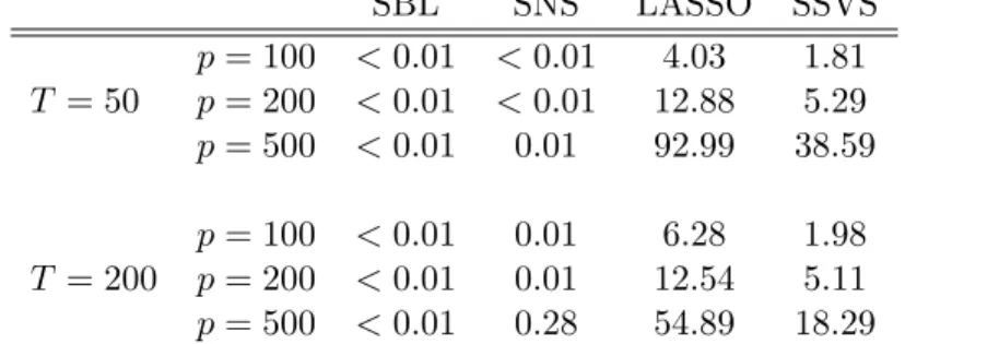
Having established that GAMP-based methods perform comparably when the data generating process is that of a sparse regression model, I proceed to documenting the vast computational gains from the GAMP approximations. Table 1 demonstrates a striking feature of GAMP, that is, the fact that it is much faster than both MCMC-based algorithms used in the simulations above. Entries in this Table are computing times measured in seconds (using the ticand toc commands in MATLAB). The differences are vast, since for the majority of the experiments the GAMP-based algorithms remain below 0.01 seconds. The only exception is for SNS when T = 200 and p = 500, and the explanation is that these algorithms run until a convergence criterion is achieved (as is the case for e.g. the EM algorithm) and in this case convergence took longer. In contrast, MCMC based algorithms have to run for a fixed number of iterations 8. Finally, note that while the GAMP algorithm can be further

8

Note that for the purposes of the Monte Carlo exercise in particular, I run both MCMC-based estimators using only 2000 iterations after discarding an initial 1000 burn-in iterations. This low number ensures satisfactory numerical precision, but in practical situations one would want to run thousand times more MCMC iterations. Thus, the high computing times of LASSO and SSVS are actually favourable due to the limited number of iterations.

(17)

enhanced by trivially modifying it to run in multiple CPU cores, MCMC-based algorithms are not parallelizable unless further approximations are introduced.

Table 1: Computing time (seconds) per Monte Carlo iteration for each of the four algorithms. SBL SNS LASSO SSVS p= 100 <0.01 <0.01 4.03 1.81 T = 50 p= 200 <0.01 <0.01 12.88 5.29 p= 500 <0.01 0.01 92.99 38.59 p= 100 <0.01 0.01 6.28 1.98 T = 200 p= 200 <0.01 0.01 12.54 5.11 p= 500 <0.01 0.28 54.89 18.29

Notes: The reference machine is a 64 bit Windows 7-based PC with Intel Core 7 4770K CPU, 32GB DDR3 RAM running MATLAB 2016a.

4 Empirics

4.1 Forecasting model, data, and competing methods

For the purposes of forecasting, the regression in equation (2) is converted into a forecasting relationship for y by determining appropriately the timing of the predictors. Therefore, the following regression is defined

yt+h =ytφ+Ptβ+εt+h, (21) whereyt+h is theh-step ahead value of the variable of interest andPtare orthogonal predictors, which, following Stock and Watson (2012), are going to be factors from a large macroeconomic dataset. The dataset consists of 222 quarterly U.S. macroeconomic and financial time series observed for the period 1959Q1 - 2015Q3. The series are transformed by taking logarithms and/or differencing, that is, first differences of logarithms are used for real quantity variables, first differences are used for nominal interest rates, and second differences of logarithms for price series. When a given variable is the variable to be predicted, yh_t₊_h, then relevant h-step ahead transformations are defined, see also Stock and Watson (2012) for more details.

All 222 macroeconomic variables are used, one at a time, as the variable of interest, that is, the variable to forecast. The remaining variables are used as exogenous right-hand side

(18)

predictors. In particular, when a high-level aggregate and a subaggregate variable are present, and when these two are typically related by an identity, I only use the lower-level subaggregate to extract factors. This leaves 130 variables to extract the factors from, despite the fact that we evaluate forecasts of all 222 variables. Out of a maximum of 130 factors, I follow Stock and Watson (2012) and use a maximum of 50 factors estimated by simple principal component analysis.

The reqression in equation (21) is estimated using several competing estimators. I contrast the two GAMP-based shrinkage estimators, SBL and SNSdescribed in subsection 2.3, with the following cases

1. Bayesian lasso prior estimated with MCMC (LASSO): More description of this prior and its settings is provided in the previous section and the Technical Appendix.

2. Stochastic search variable selection (SSVS): More description of this prior and its settings is provided in the previous section and the Technical Appendix.

3. Bayesian Model Averaging (BMA): This setting follows Fernandez, Ley and Steel (2001a,b). A g-prior is specified with g = 1/p2, where p is the number of predictors. Estimation is via MCMC methods and in particular the MC3 algorithm of Madigan and York (1995).

4. Bootstrap aggregation or bagging (BAG): Bagging involves generating a large number of bootstrap samples from the original data, calculating least squares estimates, conducting two-sided t-tests on each parameter estimate, generating forecasts and averaging forecasts across bootstrap samples. The exact settings and critical values used are identical to the ones proposed in Ribeiro (2016, pages 6-7).

5. Five factors (DFM5): The DFM-5 forecast uses the first five principle components as predictors, with coefficients estimated by OLS without shrinkage. This is a parsimonious specification and can be thought of as a naive approach to shrinkage that, in practice, may perform better than the state-of-the-art methods outlined above.

(19)

6. Full model (OLS): As an indication of how well shrinkage methods perform, I quote results from the model with all 50 factors included estimated with unrestricted least squares.

7. Minimal model (ARp): This is a the model with zero factors and only a single lag of the dependent variable, estimated by OLS. I do not explicitly quote results for this model, rather I use it as a reference point for other methods (i.e. all results are relative to the AR(1) model).

I use the second half of the sample to evaluate forecasts from the regression model using all estimation methods outlined above. The first estimation period is 1959Q1-1985Q4, and I forecast h = 1,2,4 and 8 steps ahead. Estimation and forecasting is recursive, adding each quarter one observation to the initial estimation sample, until the whole sample is exhausted. That is, the last estimation period is 1959Q1 - (2015Q2-h). Additional results based on rolling forecasts are presented in the Appendix. Given that Bayesian and non-Bayesian estimation methods are compared, I focus on point estimation only, following closely Stock and Watson (2012). Results are typically evaluated by taking two standard distance functions of forecast errors, the rectilinear (l1-norm) and Euclidean (l2-norm), leading to the mean absolute forecast error (MAFE) and the root mean square forecast error (RMFSE).

4.2 Main Results

This section presents the main results of this paper for all 222 series and for the case of recursive forecasts. Additional results for rolling forecasts and for selected series are discussed in the next subsection, and additional tables can be found in the Appendix.

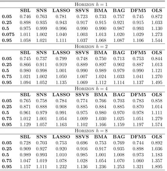
Table 2 reports the distributions of relative root mean squared errors (RMSEs) for the various forecasting methods. The rows represent percentiles of the distribution of RMSEs over the 222 series for the eight forecasting methods, where all RMSEs are relative to the AR(1) benchmark. Values less than one signify improvement over the benchmark, while values larger than one suggest that the benchmark performs well. First note that the general results are

(20)

in-line with the findings of Stock and Watson (2012): All shrinkage or parsimonious methods (that is, excluding OLS using all 50 factors) improve over the AR(1) benchmark. The improvements in some cases are not as large as the ones that Stock and Watson find in their respective Table 2, but note that they use an AR(4) benchmark (which, in general, is inferior to the AR(1) for this kind of data). Additionally, it can also be seen that the forecast improvement from using shrinkage estimators over the naive, but parsimonious, DFM5 approach, is modest. The only consistent pattern that seems to emerge is that in the 95% percentile, the shrinkage methods do not generate as large MSFEs as the DFM5. For example, for h = 8 DFM5 has RMSFE of the order of 32% worse than the benchmark AR(1), while the vast majority of shrinkage estimators provide reduction in forecast accuracy of 10%-20%.

These important observations aside, the main research question in this paper is how GAMP-based algorithms perform compared to other shrinkage algorithms. The answer to that question is strikingly straightforward to respond to based on evidence in Table 2. In particular GAMP-SBL seems to perform extremely well, but also GAMP-SNS follows closely. In terms of the median SBL is better than DFM5 in three out of four forecast horizons, while SNS is performing satisfactorily, meaning that it improves AR(1) forecasts and at the same time is comparable to the performance of the remaining shrinkage methods. In terms of the 5th percentile, all shrinkage methods and the DFM5, are comparable. However, when looking at the 95th percentiles, SBL and SNS generate consistently lower RMSFEs compared to DFM5.

The reason why GAMP-SBL and GAMP-SNS perform consistently well at all forecast horizons, while alternative shrinkage methods might perform well in some cases (e.g. forh= 1) but not so well in others (e.g. for h = 8 all other shrinkage methods, apart from the DFM5, perform worse than the AR(1) in the median), is simply the fact that GAMP-based algorithms do not require tuning of prior quantities, since all hyperpriors are estimated automatically using the EM updates. So when correlations between the predictors and the variable of interest, yt+h, change as the horizonh changes, GAMP-based algorithms will adapt automatically to the new setting. Given the simplicity and tractability of GAMP, one can think of even further enhancements, for example run multiple instances of GAMP using different initial parameter

(21)

guesses in order to eliminate the effect of initial conditions and increase its precision even further. MCMC-based algorithms may also suffer from the effect of initial conditions, but in many cases it may be computationally impractical to run multiple instances of an MCMC algorithm.

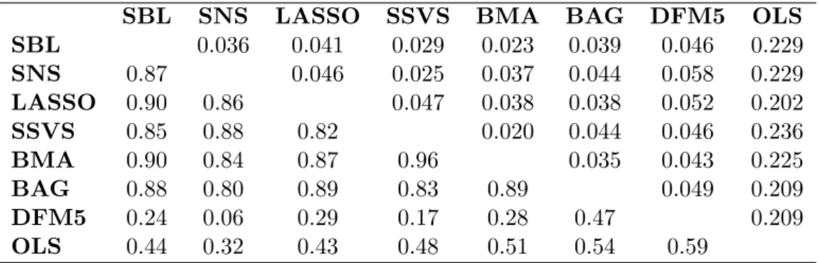
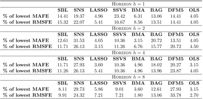
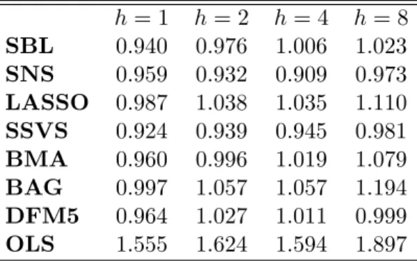
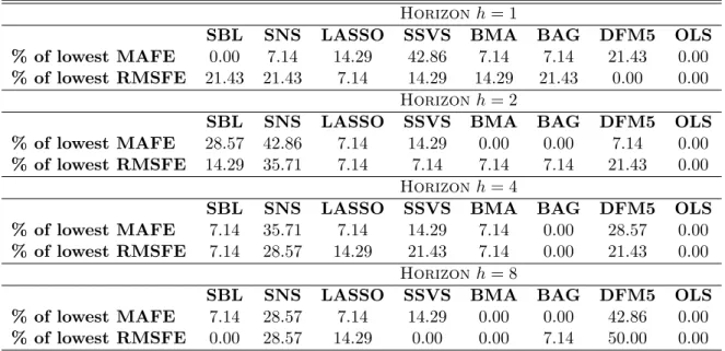
Table 3 summarizes the results of the previous Table by considering the weighted means square forecast error measure (WMSFE) used in Christoffersen and Diebold (1998). This is a weighted measure, where the scale of each of the 222 variables is taken into account. Results are also standardized to be relative to the AR(1) WMSFE. In this table we also see that using this criterion most methods do not perform better than the AR(1), but SBL and SNS are strongly better, especially SBL for h = 3 where improvements are substantial. Table 4 explores whether forecasts from the competing methods differ from each other. Specifically, the Table presents two measures of similarity of the performance of one-step ahead forecasts, namely the correlation (over series) among RMSEs, relative the AR(1) forecasts, and the mean absolute difference of these relative RMSEs. All shrinkage forecasts are highly correlated, while DFM5 and OLS are less correlated with other methods and with each other. Nevertheless, the parsimonious DFM5 generates mean absolute differences which are similar to ones by the shrinkage methods, while the non-parsimonious OLS fails to a large extent to perform well. This suggests two things. First, the two GAMP-based algorithms generate RMSFEs in accordance with other shrinkage methods. Second, even though the first few principal components typically explain most of the variability in a dataset (such as the one used here to extract factors), the shrinkage methods might not be selecting consistently the first few components. If that was the case, their RMSFEs would not have such low correlation with the DFM5 forecasts. This low correlation might suggest that shrinkage methods retain possibly the first few components as well as a mix of less informative components. Finally, Table 5 shows the hit rates in terms of mean absolute and root mean square forecast errors of the eight competing methods. These hit rates simply measure the percentage of times, over the 222 series, that each method had achieved the lowest MAFE or RMSFE. Again, we can see that this criterion also confirms the excellent performance of SBL and particularly SNS compared to all other

(22)

methods. It is noteworthy that the GAMP-based methods retain over all forecast horizons their good percentages of being the best performing methods, while SSVS has gradually decreasing hit-rates while DFM5 consistently improves over the forecast horizons.

Table 2: Distributions of Relative Root Mean Squared Errors (RMSE), Relative to the AR(1) Forecast, by Forecasting Method, all 222 series

Horizon h= 1

SBL SNS LASSO SSVS BMA BAG DFM5 OLS 0.05 0.746 0.763 0.781 0.723 0.733 0.757 0.745 0.872 0.25 0.898 0.935 0.943 0.917 0.915 0.921 0.915 1.033 0.5 0.975 0.999 0.996 0.990 0.990 0.987 0.993 1.130 0.075 1.011 1.002 1.040 1.003 1.013 1.020 1.029 1.273 0.95 1.058 1.021 1.111 1.037 1.068 1.087 1.106 1.544 Horizon h= 2

SBL SNS LASSO SSVS BMA BAG DFM5 OLS 0.05 0.728 0.703 0.753 0.696 0.753 0.769 0.744 0.892 0.25 0.909 0.927 0.920 0.916 0.917 0.935 0.898 1.036 0.5 0.989 0.993 1.010 0.985 1.001 1.008 0.973 1.183 0.75 1.047 1.019 1.078 1.028 1.054 1.070 1.060 1.357 0.95 1.157 1.111 1.232 1.136 1.236 1.253 1.321 1.895

Notes: Entries are percentiles of distributions of relative RMSFEs over the 222 variables being forecasted, by series, at the 1-, 2-, 4- and 8-quarter ahead forecast horizon. RMSFEs are relative to the AR(1) forecast RMSFE, and are computed using an expanding window of in-sample observations (recursive). All forecasts are direct.

(23)

Table 3: Multivariate weighted mean squared forecast error, for each estimator and forecast horizon, all 222 series

h= 1 h= 2 h= 4 h= 8 SBL 0.986 0.980 0.905 0.992 SNS 0.998 0.996 1.032 0.986 LASSO 1.044 1.065 1.106 1.164 SSVS 1.000 1.002 1.076 1.179 BMA 1.034 1.045 1.058 1.133 BAG 1.019 1.046 1.155 0.987 DFM5 0.993 1.077 1.066 1.142 OLS 1.043 1.029 1.126 1.035

Notes: Entries in this table report the multivariate weighted mean squared forecast error of each method relative to the AR(1); see Christoffersen and Diebold (1998) for more details.

Table 4: Two Measures of Similarity of Forecast Performance, h= 1: Correlation (lower left) and Mean Absolute Difference of Forecasts (upper right), all 222 series

SBL SNS LASSO SSVS BMA BAG DFM5 OLS SBL 0.036 0.041 0.029 0.023 0.039 0.046 0.229 SNS 0.87 0.046 0.025 0.037 0.044 0.058 0.229 LASSO 0.90 0.86 0.047 0.038 0.038 0.052 0.202 SSVS 0.85 0.88 0.82 0.020 0.044 0.046 0.236 BMA 0.90 0.84 0.87 0.96 0.035 0.043 0.225 BAG 0.88 0.80 0.89 0.83 0.89 0.049 0.209 DFM5 0.24 0.06 0.29 0.17 0.28 0.47 0.209 OLS 0.44 0.32 0.43 0.48 0.51 0.54 0.59

Notes: Entries below the diagonal are the correlation between the RMSFEs for the row/column forecasting methods, computed over the 222 series being forecasted. Entries above the diagonal are the mean absolute difference between the row/column method RMSFEs, averaged across series.

(24)

Table 5: Hit-rates of the eight estimators, all 222 series

Horizonh= 1

SBL SNS LASSO SSVS BMA BAG DFM5 OLS

% of lowest MAFE 14.41 19.37 4.96 23.42 6.31 13.06 14.41 4.05

% of lowest RMSFE 15.32 22.07 5.41 16.67 8.56 13.51 14.41 4.05

Horizonh= 2

% of lowest MAFE 12.61 31.53 4.05 10.36 3.15 20.72 13.51 4.05

% of lowest RMSFE 11.71 26.13 3.15 11.26 6.76 15.77 20.72 4.50

Horizonh= 4

% of lowest MAFE 11.71 27.93 3.60 10.36 4.96 18.02 20.27 3.15

% of lowest RMSFE 11.26 26.13 5.41 10.36 4.96 13.96 23.87 4.05

Horizonh= 8

% of lowest MAFE 8.11 29.73 5.86 9.01 3.60 12.61 27.93 3.15

% of lowest RMSFE 9.91 24.32 7.21 7.21 1.80 13.06 33.78 2.70

Note: This table shows the proportion of times (over the 222 series being forecasted) that each estimator achieved the lowest value of the MAFE and RMSFE statistics.

4.3 Further results and discussion

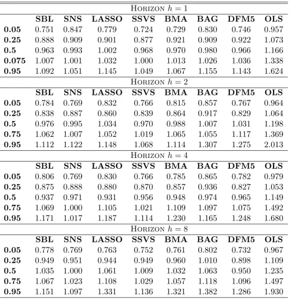
In the Appendix I provide additional results that help solidify the conclusions drawn from the main results. First, I consider the results only on 14 series that are possibly the most important indicators that macroeconomists and analysts look at. These are real GDP, personal consumption expenditures, industrial production (total), employment, unemployment rate, GDP price deflator, consumer price index (total), producer price index (commodities), federal funds rate, 10-year Treasury bond rate, real M1 money stock, GBP/USD exchange rate, and S&P500 stock prices. There are, of course, several leading indicators that one could also follow (hours worked, consumer confidence, mortgage rates etc), nevertheless these 14 series roughly describe the variables of interest (target variables) for policy-makers and central banks. The main argument of doing this exercise is that, when evaluating 222 series, it might be the case that GAMP is performing really well on series which are higher level disaggregates (and possibly not so interesting), while performing poorly on variables that matter. Tables C.1 to

(25)

C4 show that this is not the case.

Qualitatively similar conclusions can be drawn when considering rolling forecasts, that is, forecasts with in-sample estimation of coefficients in a fixed window of observations. Such an approach takes into account evident structural breaks in macroeconomic time series (see Bauwens, Koop, Korobilis and Rombouts, 2015). I follow Stock and Watson (2012) and consider a rolling window of 100 observations, using the same evaluation period for all forecasts. Doing so, means that all shrinkage estimators should “work harder” to find suitable restrictions on regression coefficients and save valuable degrees of freedom, and for that reason parsimonious approaches (the AR(1) and DFM5) are expected to have a possible advantage a-priori. Nevertheless, results are favourable for all shrinkage estimators with SBL and SNS leading the course.

Considering rolling forecasts is a simple approach to control for structural breaks, but choice of the rolling window is subjective. One can consider, instead, specifications that explicitly account for changing volatility, which has been shown to be an extremely important feature of macroeconomic data; see Clark and Ravazzollo (2015). In the Technical Appendix I show different ways to combine the GAMP shrinkage estimators with stochastic volatility. I do not, however, evaluate forecasts from such a specification because it is beyond the scope of this paper, whose focus is on regressions with many predictors. Finally, note that other extensions of GAMP are readily available. In a vector autoregressive (VAR) setting for example, if we consider the decomposition in Carrierro, Clark and Marcellino (2016) that allows for equation-by-equation estimation of the VAR, then application of GAMP is trivial. Similar adaptations to factor models and other popular multivariate specifications are also possible, and they would be an interesting direction for future research in applied econometrics.

5 Conclusions

This paper evaluates a new methodology for performing Bayesian inference in high-dimensional regression models. The proposed Generalized Approximate Message Passing (GAMP) is a

(26)

fast algorithm for approximating iteratively the first two moments of the marginal posterior distribution of high-dimensional coefficients. It is established how effortlessly GAMP can be combined with two popular classes of shrinkage priors, and extensive evaluations in synthetic and real data demonstrate the advantages of using GAMP. In particular, GAMP is at least as precise as a wide class of alternative shrinkage methods, at a fraction of the computing time and with minimal user input. While the kind of application considered in this paper is typical in macroeconomics, it is far from being a truly “Big Data” application. Nevertheless, GAMP will accommodate regression models with thousands or, possibly, millions of predictors before it hits a computational bottleneck. This paper, thus, attempts to make the point that GAMP should become a valuable tool for applied economists and policy-makers who wish to monitor high-dimensional datasets, and that, despite its approximate nature, this fast algorithm is an investment for future generations of macroeconomists who might be faced with a daunting amount of available information to process.

(27)

References

[1] Barber, D. (2012). Bayesian reasoning and machine learning. Cambridge University Press: New York.

[2] Baron, D., Sarvotham, S. and Baraniuk, R. G. (2010). Bayesian compressive sensing via belief propagation.IEEE Transactions in Signal Processing, 58, 269280.

[3] Bauwens, L., Koop, G., Korobilis, D. and Rombouts, J. V. K. (2015). The contribution of structural break models to forecasting macroeconomic series. Journal of Applied Econometrics, 30(4), 596-620.

[4] Bayati, M. and Montanari, A. (2011). The dynamics of message passing on dense graphs, with applications to compressed sensing. IEEE Transactions on Information Theory, 57(2), 764-785.

[5] Breiman, L. (1996). Bagging predictors. Machine learning, 24 (2), 123140.

[6] Carriero, A., Clark, T. E. and Marcellino, M. (2016). Large vector autoregressions with stochastic volatility and flexible priors. Working paper 16-17, Federal Reserve Bank of Cleveland.

[7] Christoffersen, P. and Diebold, F. (1998). Cointegration and long-horizon forecasting.

Journal of Business and Economic Statistics, 16(4), 450-458.

[8] Clark, T. E. (2011). Real-time density forecasts from Bayesian vector autoregressions with stochastic volatility. Journal of Business and Economic Statistics, 29(3), 327-341.

[9] Clark, T. E. and Ravazzolo, F. (2015). Macroeconomic forecasting performance under alternative specifications of timevarying volatility.Journal of Applied Econometrics, 30(4), 551-575.

[10] Donoho, D. L., Maleki, A. and Montanari, A. (2009). Message passing algorithms for compressed sensing.Proceedings of National Academy of Sciences, 106(45), 18914-18919.

(28)

[11] Donoho, D. L., Maleki, A. and Montanari, A. (2011). How to design message passing algorithms for compressed sensing. Unpublished manuscript, available at http://www.ece.rice.edu/ mam15/bpist.pdf.

[12] Fernandez, C., E. Ley, and Steel, M. (2001a). Model uncertainty in cross-country growth regressions.Journal of Applied Econometrics, 16, 563576.

[13] Fernandez, C., E. Ley, and Steel, M. (2001b). Benchmark priors for Bayesian model averaging.Journal of Econometrics, 100, 381427.

[14] Freeman, W. T., Pasztor, E. C., and Carmichael, O. T. (2000). Learning low-level vision.

International Journal of Computer Vision, 40, 2547.

[15] George, E. I. and McCulloch, R. E. (1993). Variable selection via Gibbs sampling.Journal of the American Statistical Association, 88(423), 881-889.

[16] Griffin, J. E. and Brown, P. J. (2010). Inference with normal-gamma prior distributions in regression problems.Bayesian Analysis, 5(1), 171-188.

[17] Ji, S., Xue, Y. and Carin, L. (2008). Bayesian compressive sensing.IEEE Transactions on Signal Processing, 56(6), 2346-2356.

[18] Kamilov, U. S., Rangan, S., Fletcher, A. K. and Unser, M. (2014). Approximate message passing with consistent parameter estimation and applications to sparse learning. IEEE Transactions on Information Theory, 60(5), 2969-2985.

[19] Korobilis, D. (2013). Hierarchical shrinkage priors for dynamic regressions with many predictors.International Journal of Forecasting, 29, 43-59.

[20] Kschischang, F. R., Frey, B. J. and Loeliger, H. A. (2001). Factor graphs and the sum-product algorithm.IEEE Transactions on Information Theory, 47(2), 498-519.

[21] Madigan, D. and York, J. (1995). Bayesian graphical models for discrete data.

(29)

[22] McEliece, R. J., MacKay, D. J. C. and Cheng, J. (1998). Turbo decoding as an instance of Pearls belief propagation algorithm.IEEE Journal on Selected Areas in Communications, 16, 140152.

[23] Park, T. and Casella, G. (2008). The Bayesian lasso. Journal of the American Statistical Association, 103(482), 681-686.

[24] Pearl, J. (1982). Reverend Bayes on inference engines: A distributed hierarchical approach. AAAI-82: Pittsburgh, PA. Second National Conference on Artificial Intelligence. Menlo Park, California: AAAI Press, 133136.

[25] Rangan, S. (2011). Generalized approximate message passing for estimation with random linear mixing.IEEE International Symposium on Information Theory, 2174-2178.

[26] Rangan, S., Schniter, P., Riegler, E., Fletcher, A. K. and Cevher, V. (2016). Fixed points of generalized approximate message passing with arbitrary matrices. arXiv:1301.6295v4 [27] Ribeiro, P. (2016). Revealing Exchange Rate Fundamentals by Bootstrap. Available at

SSRN: https://ssrn.com/abstract=2839259.

[28] Stock, J. H. and Watson, M. W. (2006). Macroeconomic Forecasting Using Many Predictors. Handbook of Economic Forecasting, Graham Elliott, Clive Granger, Allan Timmerman (eds.), North Holland, 2006.

[29] Stock, J. H. and Watson, M. W. (2012). Generalized shrinkage methods for forecasting using many predictors.Journal of Business and Economic Statistics, 30(4), 481-493. [30] Tibshirani, R. (1996). Regression shrinkage and selection via the lasso. Journal of the

Royal Statistical Society, Series B, 58, 267-288.

[31] Vila, J. P. and Schniter, P. (2011). Expectation-maximization Bernoulli-Gaussian approximate message passing. Conference on Signals, Systems, and Computing (ASILOMAR), Pacific Grove, CA, USA, 799-803.

(30)

[32] Vila, J. P. and Schniter, P. (2013). Expectation-maximization gaussian-mixture approximate message passing.IEEE Transactions on Signal Processing, 61(19), 46584672. [33] West, M. and Harrison, P. J. (1997).Bayesian Forecasting and Dynamic Models (2nd ed.).

Springer: New York.

[34] Ziniel, J. and Schniter, P. (2013). Dynamic compressive sensing of time-varying signals via approximate message passing.IEEE Transactions on Signal Processing, 61(21), 5270-5284.

[35] Ziniel, J., Potter, C. and Schniter, P. (2010). Tracking and smoothing of time-varying sparse signals via approximate belief propagation. Procedures of Forty-fouth Asilomar Conference on Signals, Systems, and Computers, Pacific Grove, CA.

[36] Zou, X., Li, F., Fang, J. and Li, H. (2016). Computationally efficient sparse Bayesian learning via generalized approximate message passing. IEEE International Conference on Ubiquitous Wireless Broadband (ICUWB), 1-4.

(31)

A

Data

App

endix

All series w ere do wnloaded from Mic hael McCrac k en’s FRED-QD database (h ttps://researc h.stlouisfed.org/econ/mccrac k en/fred-databases/) in Marc h 2017 and co v e r the quarters 1959Q1 to 2015Q3. Ou t of the original 257 series, on ly 222 ha v e b een retained in order to ensure a balanced panel of observ ations. All series are seasonally adjusted and all v ariables are transformed to b e appro ximately stationary and the transformation co des for eac h v ariable app ear in the column ‘T’ on the table b elo w. In particular, if wi,t is the original un-transformed series in lev els, when the series is used as a predictor via factors (R.H.S. of the regression mo del) the tran sf ormation co des are: 1 -no transformation (lev els), xi,t = wi,t ; 2 -first d iffe rence, xi,t = wi,t − wi,t − 1 ; 3-second difference, xi,t = ∆ wi,t − ∆ wi,t − 1 4 -logarithm, xi,t = log wi,t ; 5 -first difference of logarithm, xi,t = log wi,t − log wi,t − 1 ; 6 -second difference of logarithm, xi,t = ∆ log wi,t − ∆ log wi,t − 1 . When the series is used as the v ariable to b e predicted (L. H.S. of the regression mo del) the transformation co des are: 1 -no transformation (lev els), yi,t + h = wi,t + h ; 2 -first difference, yi,t + h = wi,t + h − wi,t ; 3-second difference, yi,t + h = 1 ∆ h h w i,t + h − ∆ wi,t 4 -logarithm, yi,t + h = log wi,t + h ; 5 -first difference of logarithm, yi,t + h = log wi,t + h − log wi,t ; 6 -second d iffe rence of logarithm, yi,t + h = 1 ∆h h log wi,t + h − ∆ log wi,t . In the transformations ab o v e, I define ∆ wt = wt − wt − 1 and ∆ h w t + h = wt + h − wt . F rom the 222 series, 92 are higher lev e l aggregates and do not add information when extracting p rincipal c omp onen ts . These series are indicated with a 0 in column ‘F ’ of the table b e lo w, and only th e remaining 130 se ri e s are used for extracting factors. T able A 1: Quarterly US macro dataset (based on FREDQD) No Mnemonic F T Long description 1 GDPC96 0 5 Real Gross Domes tic Pro duct, 3 Decimal (Billions of Chained 2009 Doll ar s) 2 PCECC96 0 5 Consumption Real P ersonal Consumption Exp enditures (Billions of Chained 2009 D ollars) 3 PCDGx 1 5 Real p ersonal consumption exp enditures: Durable go o ds (Billi ons of Chained 2009 Dollars), deflated usin g PCE 4 PCESVx 1 5 Real P ersonal Consumption Exp enditures: Services (Billions of 2009 Dollars), deflated using PCE 5 PCNDx 1 5 Real P ersonal Consumption Exp enditures: Nondurable Go o ds (Billions of 2009 Dollars), deflated using PCE 6 GPDIC96 0 5 Real Gross Priv ate Domestic In v estm en t, 3 decimal (Billions of Chained 2009 Dollars) 7 FPIx 0 5 Real priv ate fixed in v est men t (Billions of Chained 2009 D ollars), deflated using PCE 8 Y033R C1Q027SBEAx 1 5 Real G ross Priv ate Domestic Fi xed In v estmen t: Nonresiden tial: Equipmen t (Bi llions of Chained 2009 Dollars), deflated using PCE 9 PNFIx 1 5 Real priv ate fixed in v estmen t: Nonresiden tial (Bill ions of Chained 2009 Dollars), deflated using PCE 10 PRFIx 1 5 Real priv ate fixed in v estmen t: Residen tial (Billi ons of Chained 2009 Dollars), deflated usin g PCE 11 A014RE1Q156NBEA 1 1 In v en tories Shares of gross domestic pro duct: Gross priv ate domest ic in v estmen t: Change in priv ate in v en tories (P ercen t) 12 GCEC96 0 5 R eal Go v ernmen t Cons u m p t ion Exp enditures & Gross In v estme n t (Billions of Chained 2009 Dollars) 13 A823RL1Q225SBEA 1 1 Real Go v ernmen t Consumption Exp enditures and Gross In v estmen t: F ederal (P ercen t Change from Preceding P erio d) 14 F GRECPTx 1 5 Real F ederal Go v ernmen t Curren t Receipts (Billions of Chained 2009 Doll ar s), deflated using PCE 15 SLCEx 1 5 Real go v ernmen t state and lo cal consumption exp enditures (Billions of Chained 2009 Dollars), deflated using PCE 16 EXPGSC96 1 5 Real Exp orts of G o o ds & Services, 3 Decimal (Billions of Chained 2009 Doll ar s) 17 IMPGSC96 1 5 Real Imp orts of Go o ds & Services, 3 Decimal (Billions of Chai ned 2009 Dollars) 18 DPIC96 0 5 Real Disp osable P ersonal Income (Billions of Chained 2009 Dollars) 19 OUTNFB 0 5 Real Disp osable P ersonal Income (Billions of Chained 2009 Dollars) 20 OUTBS 0 5 Business Sector: Real Output (Index 2009=100) 21 INDPR O 0 5 Industrial Pro duction Index (Index 2012=100) 22 IPFINAL 0 5 Industrial Pro duction: Final Pro ducts (Mark et Group) (Index 2012=100) 23 IPCONGD 0 5 Industrial Pro duction: Consumer Go o ds (Index 2012=100) 24 IPMA T 0 5 Industrial Pro duction: Materials (Index 2012=100) 25 IPDMA T 1 5 In dus trial Pro duction: Durable Materials (Index 2012=100) 26 IPNMA T 1 5 Industrial Pro duction: Nondurable Materials (Index 2012=100) 27 IPDCONGD 1 5 Industrial Pro duction: Durable Consumer Go o ds (Index 2012=100) 28 IPB51110SQ 1 5 Industrial Pro duction: Durable Go o ds: Automotiv e pro ducts (Index 2012=100)

(32)

T able A1 (con tin ued) 29 IPNCONGD 1 5 Industrial Pro duction: Du r abl e Go o ds: Automotiv e p r o ducts (Index 2012=100) 30 IPBUSEQ 1 5 Industrial Pro duction: Business Equipmen t (Index 2012=100) 31 IPB51220SQ 1 5 Industrial Pro duction: Cons u m er energy pro ducts (Index 2012=100) 32 CUMFNS 1 1 Capacit y Utilization: Man ufacturing (SIC) (P ercen t of Capacit y) 33 P A YEMS 0 5 A ll Emplo y ees: T otal nonfarm (Thousands of P ers ons) 34 USPRIV 0 5 All Emplo y ees: T otal Priv ate Industries (Thousands of P ersons) 35 MANEMP 0 5 All Emplo y ees: Man ufactur ing (Thousands of P ersons) 36 SR VPRD 0 5 All Emplo y ees: Service-Pro vi ding Industries (Thousands of P ersons) 37 USGOOD 0 5 All Emplo y ees: Go o ds-Pro ducing Industries (Thousands of P ersons) 38 DMANEMP 1 5 All Emplo y ees: Durable go o ds (Thousands of P ersons) 39 NDMANEMP 0 5 All Emplo y ees: Nondurable go o ds (Thousands of P ersons) 40 USCONS 1 5 All Emplo y ees: Construction (T housands of P ersons) 41 USEHS 1 5 All Emplo y ees: Education & Health Services (Thousands of P ersons) 42 USFIRE 1 5 All Emplo y ees: Education & Health Services (Thousands of P ersons) 43 USINF O 1 5 All Emplo y ees: Inf ormation Services (Thousands of P ers on s ) 44 USPBS 1 5 All Emplo y ees: Professional & Business Services (Thousands of P ersons) 45 USLAH 1 5 All Emplo y ees: Leisure & Hospitalit y (Thousands of P ersons) 46 USSER V 1 5 Al l Emplo y ees: Other Services (Thousands of P ersons) 47 USMINE 1 5 All Emplo y ees: Mining and logging (Thousands of P ersons) 48 USTPU 1 5 All Emplo y ees: T rade, T ransp ortation & Utilities (Thousands of P ersons) 49 USGO VT 0 5 All Emplo y ees: Go v ernmen t (Thousands of P ersons) 50 USTRADE 1 5 All Emplo y ees: Retail T rade (Thousands of P ersons) 51 USWTRADE 1 5 All Emplo y ees: Wholesale T rade (Thousands of P ersons) 52 CES9091000001 1 5 All Emplo y ees: Go v ernmen t: F ederal (Thousands of P ersons) 53 CES9092000001 1 5 All Emplo y ees: Go v ernmen t: State Go v ernmen t (Thousands of P ersons) 54 CES9093000001 1 5 All Emplo y ees: Go v ernmen t: Lo cal Go v ernmen t (Thousands of P ersons) 55 CE16O V 0 5 Civilian Emplo ymen t (Thousands of P ers on s ) 56 CIVP AR T 0 2 Civilian Lab or F orce P articipation Rate (P ercen t) 57 UNRA TE 0 2 Civilian Unemplo ymen t Rate (P ercen t) 58 UNRA TESTx 0 2 Unemplo ymen t Rate less than 27 w eeks (P ercen t ) 59 UNRA TEL T x 0 2 Unemplo ymen t Rate for more than 27 w eeks (P ercen t) 60 LNS14000012 1 2 Unemplo ymen t Rate -16 to 19 y ears (P ercen t) 61 LNS14000025 1 2 Unemplo ymen t Rate -20 y ears and o v er, Men (P ercen t) 62 LNS14000026 1 2 Unemplo ymen t Rate -20 y ears and o v er, W omen (P ercen t) 63 UEMPL T5 1 5 N u m b er of Civilians Unem p lo y ed -Less Than 5 W eeks (Thousands of P ersons) 64 UEMP5TO14 1 5 Num b er of Civilians Unemplo y ed for 5 to 14 W eeks (Thous an ds of P ersons) 65 UEMP15T26 1 5 Num b er of Civilians Unemplo y ed for 15 to 26 W eeks (Thousands of P ersons) 66 UEMP27O V 1 5 Num b er of Civilians Unemplo y ed for 27 W eeks and Ov er (Thousands of P ersons) 67 LNS12032194 1 5 Emplo ymen t Lev el -P art-Time for Econ om ic Reasons, All Industr ies (Thousands of P ersons) 68 HO ABS 0 5 Business Sector: Hours of All P er sons (Index 2009=100) 69 HO ANBS 0 5 Nonfarm Business Sector: Hours of All P ersons (Index 2009=100) 70 A WHMAN 1 1 Av erage W eekly Hours of Pro duction and Nonsup ervisory Emplo y ees: Man ufacturing (Hours) 71 A W OTMAN 1 2 Av erage W eekly Hours Of Pro duction And Nonsup ervisory Emplo y ees: T otal priv ate (Hours) 72 HWIx 0 1 Help-W an ted Index 73 HOUST 0 5 Housing Starts: T otal: New Priv ately Owned Housing Units Started (Thousands of Units) 74 HOUST5F 0 5 Housing Starts: T otal: New Priv ately Owned Housin g Units Started (Thousands of Units) 75 PERMIT 1 5 New Priv at e Housing Units Authorized b y Build ing P ermits (Thousands of Units) 76 HOUSTMW 1 5 H ou s ing Starts in Mi dw est Census Region (Thousands of Units) 77 HOUSTNE 1 5 Housing Starts in Northeast Census Region (Thous an ds of Units) 78 HOUSTS 1 5 Housing Starts in South Census Region (Thousands of Units) 79 HOUSTW 1 5 Housing Starts in W est Census Region (Thousands of Units) 80 CMRMTSPLx 0 5 Real Man ufacturing and T rade Industries Sales (Millions of Chained 2009 Dollars) 81 RSAFSx 1 5 Real Retail and F o o d Services Sales (Mill ions of Chained 2009 Dollars), deflated b y Core PCE 82 AMDMNOx 1 5 Real Man ufacturers New Orders: Durable Go o ds (Millions of 2009 Dollars), deflated b y Core PCE 83 AMDMUOx 1 5 Real Man ufacturers Unfilled Orders for Durable Go o ds (Million of 2009 Dollars), deflated b y Core PC E 84 NAPMSDI 1 1 ISM Man ufacturing: Supplier Deliv eries Index (lin) 85 PCECTPI 0 6 P ersonal Consumption Exp enditures: Chain-t yp e Price Index (Index 2009=100) 86 PCEPILFE 0 6 P ersonal Consumption Exp enditures Excluding F o o d and Energy (Index 2009=100) 87 GDPCTPI 0 6 Gross Domestic Pro duct: Chain-t yp e Price Index (Index 2009=100) 88 GPDICTPI 1 6 Gross Priv ate Domestic In v estmen t: Chain-t yp e Price Index (Index 2009=100) 89 IPDBS 1 6 Business Sector: Implicit Price Deflator (Index 2009=100)

(33)

T able A1 (con tin ued) 90 DGDSR G3Q086SBEA 0 6 Go o ds P ersonal consumption exp enditures: G o o ds (c h ain-t yp e price index) 91 DDURR G3Q086SBEA 0 6 P ersonal consumption exp enditures: Durable go o ds (c hain-t yp e price index) 92 DSERR G3Q086SBEA 0 6 P ersonal consumption exp enditures: Services (c hain-t yp e price index) 93 DNDGR G3Q086SBEA 0 6 P ersonal consumption exp enditures: Nondurable go o ds (c hai n-t yp e price index) 94 DHCER G3Q086SBEA 0 6 P ersonal consumption e x p enditures: Nondurable go o ds (c hain-t yp e price index) 95 DMOTR G3Q086SBEA 1 6 P ersonal consumption exp enditures: Durable go o ds: Motor v ehicles and parts (c hain-t yp e price index) 96 DFDHR G3Q086SBEA 1 6 P ersonal consumption exp enditures: Durable go o ds: F urnishings and durable household equipmen t (c hain-t yp e price index) 97 DREQR G3Q086SBEA 1 6 P ersonal consumption exp enditures: Durabl e go o ds: Recreational go o ds and v ehicles (c hain-t yp e price index) 98 DODGR G3Q086SBEA 1 6 P ersonal consumption exp enditures: Durable go o ds: Other durable go o ds (c hain-t yp e price index) 99 DFXAR G3Q086SBEA 1 6 P ersonal consumption exp enditures: Nondurable go o ds: F o o d and b ev er ages purc hased for off-premises consumption (c hain-t yp e price index) 100 DCLOR G 3Q086SBEA 1 6 P ersonal consumption exp enditures: Nondurable go o ds: Clothing and fo ot w ear (c hain-t yp e price index) 101 DGOER G 3Q086SBEA 1 6 P ersonal cons u m p t ion exp enditures: Nondurable go o ds: Gasoline and other energy go o ds (c hain-t yp e price index) 102 DONGR G3Q086SBEA 1 6 P ersonal consumption exp enditures: Nondurable go o ds: Other nondurable go o ds (c hain-t yp e price index) 103 DHUTR G 3Q086SBEA 1 6 P ersonal consumption exp enditures: Services: Housing and utilities (c hain-t yp e price index) 104 DHLCR G 3Q086SBEA 1 6 P ersonal cons u m p t ion exp enditures: Services: Health care (c hain-t yp e price in dex) 105 DTRSR G3Q086SBEA 1 6 P ersonal consumption exp enditures: T ransp ortation services (c hain-t yp e price index) 106 DR CAR G3Q086SBEA 1 6 P ersonal consumption exp enditures: Recreation services (c hain-t yp e price index) 107 DFSAR G3Q086SBEA 1 6 P ersonal consumption exp enditures: Services: F o o d services and accommo dations (c hai n-t yp e price index) 108 DIFSR G3Q086SBEA 1 6 P ersonal consumption exp enditures: Financial se rvi ces and insurance (c hain-t yp e price index) 109 DOTSR G 3Q086SBEA 1 6 P ersonal consumption exp enditures: Other services (c hain-t yp e price index) 110 CPIA UCSL 0 6 C onsumer Price Index for All Urban Consumers: All Items (Index 1982-84=100) 111 CPILFESL 0 6 Consumer Price Index for All Urban Consumers: All Items Les s F o o d & Energy (Index 1982-84=100) 112 PPIF G S 0 6 Pro ducer Price Index b y Commo dit y for Finished Go o ds (Index 1982=100) 113 PPIA C O 0 6 Pro du c er Price Index for All Commo dities (Index 1982=100) 114 PPIF C G 1 6 Pro ducer Price Ind e x b y Commo dit y for Finished Consumer Go o ds (Index 1982=100) 115 PPIF C F 1 6 Pro ducer Price Index b y Commo dit y for Finished Consumer F o o ds (Index 1982=100) 116 PPI IDC 1 6 Pro ducer Price Index b y Commo dit y Industrial Commo dities (Index 1982=100) 117 PPI ITM 1 6 Pro ducer Price Index b y Commo dit y In termediate Materials: Supplies & C omp onen ts (Index 1982=100) 118 NAPMPRI 1 1 ISM Man ufacturing: Prices Index (Index) 119 WPU0561 1 5 Pro ducer Price Index b y Commo dit y for F uels and Related Pro ducts and P o w er: Crude P etroleum (Domestic Pro duction) (Index 1982=100) 120 OILPRICEx 0 5 Real Crude Oil Prices: W est T exas In termediate ( WTI) -Cushing, Oklahoma (2009 Dollars p er Barrel), deflated b y Core PCE 121 CES2000000008x 0 5 Real Av erage Hourly Earnings of Pro duction and Nonsup ervisory Emplo y ees: Construction (2009 Dollars p er Hour), deflated b y Core PCE 122 CES3000000008x 0 5 Real Av erage Hourly Earnings of Pro duction and Nonsup ervisory Emplo y ees: M an ufacturing (2009 Doll ar s p er Hour), deflated b y Core PCE 123 COMPRNFB 1 5 Man ufacturing Sector: Real Comp ensation P er Hour (Index 2009=100) 124 R CPHBS 1 5 Business Sector: Real Comp ensation P er Hour (Index 2009=100) 125 OPHNFB 1 5 Nonfarm Business Sector: Real Output P er Hour of All P ersons (Index 2009=100) 126 OPHPBS 0 5 Business Sector: Real Output P er Hour of All P ersons (Index 2009=100) 127 ULCBS 0 5 Business Sector: Unit Lab or Cost (Index 2009=100) 128 ULCNFB 1 5 Nonfarm Busi nes s Sector: Unit Lab or Cost (Index 2009=100) 129 UNLPNBS 1 5 Nonfarm Business Sector: Unit Nonlab or P a ymen ts (Index 2009=100) 130 FEDFUNDS 1 2 Effectiv e F ederal F un ds Rate (P ercen t) 131 TB3MS 1 2 3-Mon th T reasur y Bill: Secondary Mark et Rate (P ercen t) 132 TB6MS 0 2 6-Mon th T reasur y Bill: Secondary Mark et Rate (P ercen t) 133 GS1 0 2 1-Y ear T reasury Cons tan t Maturit y Rate (P ercen t) 134 GS10 0 2 10-Y ear T reasury Constan t Maturit y Rate (P ercen t) 135 AAA 0 2 Mo o dys Seasoned Aaa Corp orate Bond Yield (P ercen t) 136 BAA 0 2 Mo o dys Seasoned Baa Corp orate Bond Yield (P ercen t) 137 BAA10YM 1 1 Mo o dys Seasoned Baa Corp orate Bond Yield Relativ e to Yield on 10-Y ear T reas ury Constan t Maturit y (P ercen t) 138 TB6M3Mx 1 1 6-Mon th T reasury Bill Min us 3-Mon th T reasury Bil l, secondary mark et (P ercen t) 139 GS1TB3Mx 1 1 1-Y ear T reasury Constan t Maturit y Min us 3-Mon th T reasury Bill, secondary mark et (P ercen t) 140 GS10TB3Mx 1 1 10-Y ear T reasury Constan t Maturit y Min us 3-Mon th T reasury Bill, secondary mark et (P ercen t) 141 CPF3MTB3Mx 1 1 3-Mon th Commercial P ap er Min us 3-Mon th T reasury Bill, secondary mark et (P ercen t) 142 AMBSLREALx 1 5 St. Louis Adjusted Monetary Base (Billions of 1982-84 Dollars), deflated b y CPI 143 M1REALx 1 5 R eal M1 Money Sto c k (Billions of 1982-84 Dollars), deflated b y CPI 144 M2REALx 1 5 R eal M2 Money Sto c k (Billions of 1982-84 Dollars), deflated b y CPI 145 MZMREALx 1 5 Real MZM Money Sto c k (Billions of 1982-84 Dollars), deflated b y CPI 146 BUSLO AN S x 1 5 Real Commercial and Industrial Loans, All Commercial Banks (Billions of 2009 U.S. Dollars), deflated b y Core PCE 147 CONSUMERx 1 5 Consumer Loans at All Commercial Banks (Billi ons of 2009 U.S. Dollars), deflated b y Core PCE 148 NONREVSLx 1 5 T otal Real Nonrev olving Credit Owned and Securitized, Outstanding (Bill ions of Dollars), deflated b y Core PCE 149 REALLNx 1 5 Real Real-Estate Loans, All Commercial Banks (Billions of 2009 U.S. Dollars), deflated b y Core PCE 150 TOT ALSLx 1 5 T otal Consumer Credit Outstanding, deflated b y Core PCE