A GNSS-R Geophysical Model Function: Machine
Learning for Wind Speed Retrievals
Milad Asgarimehr , Irina Zhelavskaya, Giuseppe Foti , Sebastian Reich , and Jens Wickert
Abstract— A machine learning technique is implemented for retrieving space-borne Global Navigation Satellite System Reflec-tometry (GNSS-R) wind speed. Conventional approaches com-monly fit a function in a predefined form to matchup data in a least-squares (LS) sense, mapping GNSS-R observations to wind speed. In this study, a feedforward neural network is trained for TechDemoSat-1 (TDS-1) wind speed inversion. The input variables, along with the derived bistatic radar cross-sectionσ0, are selected after investigating the wind speed dependence and the model performance. When compared to an LS-based approach, the derived model shows a significant improvement of 20% in the root mean square error (RMSE). The proposed neural network demonstrates an ability to model a variety of effects degrading the retrieval accuracy such as the different levels of the effective isotropic radiated power (EIRP) of GPS satellites. For example, the derived Mean Absolute Error (MAE) of the satellite with SVN 34 is decreased by 32% using the machine-learning-based approach.
Index Terms— Geophysical model function (GMF), Global Navigation Satellite System Reflectometry (GNSS-R), machine learning, neural networks, TechDemoSat-1 (TDS-1), wind speed.
I. INTRODUCTION
G
NSS forward scatterometry, as a relatively new Earth observation technique, provides surface-wind informa-tion and, therefore, adds important informainforma-tion to the global state of the atmosphere. The Global Navigation Satellite System Reflectometry (GNSS-R) receivers onboard low Earth orbit satellites, such as TechDemoSat-1 (TDS-1) and CYclone GNSS (CYGNSS), produce a 2-D map of the diffuse scattered power of GPS signal as a function of time delay and Doppler frequency shift, which is known as the delay-Doppler map (DDM). The translation of the bistatic radar cross section, which in turn is a function of the ocean roughness, to the DDM is explained by the bistatic radar equation (BRE) [1]. TheManuscript received July 25, 2019; accepted October 17, 2019. This work was supported by Geo.X, the Research Network for Geosciences in Berlin and Potsdam.(Corresponding author: Milad Asgarimehr.)
M. Asgarimehr and J. Wickert are with the Institute of Geodesy and Geoinformation Science, Faculty VI, Technische Universität Berlin, 10623 Berlin, Germany, and also with the German Research Center for Geosciences GFZ, 14473 Potsdam, Germany (e-mail: [email protected]; [email protected]).
I. Zhelavskaya is with the Institute of Physics and Astronomy, Univer-sity of Potsdam, 14469 Potsdam, Germany, and also with the German Research Center for Geosciences GFZ, 14473 Potsdam, Germany (e-mail: [email protected]).
G. Foti is with the National Oceanography Center, Southampton SO14 3ZH, U.K. (e-mail: [email protected]).
S. Reich is with the Department of Mathematics, University of Potsdam, 14469 Potsdam, Germany (e-mail: [email protected]).
Color versions of one or more of the figures in this letter are available online at http://ieeexplore.ieee.org.
Digital Object Identifier 10.1109/LGRS.2019.2948566
inverse conversion, retrieving wind speed from GNSS obser-vations, can be carried out using a forward operator mapping the observable to wind speed, usually derived in an empirical sense. In literature, this operator is called geophysical model function (GMF).
To fit an accurate GMF to the full range of wind speeds, uniform quality input data or, at least, input data with known error properties, are needed. Generally, it is not easy to meet this condition. Given the limited coverage of the available data, the derived GMF may be degraded in regions where the data coverage is sparse. In the case of determining wind speed GMFs, input data may lack sufficient measurements at high and very low wind speeds. This fact can be problematic when there are strong nonlinearities between the input and the output. Hence, the model-fitting approaches may fail to accurately model the output as a function of the input. Many measurements concentrated on a specific region coupled with data-sparse regions lead to nonuniform GMF performance. As a result, the wind speed retrievals relying on approaches fitting the observables from measured DDMs to a matchup data set, usually in an LS sense, may not have a uniform accuracy within the entire wind speed range. On the other hand, LS-based approaches are commonly used in numerous studies retrieving either state of the ocean or directly the wind speed (see e.g., [2]–[5].)
Moreover, conventional fittings use a predetermined form of function. Any potential disagreements between the true and the predefined functions can introduce an additional bias to the final retrieval. In addition to the unknown validity of the predefined form, ignored factors affecting GNSS-R observations may introduce further inaccuracies. These effects can be either geophysical, such as those from nonwind-derived waves [6] and precipitation [7], or nongeophysical effects such as differences in the level of the GNSS transmitted power. Various manufacturers have built GPS satellites in distinct blocks with different signal levels and differences in the angular distribution of the gain [8]. In addition, the EIRP is not at the same strength for different GPS satellites which are expected to have a higher output power than their end-of-life specification. This fact may cause inaccuracies in the computed TDS-1 bistatic radar cross-section σ0 and, conse-quently, in the obtained ocean wind speeds. Currently, direct incorporation of the transmitting signal levels in TDS-1 winds is not possible as the information is not available in the current data sets.
Artificial neural network (ANN) is a machine learning tech-nique that is inspired by the structure of the brain [9]. ANNs
1545-598X © 2019 IEEE. Personal use is permitted, but republication/redistribution requires IEEE permission. See http://www.ieee.org/publications_standards/publications/rights/index.html for more information.
(i.e., wind speed here), can be conducted. This procedure may also incorporate the unknown effects and dependencies which are not yet physically revealed. ANNs are a nonparametric approach requiring no predefined form of function. Hence, the inaccuracies associated with an imperfect predefined form of function can be addressed.
ANNs have shown promising performance in sea ice detec-tion from space (see e.g., [11]). They have also been used for extracting wind speed from signals of the BeiDo G4 satellite received at a ground station [12]. Nevertheless, their per-formance being implemented for wind speed retrievals from space-borne DDMs is not yet characterized. In this study, a GMF for TDS-1 measurements, mapping GNSS-R observa-tions to wind speed, based on a feedforward ANN is derived and compared with conventional GMFs based on LS fittings. Section II introduces the data sets used for determining and evaluating the GMFs. Section III describes the ANN training approach, architecture, and input variables. The validation study and comparisons to the LS-based approach is conducted in Section IV. Finally, Section V discusses the results followed by the concluding remarks in Section VI.
II. TRAINING, VALIDATION,ANDTESTDATA
The same data sets and TDS-1 σ0 computation algorithm
are used as in [2]. Training the ANN with the same data set enables us to robustly compare the two methods and avoid a biased analysis. Then, by changing only the GMF, the comparison would reveal the advantages and disadvantages associated with the methods under study and not with the data sets. Nevertheless, the input data and obtaining the TDS-1 cross section are briefly described in this section, while the reader may refer to [2] for further details.
The level 1b TDS-1 data from May 2015 until the end of June 2017 are used. The ice-affected ocean, higher than 55◦ latitude, is excluded from the analyses. The data are available to the users by the Measurement of Earth-Reflected Radionavi-gation Signals By Satellite (MERRByS) [13]. To determine the GMFs for TDS-1 observations, a matchup data set, used as the data for training the ANN and also fitting the function by LS, is required. To this end, TDS-1 measurements are collocated with 6-h reanalysis wind fields of ERA-Interim which is based on the Integrated Forecast System European Center for Medium-Range Weather Forecasts (ECMWF). The reanalysis assimilates data from various sources including satellite and ground-based observations [14]. The collocation is conducted within 60 km and 30 min. Around 87% of randomly selected data, 414 684 measurements, from TDS-1/ERA-Interim mea-surements are used for training the ANN (as training and validation data used in Section III), while the remaining data, 61 846 measurements, are employed for the evaluation and
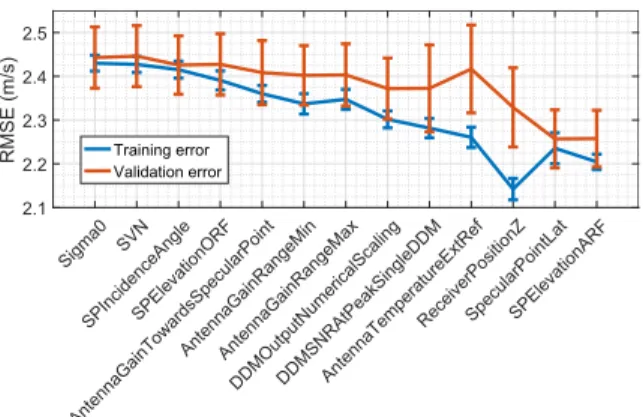
Fig. 1. Successively incorporation of variables and the corresponding RMSEs for the training and validation data.
comparisons, which are never seen by ANN during training procedure (as test data used in Section IV). Bistatic radar cross-section σ0 associated with the peak-received power is obtained using the BRE [1] and as described in [2].
III. DETERMINING THEANN-BASEDGMF Various types of ANNs exist. In this study, the feedforward ANN with one hidden layer is used [15]. One hidden layer is usually sufficient to approximate any continuous function [16]. To train the network, the Levenberg–Marquardt (LM) algo-rithm is implemented, the original description of which is given in [17].
We employ the fivefold cross-validation (CV) procedure [18] with 10 repetitions in order to find the optimal number of neurons in the hidden layer. During the fivefold CV, all available data are split into five chunks of equal size, where one chunk is used for validation and four remaining chunks are used for training. These chunks alternate, so each time the network performance is tested on different data (we can train and test five ANNs in the fivefold CV). That allows us to estimate the generalization ability of a neural network and to obtain the mean and standard deviation of error that can be used to identify whether the network overfits, underfits, or produces reasonable results. We select ANNs with the number of neurons in the hidden layer, which have the minimal error on the validation data.
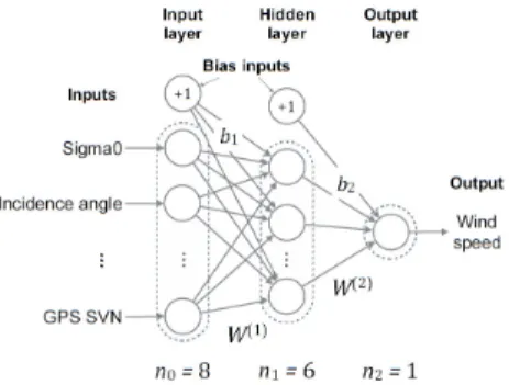
In addition to the computed σ0, L1b TDS-1 data pro-vides a variety of parameters related to either the transmit-ter or receiver satellite and antenna. To collect the optimal set of input variables, those introducing correlations with the wind speed are successively incorporated into the model. In this case, the incorporation results in a reduction of the obtained RMSE on the validation data, and the variable is considered as a further input. Fig. 1 demonstrates how the incorporation of the variables affects the resulting RMSEs of the training and validation data. After testing all variables, eight were selected based on their reduction in RMSE. These are listed in Fig. 2. showing the eventual ANN architecture.
IV. PERFORMANCECHARACTERIZATION
In order to evaluate the proposed machine learning tech-nique and discover its advantages and disadvantages, the pro-posed ANN-based GMF is compared to the retrieval algorithm
Fig. 2. Architecture of the final derived ANN as the inverse GMF. Parameters
n,b, andwindicate the number of neurons in each layer, the bias input, and the weights, respectively. Input variables:σ0in dB, SVN of GPS satellites, specular point (SP) incidence angle in degree, SP elevation in the Orbital Reference Frame (ORF) in degree, Antenna gain toward SP in dB, SP latitude in degree, DDM output numerical scaling in power counts, andZ-component of the receiver in position in Earth-centered, Earth-fixed (ECEF) in meters.
Fig. 3. (a) Wind speed derived from ANN GMF and (b) least-squares-based GMF versus ERA-Interim test observations.
developed in [2] which uses the predefined form of inversion as an exponential function, U10 = Aebσ
0
+C, where the values of A, B, and C are determined by LS. Fig. 3 shows the comparison of TDS-1 derived wind speeds using both approaches. The comparisons are conducted using only test observations (excluded from the training procedure and never seen by ANN before). ANN demonstrates a bias of 0.01 m/s and RMSE of 2.20 m/s, while the LS-based approach results in a bias of −0.16 m/s and RMSE of 2.76 m/s. The ANN reduces the RMSE by 20%.
As shown in Fig. 3, TDS-1 winds overestimate winds lower than 2.5 m/s. This trend is intrinsic and physically explainable. According to the model clarifying the diffuse scattering at low winds [19], the scattering mechanism changes to a higher-order Bragg-like scattering rather than the expected forward quasi-specular mechanism whose magnitude is controlled by the low-pass mean square slope (MSS). The already conducted simulations based on this model, shown in [7], demonstrate how σ0 loses its sensitivity to wind speeds lower than 2.5 m/s. A similar overestimation of low wind conditions is also reported in CYGNSS retrievals [20]. Furthermore, the performance at high wind speeds shows larger biases with a tendency to underestimation. This is also expected as the main observable,σ0, is less sensitive to wind speed change in this region. The underestimation at CYGNSS-derived high winds is also similarly reported [20]. Likewise, radar scatterometers also show a performance degradation at high wind speeds despite the differences in scattering mechanism [21]. It should also be noted that ERA-Interim might have its own deficiencies
Fig. 4. MAE of ANN (red) and LS (blue)-based GMFs versus wind speed (left vertical axis), along with the data histogram in the background (right
vertical axis) .
Fig. 5. MAE of ANN (red) and LS (blue)-based GMFs for each GPS satellite indicated by SVN. The block of each satellite is also reported over the bars.
resolving high and low winds. As a result, the overestimation and underestimation at extreme regimes may be more pro-nounced.
Fig. 4 shows the comparison of the differences between the derived winds from both methods versus ERA-Interim wind speed. Accordingly, ANN-based GMF has a signifi-cantly better performance demonstrating smaller MAE for wind speeds between 2.5 and 10 m/s compared to the LS regression, and as another striking fact, the standard deviation (std) derived from the ANN is significantly smaller in this range of winds. At higher wind speeds, ANN maintains its superiority marginally up to wind speed of 17 m/s. In addition, the MAE of ANN- and LS-based methods are compared versus the Space Vehicle Numbers (SVNs) and other input variables in Figs. 5 and 6, respectively. Fig. 5 demonstrates how the MAE for observations of signals transmitted by different GPS satellites is significantly decreased by the ANN. According to Fig. 6, the MAE is generally decreased by ANN over the input variables.
In addition, Fig. 7 shows the ANN-derived winds in July 2017 which is beyond the training, validation, and test data sets time window. The winds are compared to MERRByS L2 Fast Delivery Inversion (FDI) products [13].
V. DISCUSSION
According to Fig. 1, the ANN model responds to successive incorporation of additional variables as the input along with σ0 demonstrating a continuous reduction in the mean RMSE
of the model. This fact, as well as the smaller std values shown in Fig. 4, is the evidence that there are still unmodeled effects
Fig. 6. (a)–(f) MAE of ANN (red) and LS (blue)-based GMFs on test data versus different input variables.
Fig. 7. (a) Wind speed derived from ANN GMF and (b) L2 FDI products versus ERA-Interim observations in July 2017.
affecting the LS model-fitting. These effects are modeled by ANN resulting in a better performance. The systematic patterns in the data are captured by the ANN as dictated by the data themselves and without a need to direct information. On the other hand, this capability also results in the difficulty of interpreting the physical behavior. This empirical function, in a form of weights, subfunctions, and operators in the architecture of an ANN, could not be described as the way predefined functions are. Nevertheless, possible commentaries can be provided.
The different level of EIRP from the GPS satellites is one of the known factors introducing additional biases in GNSS-R derived winds. According to the International GNSS Service (IGS) models and as shown in [8], Block IIA and IIR satellites have a comparable transmit power of about 50–60 W, respec-tively. However, the discrepancy is much larger in comparison to the IIRM satellites with values of 143–150 W, and even
EIRP values, can be modeled by the ANN capturing the differences from the input SVN and the geometrical features. As a result, a significant improvement in the performance (reduction in MAE value) of GPS satellites, especially the older ones transmitting a lower level of power, is expected as shown in Fig. 5. Accordingly, higher RMSE of SVN 34, the old satellite from block IIA, is shown in Fig. 5 which is decreased as large as 1.2 m/s (≈32%) by ANN.
In addition to IERP and discrepancies between GPS blocks and the gain pattern differences, Blocks IIR-M and IIF redis-tribute transmit power causing a geographical variation in the transmitted power since January 2017 [22]. The documented Flex power during TDS-1 data time span in this study is permanently enabled at 41◦E/37◦N located over land. The global mode is observed on L1 and L2 on four consecutive days in April 2018. As a result, the derived winds can be supposed unaffected in this study.
The LS normally tends to fit the function so that the squared error is minimized, which consequently results in a better performance where most of the data reside in. This can be seen in Fig. 6(a)–(c). According to Fig. 6(a), the majority of data has an incidence angle of 10◦–30◦where the two approaches converge with similar performance. ANN has decreased gen-erally the MAE assisting for correction of errors associated with incidence angle, in computingσ0. At a higher incidence
angle, the values of MAE are statistically insignificant and meaningless as the data in the bins are not sufficient as shown with the histogram in the background. As the power differences are the function of the geometry, a similar trend versus geometry correlated variables, in Fig. 6(b) and (c) are demonstrated, shows higher levels of improvement at low data probabilities. Incorporation of the receiver antenna gain as input into the ANN helps to account for calibration issues and uncertainties related to the derivation of theσ0 from the DDMs. “DDM output numerical scaling” is the scaling applied to the 16-bit DDM variables files. This parameter corresponds to the value of the maximum DDM pixel before scaling for the 16-bit storage range and might help to recover and count for the information lost during this scaling. According to Fig. 6(d), ANN has marginally improved the performance versus DDM output numerical scaling at lower values, and the failure of the technique in modeling the potentially associated effect at higher values, due to the extremely low number of data and insufficient training in this range, is evident. However, the MAE values can be meaningless in this regime due to the insufficient number of data in each bin.
Fig. 6(e) and (f) shows the highest data probability in the southern hemisphere due to the larger ocean area compared to the northern hemisphere. This is exactly where both methods
show similar performance with converging MAEs at latitudes
−45◦–−20◦, due to the LS tendency to minimizing the error where the majority of data reside in. The convergence in performance with the same level of MAE is also observed at latitudes 20◦–45◦, due to the existing symmetries in TDS-1 orbit and GPS constellation with respect to the equator. In the end, ANN has been successful in capturing the differences for reflections in the equatorial regions showing better perfor-mance in this area.
Fig. 7 shows the performance of the ANN beyond the data sets time window in July 2017. The generality of the model is further approved with a similar performance to that on the test data. As the instrument behavior changes, especially in final periods of its operation time, any retrieval model should be recalibrated. This could be why the FDI products also show a severe degradation as TDS-1 approaches its end of mission. Nevertheless, ANN shows more stability compared to traditional approaches. This is due to its modeling nature, multivariable modeling and predicting the modification on σ0 imposed by changes in other input variables.
VI. CONCLUSION
In this study, the implementation of machine learning as an alternative approach for determining a space-borne GNSS-R GMF was investigated. The technique shows promising results in modeling the effects dictated by the data themselves cap-turing the relationships between the input and output based on the found input-output training examples. This fact as well as its nonparametric intrinsic characteristic, which avoids the introduction of additional biases by an imperfect predefined form of function, can result in a noticeably higher quality of wind speed products. Nevertheless, one might consider the two main criticisms: the performance is highly depended on the amount of available data for the training and the technique does not offer a direct and clear interpretation of the physical behavior. However, on the other hand, it provides a general insight after numerical analyses and careful validations. The studied TDS-1 data do not overlap with documented global Flex power and does not allow an investigation of the effect on GNSS-R winds here. However, such studies are highly recommended, especially using data available from other satel-lites with much more concurrence and dense measurements, such as CYGNSS. It must be noted that the GMF used here as a benchmark might not be the optimal model but is able to provide us the first-order insights into advantages and disadvantageous with machine learning techniques. Expected follow-on evaluation studies can even better characterize the performance of such novel techniques in providing GNSS-R products with comparisons to a variety of retrieval algorithms. As the next steps, the technique could also be used for not only improving the wind data but also in pattern recognition and extraction of signatures left by different oceanic and atmospheric phenomena resulting in expansion of the GNSS-R products and applications. With the substantially larger number of DDMs measured by CYGNSS, the ANNs also have a potential of further accuracy improvement.
ACKNOWLEDGMENT
The authors would like to thank the TDS-1 Team, Sur-rey Satellite Technology Ltd., and also the U.K. National Oceanography Center for the data used in this study.
REFERENCES
[1] V. U. Zavorotny and A. G. Voronovich, “Scattering of GPS signals from the ocean with wind remote sensing application,” IEEE Trans. Geosci. Remote Sens., vol. 38, no. 2, pp. 951–964, Mar. 2000.
[2] M. Asgarimehr, J. Wickert, and S. Reich, “TDS-1 GNSS reflectom-etry: Development and validation of forward scattering winds,” IEEE J. Sel. Topics Appl. Earth Observ. Remote Sens., vol. 11, no. 11, pp. 4534–4541, Nov. 2018.
[3] G. Fotiet al., “Spaceborne GNSS reflectometry for ocean winds: First results from the UK TechDemoSat-1 mission,” Geophys. Res. Lett., vol. 42, no. 13, pp. 5435–5441, Jul. 2015.
[4] J. Wickertet al., “GEROS-ISS: GNSS reflectometry, radio occultation, and scatterometry onboard the international space station,”IEEE J. Sel. Topics Appl. Earth Observ. Remote Sens., vol. 9, no. 10, pp. 4552–4581, Oct. 2016.
[5] M. P. Clarizia, C. P. Gommenginger, S. T. Gleason, M. A. Srokosz, C. Galdi, and M. Di Bisceglie, “Analysis of GNSS-R delay-Doppler maps from the UK-DMC satellite over the ocean,”Geophys. Res. Lett., vol. 36, no. 2, 2009, Art. no. L02608.
[6] S. Soisuvarn, Z. Jelenak, F. Said, P. Chang, and A. Egido, “The GNSS reflectometry response to the ocean surface winds and waves,” IEEE J. Sel. Topics Appl. Earth Observ. Remote Sens., vol. 9, no. 10, pp. 4678–4699, Oct. 2016.
[7] M. Asgarimehr, V. Zavorotny, J. Wickert, and S. Reich, “Can GNSS reflectometry detect precipitation over oceans?” Geophys. Res. Lett., vol. 45, no. 22, pp. 585–592, 2018.
[8] P. Steigenberger, S. Thoelert, and O. Montenbruck, “GNSS satellite transmit power and its impact on orbit determination,” J. Geodesy, vol. 92, no. 6, pp. 609–624, Jun. 2018.
[9] G. E. Hinton, “How neural networks learn from experience,”Sci. Amer., vol. 267, no. 3, pp. 144–151, Sep. 1992.
[10] J. V. Tu, “Advantages and disadvantages of using artificial neural networks versus logistic regression for predicting medical outcomes,”
J. Clin. Epidemiol., vol. 49, no. 11, pp. 1225–1231, Nov. 1996. [11] Q. Yan, W. Huang, and C. Moloney, “Neural networks based sea
ice detection and concentration retrieval from GNSS-R delay-Doppler maps,”IEEE J. Sel. Topics Appl. Earth Observ. Remote Sens., vol. 10, no. 8, pp. 3789–3798, Aug. 2017.
[12] K. Kasantikul, D. Yang, Q. Wang, and A. Lwin, “A novel wind speed estimation based on the integration of an artificial neural network and a particle filter using BeiDou GEO reflectometry,”Sensors, vol. 18, no. 10, p. 3350, 2018.
[13] P. Jales and M. Unwin, “MERRByS product manual: GNSS reflectom-etry on TDS-1 with the SGR-ReSI,” Surrey Satell. Technol., Guildford, U.K., Tech. Rep. XP X H-0248366, 2015.
[14] D. P. Dee et al., “The ERA-Interim reanalysis: Configuration and performance of the data assimilation system,”Quart. J. Roy. Meteorol. Soc., vol. 137, no. 656, pp. 553–597, Apr. 2011.
[15] R. Hecht-Nielsen, “Theory of the backpropagation neural network,” in
Neural Networks for Perception. Amsterdam, The Netherlands: Elsevier, 1992, pp. 65–93.
[16] G. Cybenko, “Approximation by superpositions of a sigmoidal function,”
Math. Control, Signals Syst., vol. 2, no. 4, pp. 303–314, 1989. [17] D. W. Marquardt, “An algorithm for least-squares estimation of nonlinear
parameters,”J. Soc. Ind. Appl. Math., vol. 11, no. 2, pp. 431–441, 1963. [18] R. Kohavi, “A study of cross-validation and bootstrap for accuracy estimation and model selection,” inProc. Int. Joint Conf. Artif. Intell., Montreal, QC, Canada, vol. 14, pp. 1137–1145, Aug. 1995.
[19] A. G. Voronovich and V. U. Zavorotny, “The transition from weak to strong diffuse radar bistatic scattering from rough ocean surface,”IEEE Trans. Antennas Propag., vol. 65, no. 11, pp. 6029–6034, Nov. 2017. [20] C. S. Ruf, S. Gleason, and D. S. McKague, “Assessment of CYGNSS
wind speed retrieval uncertainty,” IEEE J. Sel. Topics Appl. Earth Observ. Remote Sens., vol. 12, no. 1, pp. 87–97, Jan. 2019.
[21] L. Zeng and R. A. Brown, “Scatterometer observations at high wind speeds,”J. Appl. Meteorol., vol. 37, no. 11, pp. 1412–1420, 1998. [22] P. Steigenberger, S. Thölert, and O. Montenbruck, “Flex power on GPS