Comparative Study on Frequency and Time Domain Analyses for Seismic Site Response

Comparative Study on Frequency and

Time Domain Analyses for Seismic Site

Response

Ciro Visone, Filippo Santucci de Magistris

University of Molise – Structural and Geotechnical Dynamic Laboratory STReGa – via Duca degli Abruzzi – Termoli (CB) - Italy

Emilio Bilotta

University of Napoli – Department of Hydraulic, Geotechnical and Environmental Engineering – via Claudio, 21 – Napoli - Italy

ABSTRACT

In this paper, a comparative study on frequency and time domain analyses for the evaluation of the seismic response of subsoil to the earthquake shaking is presented. After some remarks on the solutions given by the linear elasticity theory for this type of problem, the use of some widespread numerical codes is illustrated and the results are compared with the available theoretical predictions. Bedrock elasticity, viscous and hysteretic damping, stress-dependency of the stiffness and nonlinear behaviour of the soil are taken into account. A series of comparisons between the results obtained by the different computer programs is shown.

KEYWORDS:

INTRODUCTION

Dynamic interaction problems involve the determination of the response of a structure placed in a seismic environment created by an earthquake or some other source such as vibrating machine foundation. Such an environment is defined in terms of free field motion prior to placement of the structure. The spatial and the temporal variation of the free field motion used as input must be such that they satisfy the equations of motions for the free field. They may be obtained from a site response analysis. Thus, a free field solution must be available before a true interaction problem can be solved (Lysmer, 1978).

Numerical methods is often adopted to predict the behaviour of the geotechnical systems (e.g. retaining walls, pile foundations, embankments, dams) under seismic loadings, both for scientific and practical applications.

Dynamic finite element analyses can be considered one of the most complete available tools in geotechnical earthquake engineering for their capabilities to provide indications on the soil stress distribution and deformation/displacements and on the forces acting on the structural elements that interact with the ground (PIANC, 2001). However, they require at least a proper soil constitutive model, an adequate soil characterization by means of in situ and laboratory tests and a proper definition of the seismic input. The response of a finite element model is also conditioned by the setting of several parameters influencing the sources of energy dissipation in time-domain analyses. The amount of

damping shown by a discrete numerical system is determined by the choice of the constitutive model (material damping), the integration scheme of the equations (numerical damping), and the boundary conditions. Material damping models the effects of viscous and hysteretic energy dissipations in the soils; numerical damping appears as a consequence of the numerical algorithm of solution of the dynamic equilibrium in the time domain; boundary conditions affect the way in which the numerical model transmits the specific energy of the stress waves outside the domain.

Lists of widespread computer codes used to perform 1-D seismic site response analyses are reported by several authors (EPRI, 1991; Kramer, 1996; Lanzo, 2005).

In this paper, free field conditions are only considered and the results obtained by different numerical codes for various subsoil profiles are compared and discussed. Some suggestions on how to use a FE code to reproduce the free field conditions are given.

SUBSOIL PROFILES STUDIED

In order to highlight the influence of the various parameters on the site response analyses, different subsoil profiles characterized by an increasing level of heterogeneities were examined, including homogeneous visco-elastic layer, linear elastic layer with stiffness increasing along the depth and nonlinear soil layer.

Homogeneous linear visco-elastic layer

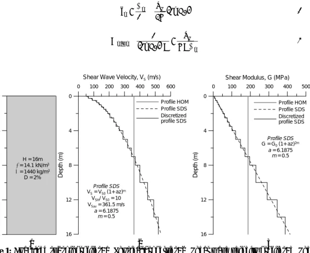
A homogeneous linear visco-elastic layer (denoted as HOM) based on both rigid and elastic bedrock is considered. The examined subsoil profile and its properties are reported in Figure 1a. For this type of subsoil, the theory of the vertical S-wave propagation in the linear visco-elastic media gives a closed form solution of the problem in the frequency domain. Such a system is completely described by means of its amplification function A(f), defined as the modulus of the transfer function, which is the ratio of the Fourier spectrum of amplitude motion at the free surface to the corresponding spectrum of the bedrock motion.

If the properties of the visco-elastic medium (density, ρ or total unit weight of soil, γ; shear wave

velocity, VS; damping ratio, D) and its geometry (layer thickness, H) are known, the amplification

function is univocally defined.

For a soil layer on rigid bedrock, the amplification function (Roesset, 1970) is:

( )

( )

where F is the frequency factor, defined as F = ω H/VS = 2πf H/VS.

For a given linear visco-elastic stratum and a given seismic motion acting at the rigid bedrock, the motion at the free surface can be easily obtained from the amplification function. First, the Fourier spectrum of the input signal is computed. Then, this function is multiplied by the amplification function and finally the motion is given by the inverse Fourier transform of the previous product.

Figure 2 shows its graphical representation in the amplification ratio vs. frequency plane, assuming the adopted soil layer parameters.

The two vertical dashed grey lines remark the first and the second natural frequencies of the system. In the previously listed hypotheses, the n-th natural frequency fn and the maximum amplification ratio

Amax,n of the layer can be computed by means of the following approximated relationships:

(

)

(

)

Figure 1: Examined subsoil profiles: a) Physical properties; b) Shear wave velocity profiles; c) Shear

modulus profiles

Figure 2: Amplification function for homogeneous visco-elastic layer on rigid bedrock.

16 12 8 4 0 Depth (m ) H = 16m γ = 14.1 kN/m3 ρ= 1440 kg/m3 D = 2% 0 100 200 300 400 500 600

Shear Wave Velocity, VS (m/s)

16 12 8 4 0 De pt h (m) Profile HOM Profile SDS Discretized profile SDS Profile SDS VS = VS0 (1+ az)m VSH/ VS0 = 10 V_Sav = 361.5 m/s a = 6.1875 m = 0.5 0 100 200 300 400 500

Shear Modulus, G (MPa)

16 12 8 4 0 De pt h (m ) Profile HOM Profile SDS Discretized profile SDS Profile SDS G = G0 (1+ az)2m a = 6.1875 m = 0.5 0 5 10 15 20 25 Frequency (Hz) 0 10 20 30 40 Am pli fi c atio n R a tio 1st _{Natural Frequency} f₁ = 5.65 Hz 2 nd _{Natural Frequency} f1 = 16.95 Hz

a) b)

c)

Linear elastic layer with stiffness increasing along the depth

A soil stiffness profile cannot be usually represented by a single value of the shear modulus G. In a soil layer, the stiffness increases with the effective mean stress p’, hence with the depth.

Assuming a linear law to describe the evolution of the shear modulus G with the depth z (power exponent m = 1/2):

(

)

(

)

and a constant value of the density ρ, the shear wave velocity profile has the following equation:

(

)

(

)

In the equation (5) VS0 indicates the shear wave velocity VS on the free surface and a is a coefficient

which represents the level of heterogeneity.

Figure 1 plots the stiffness, the shear wave velocity and the damping ratio profiles for the subsoil profile (denoted as SDS, Stress Dependent Stiffness profile). The discretized profiles adopted in the analyses are reported in the same figure.

Nonlinear soil layer

It is well-known that both the shear modulus and the damping ratio depend on the shear strain level. To describe the decay of the shear modulus and the increase of the damping ratio, different curves were proposed in literature for various types of soils (Hardin and Drnevich, 1972; Vucetic and Dobry, 1991). In this study, average values curves for sand and gravel as proposed by Seed and Idriss (1970) were assumed. Figure 3 shows their graphical representations.

The evolution of the initial shear modulus with the depth is the same described for the SDS profile. Different strategies were proposed to account for soil non-linearity using numerical methods. Here, the equivalent linear approach, as proposed by Idriss and Seed (1968) and implemented in the EERA code

(Bardet et al., 2000), the nonlinear hysteretic model, as developed by Iwan (1967) and Mroz (1967) (IM

model) and implemented in the NERA code (Bardet and Tobita, 2001), and the modified nonlinear

hysteretic model (Hashash and Park, 2001) and implemented in the DEEPSOIL code (Hashash et al.,

2008) were used in the dynamic nonlinear analyses.

Figure 3: Shear modulus (continuous line) and damping ratio (dashed line) curves assumed and

calculated from IM model (dash-dot line).

0.0001 0.001 0.01 0.1 1 10 Shear strain, γ (%) 0 0.2 0.4 0.6 0.8 1 G/G ma x 0 10 20 30 40 50 D a m p in g r a ti o, D (%) Shear Modulus Damping ratio Calculated damping ratio

Seismic input motions

In numerical computation, the earthquake loading is often imposed as an acceleration time-history at the base of the model.

To highlight the influence of the input motion on the nonlinear seismic response of a soil layer, two earthquake signals were considered.

The first is the WE component of the accelerometer registration at Tolmezzo Station for the main shock of the earthquake of Friuli (Italy) on May 6th, 1976, denoted as TMZ-270. The data were sampled at 200 Hz for a total number of 7279 registration points. The horizontal peak acceleration, equal to 0.315 g, was reached at the time t=3.935 s. Most of the energy is included into a frequency range between 0.8 and 5 Hz, with a predominant frequency of 1.5 Hz. The Arias intensity is 1.20 m/s and the significant duration (Trifunac and Brady, 1975) is 4.92 s. The time-history of acceleration and the Fourier spectrum of amplitude are reported in Figure 4.

The second is the WE component of the accelerometer registration at Sturno Station for the main shock of the earthquake of Irpinia (Italy) on November 23rd, 1980, denoted as STU-270. The sampling frequency is 400 Hz for a total number of 15737 registration points. The horizontal peak acceleration, equal to 0.321g, was reached at the time t = 5.2375 s. The predominant frequency is 0.44 Hz. The Arias intensity and the significant duration are 1.39 m/s and 15.2 s, respectively. The acceleration time-history and the Fourier spectrum of amplitude are plotted in Figure 5.

Figure 4: TMZ-270 Seismic input signal: a) acceleration time-history; b) Fourier spectrum.

Figure 5: STU-270 Seismic input signal: a) acceleration time-history; b) Fourier spectrum.

0 10 20 30 40 Time (sec) -0.4 -0.2 0 0.2 0.4 Ac cel e rat io n ( g ) 0 5 10 15 20 25 Frequency (Hz) 0 0.05 0.1 0.15 0.2 0.25 F o u rier A m pl itud e (g -sec) 0 10 20 30 40 Time (sec) -0.4 -0.2 0 0.2 0.4 Ac cel e rat io n ( g ) 0 5 10 15 20 25 Frequency (Hz) 0 0.05 0.1 0.15 0.2 0.25 F o u rier A m pl itud e (g -sec)

a)

a)

b)

a)

b)

BRIEF DESCRIPTION OF THE USED NUMERICAL CODES

In the present research, four numerical codes were used to perform the site response analyses for the subsoil profile previously described.

In the following a brief description of each code is reported.

EERA code

EERA (Bardet et al., 2000) stands for Equivalent-linear Earthquake site Response Analysis. It is a

modern implementation of the well-known concepts of the equivalent linear site response analysis that

was first implemented in the SHAKE code (Schnabel et al., 1972). The input and output are fully

integrated with the spreadsheet program MS-Excel.

This code permits to perform frequency domain analyses for linear and equivalent linear stratified subsoils.

The bedrock can be modelled as rigid, if the option “inside” is selected in the Profile spreadsheet of

the program, or as elastic, by assigning its properties to the last layer and selecting the option “outcrop”

in the Profile spreadsheet.

In order to transform the signal from the outcropping rock to the bedrock, placed at the bottom of the soil layer, EERA applies a suitable transfer function to the input signal.

NERA code

NERA (Bardet and Tobita, 2001) stands for Nonlinear Earthquake site Response Analysis. It allows solving the 1-D vertical shear wave propagation in a nonlinear hysteretic medium in the time domain. The constitutive model implemented in NERA is that proposed by Iwan (1967) and Mroz (1967), IM model, which simulates nonlinear stress-strain curves using a series of n mechanical elements, having different

stiffness ki and sliding resistance Ri. The IM model assumes that the hysteretic stress-strain loop follows the Masing rules. For this reason, the damping ratio curves directly derive from the G/Gmax(γ) curves and,

then, they cannot be defined independently as in the case of the equivalent linear model. Therefore, the damping ratio curves that derive from the IM model are shown and compared with the assumed curves in the previously presented Figure 3.

The central difference method is used to perform the 1-D time domain analyses by adopting a finite difference formulation.

PLAXIS code

PLAXIS (Brinkgreve, 2002) is a commercial finite element code that allows performing stress-strain analyses for various types of geotechnical systems.

An earthquake analysis can be performed by imposing an acceleration time-history at the base of the FE model and solving the equations of motion in the time domain by adopting a Newmark type implicit time integration scheme.

DEEPSOIL code

DEEPSOIL (Hashash et al., 2008) is a program for the one-dimensional site response that performs

The code has a graphical user-interface that allows selecting the modes/frequencies of the viscous damping formulation and the nonlinear soil parameters. The modified hyperbolic model (Hashash and Park, 2001) implemented in the code permits to account for stress- and strain- dependency of the soil behaviour by means of an appropriate definition of the model parameters that can be simply done by using a fitting curve procedure fully automated in the program.

The 1-D time domain analyses are performed by using a Newmark (1959) method to solve the dynamic equations of the motion on a lumped mass scheme. For saturated subsoils, the program allows also conducting wave propagation analysis with pore water pressure generation and dissipation.

The used version of the code is the DEEPSOIL v.3.5 Beta.

NUMERICAL RESULTS AND DISCUSSIONS

For the assumed subsoil profiles and for the seismic input motions presented in the previous sections, different analyses were conducted to highlight the influence of some numerical parameters. Here, the results obtained from linear analyses for the homogeneous profile (HOM) and for the stress-dependent soil stiffness profile (SDS) are shown. Then, the use of the equivalent linear approach for time domain analyses with the PLAXIS code is presented and the results are compared with those obtained from the frequency domain analyses performed with the EERA code. Finally, the comparisons between the ground motion estimations provided by the different numerical codes are discussed.

Sources of energy dissipation in the time domain analyses

In a dynamic finite element analysis different sources of energy dissipation exist: material damping, which includes viscous and hysteretic soil damping, numerical damping, arising from the adopted time integration scheme, and energy dissipation at the boundaries. Visone et al. (2010) extensively discussed

this topic. In this subsection the main issues are summarized.

For a linear elastic material, the area bounded by stress-strain loops is zero and then, there is not hysteretic damping.

However, laboratory tests (e.g. Hardin and Drnevich, 1972; Tatsuoka et al. 1978) have clearly shown

the presence of damping at very small strains, too. Numerically, this problem can be overcome by introducing viscous dashpots embedded within linear elastic elements. In most dynamic FE codes, such

viscous damping is simulated according to the well-known Rayleigh formulation. The damping matrix C

is assumed to be proportional to the mass matrix M and the stiffness matrix K by means of two

coefficients, αR and βR such as:

K M

C=α_R +β_R (6)

Different criteria exist to evaluate the Rayleigh coefficients (see for instance Hashash and Park, 2002; Lanzo et al., 2004; Park and Hashash, 2004). The dynamic response of a system is significantly affected

by the choice of these parameters.

In the PLAXIS code, the Rayleigh damping formulation is implemented and the values of αR and βR

can be estimated with the system of equations:

* ni 2 ni R R+β ω =2ω D α (7)

in which D* is the assumed value for the damping ratio and ωni are two circular natural frequencies of the

In the numerical implementation of dynamic problems, the formulation of the time integration algorithm is an important factor for stability and accuracy of the calculation process. Explicit and implicit integration are two commonly used time integration schemes. In the FE code Plaxis 2D v.8.2 (Brinkgreve, 2002), the Newmark type implicit time integration scheme is implemented. Within this method, the displacement and the velocity of any point at time t+Δt are expressed respectively as:

2 t t N t N t t t t _{u u t} 2 1 t u u u Δ      α +       α − + Δ + = +Δ Δ + _{   (8)}

(

)

[

]

The coefficients αN and βN control the accuracy of the numerical time integration. They can be chosen

by following the Newmark HHT modification scheme (Hilber et al., 1977) as:

(

)

where the value of γ belongs to the range [0, 1/3]. By assuming γ>0 the efficiency of the calculation is improved, but a numerical source of damping is introduced into the model.

The choice of boundary conditions influences the amount of energy dissipation due to the wave propagation in the ground. The position of the boundary and the kind of mechanical constraints should reproduce, at best, the energy transmission outwards the computation domain. Viscous adsorbent boundaries based on the method described by Lysmer and Kuhlemeyer (1969) are a rather widespread procedure. In this case, normal and tangential stress components adsorbed at the boundary location are:

1 n c V uP n σ = − ρ  (12) 2 S t c V u τ= − ρ  (13)

where ρ is the density of the material, VP and VS are the compression and shear wave velocities, unandut are the normal and tangential components of the velocity, c1 and c2 are relaxation coefficients. Some

suggestions exist in literature for the choice of these parameters.

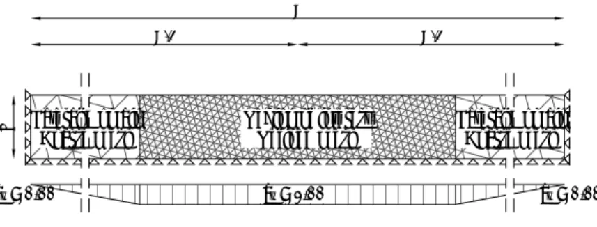
The numerical model sketched in Figure 6 of a simple soil column with vertical fixities on the lateral boundaries and total fixities at the bottom was used to calibrate the damping parameters in the time domain analyses. When a more complex constitutive law, such as elastic-plastic models, or geometry configuration should be analyzed, the soil column is not suitable for the calculation. In these cases, a FE configuration for the dynamic analyses could be that sketched in Figure 7. The region of interest is constituted only by the central domain. The two lateral domains, characterized by a coarse mesh, to reduce the computational costs, and a tapered input motion, have the aim to minimize the spurious effects of reflection on the boundaries. In spite of higher calculation time respect to other silent boundary conditions (Ross, 2004), such a solution allows minimizing the boundaries effects.

Figure 6: Sketch of the used FE model for the calibration of the damping parameters.

Linear analyses for the HOM profile

In order to show the influence of the different sources of the energy dissipation on the seismic response of the FE models and to highlight the choices for a good numerical modelling procedure, linear frequency and time domain analyses were performed and compared for the elementary case of the homogeneous elastic layer laying on both rigid and elastic bedrock.

Figure 7: Sketch of the FE model with the adopted silent lateral boundaries.

In the following, the results of the calculations are presented.

Rigid bedrock

As above mentioned, for the HOM profile lying on a rigid bedrock, the amplification function assumes an analytical expression, reported in the Equation (1).

The results of the linear frequency and time domain analyses performed by EERA and PLAXIS codes, respectively, are shown in Figure 8, in terms of amplification function (Figure 8a) and maximum acceleration profiles (Figure 8b,c).

The dynamic finite element computations were conducted by using the soil column model (Figure 6) and adopting a constant average acceleration scheme (γ = 0). The calculation time-step dt is taken equal to 0.5ms to respect the accuracy condition suggested by Brinkgreve (2002). The Rayleigh damping parameters were calculated according to the system (7) taking the first (f1 = 5.65 Hz) and the second (f2 =

16.95 Hz) natural frequencies of the layer. As expected, the curves given by the two types of analyses are the same.

The standard setting of the PLAXIS code for time integration is a damped Newmark scheme with γ =

0.1, that corresponds to αN = 0.3025 and βN = 0.6. In order to quantify the numerical dissipation due to the

time integration scheme, further analyses were conducted for other homogeneous layers with various

ax(t) K0γz K0γH K0γH H = 16m B K0γz ax = 1.00 ax = 0.00 ax = 0.00 H B/2 B/2 B Region of interest

Refined Mesh Lateral DomainCoarse Mesh

Lateral Domain Coarse Mesh

values of thickness, damping ratio and shear wave velocity. The results have suggested the following relationship for the formulation of the modal damping of the system:

(

)

Equation (14) represents the extension of the Rayleigh damping formulation to take into account the numerical dissipation when a damped Newmark integration scheme is used.

Figure 8: Comparisons between numerical and reference solutions: a) amplification functions; b)

maximum acceleration profiles for TMZ-270 input motion; c) maximum acceleration profiles for STU-270 input motion.

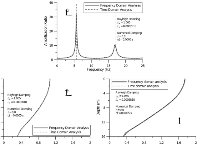
Figure 9 shows the validity of the adopted material and numerical damping formulation for the HOM profile laying on rigid bedrock. As a matter of fact, the results of the time domain analysis coincides with those of the frequency domain analysis.

Elastic bedrock

If the bedrock is rigid, its motion is not affected by the presence of the overlying soil. It acts as a fixed end boundary. Any downward-travelling waves in the soil is completely reflected back toward the ground surface by the rigid layer, thereby trapping all of the elastic wave energy within the soil layer.

0 5 10 15 20 25 Frequency (Hz) 0 10 20 30 40 Ampl ifi c a tio n Ra ti o

Frequency Domain Analyses Time Domain Analysis

Rayleigh Damping αR = 1.065 βR = 0.0002818 Numerical Damping γ = 0.0 dt = 0.0005 s 0 0.4 0.8 1.2 1.6 2 Maximum Acceleration (g) 16 12 8 4 0 De pt h ( m )

Frequency Domain Analysis Time Domain Analysis Rayleigh Damping αR = 1.065 βR = 0.0002818 Numerical Damping γ = 0.0 dt = 0.0005 s 0 0.4 0.8 1.2 1.6 2 Maximum acceleration (g) 16 12 8 4 0 De pt h ( m )

Frequency domain analysis Time domain analysis Rayleigh Damping αR = 1.065 βR = 0.0002818 Numerical Damping γ = 0.0 dt = 0.0005 s

a)

b)

c)

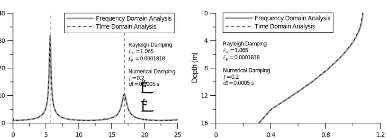
Figure 9: Comparisons between frequency and time domain analyses using TMZ-270 seismic motion for

a combination of numerical and Rayleigh damping parameters according to Equation (14): a) amplification functions; b) maximum acceleration profiles.

In a time domain analysis, the rigid bedrock is simply modeled imposing an acceleration (or velocity or displacement) time-history at the base of the numerical model, as shown in the previous subsection.

If the rock is elastic, however, downward-travelling stress waves that reach the soil-rock boundary are reflected only partially; part of their energy is transmitted through the boundary to continue travelling downward through the rock. If the rock extends to great depth, the elastic energy of these waves is effectively removed from the soil layer. This is a form of radiation damping and it causes the free surface motion amplitudes to be smaller than those for the case of rigid bedrock.

For a uniform visco-elastic soil layer based on an elastic rock, the amplification function cannot be

expressed in a very compact form. The expression of the maximum amplification ratio Amax,n in

correspondence of the natural frequencies of the layer is (Roesset, 1970):

(

)

in which I = ρRVSR/ρSVS indicates the impedance ratio between the seismic impedances of the rock ρRVSR

and of the soil ρSVS.

In a time domain analysis, the presence of an elastic bedrock can be modelled by imposing a force time history rather than a base motion at the bottom of the soil layer. The continuity of the stresses along the rock-soil boundary requires that the shear stress in the rock side is equal to the shear stress in the soil side. For this reason, the motion of an elastic bedrock is usually specified by adopting a shear stress time history τ(t). It can be simply obtained by the motion expected at the outcropping rock in terms of velocity time-history u

( )

( )

( )

τ (16)

where ρR and VSR are the mass density and the shear wave velocity of the elastic bedrock.

Another way to specify the motion of an elastic bedrock at the bottom of a FE model is to run a frequency domain analysis by applying the seismic signal at the outcropping rock and then computing the time-history of acceleration at the interface between the soil layer and the rock (called “inside” in the EERA code). Such time history accounts for the shear stress transmission between the bedrock and the layer and can be directly applied to the lower boundary of the FE mesh. This approach is used here.

0 5 10 15 20 25 Frequency (Hz) 0 10 20 30 40 Amp lif ic at ion Ra ti o

Frequency Domain Analysis Time Domain Analysis

Rayleigh Damping αR = 1.065 βR = 0.0001818 Numerical Damping γ = 0.2 dt = 0.0005 s 0 0.4 0.8 1.2 Maximum Acceleration (g) 16 12 8 4 0 De pth (m)

Frequency Domain Analysis Time Domain Analysis Rayleigh Damping αR = 1.065 βR = 0.0001818 Numerical Damping γ = 0.2 dt = 0.0005 s

a)

b)

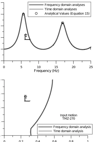
Figure 10 shows the results evaluated by the EERA (frequency domain) and PLAXIS (time domain) codes for the HOM layer lying on an elastic bedrock characterized by the properties given in Table 1.

Table 1: Elastic bedrock parameters used in the analyses

The linear time domain analyses was performed by using the constant average acceleration scheme (γ

= 0) and adopting the same abovementioned values of the Rayleigh damping parameters (αR=1.065;

βR=2.818·10-4). The input motions for these types of analysis are constituted by the “inside” bedrock

acceleration time histories calculated by the EERA code, both for TMZ-270 and STU-270 seismic signals. As expected in the linear elasticity field, the amplification functions, defined as the ratio of the ground surface and outcropping rock motions, are the same for the two input signals. The analytical values of the maximum amplification ratio computed by means of the Equation (15) are reported and compared with the numerical values in the same figure. Little differences between numerical and analytical solutions can be noted, both for the 1st _{and the 2}nd _{vibration mode. The natural frequencies (f}

1 =

5.62 Hz; f2 = 16.92 Hz) of the layer are very similar to the corresponding for the case of rigid bedrock (f1

= 5.65 Hz; f2 = 16.95 Hz). It can also be noted the smaller amplification of the motion respect to the cases

of rigid bedrock (see Figure 8).

0 5 10 15 20 25 Frequency (Hz) 0 1 2 3 4 5 Ampl if ic at io n ra ti o

Frequency domain analyses Time domain analyses Analytical Values (Equation 15)

0 0.2 0.4 0.6 0.8 1 Maximum acceleration (g) 16 12 8 4 0 Depth (m)

Frequency domain analysis Time domain analysis

Input motion TMZ-270

b)

a)

Figure 10: Comparisons between frequency and time domain linear analyses for HOM profile lying on

elastic bedrock: a) amplification functions; b) maximum acceleration profiles for TMZ-270 input motion; c) maximum acceleration profiles for STU-270 input motion.

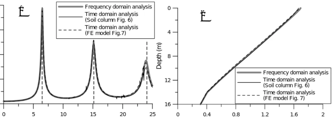
Linear analyses for the SDS profile

Linear analyses have been conducted in the frequency domain for TMZ-270 using the EERA code and the results were used as reference solution for the PLAXIS analyses. The latter were performed both on the elastic column (Figure 6) and on the FE mesh of a layer in Figure 7. The values of the Rayleigh damping coefficients (αR = 1.224; βR = 2.441x10-4) were arbitrarily evaluated by choosing as targets the

1st _{natural frequency of the layer, f}

1, and the average value (f2 + f3)/2, where f2 and f3 are the 2nd and the

3rd _{natural frequency of the subsoil. The numerical damping was assumed equal to zero. Figure 11 shows}

the results obtained for the soil column and for the layer. Only around the third natural frequency of the layer, some differences can be noted on the amplification functions. Instead, the maximum acceleration profiles are in very good agreement. This shows the effectiveness of the adopted lateral boundary conditions.

Figure 11: Comparisons between soil column (Figure 6) and stratum with the adopted lateral boundary

conditions (Figure 7) for the SDS profile (TMZ-270 seismic input motion): a) amplification functions; b) maximum acceleration profiles.

0 0.2 0.4 0.6 0.8 1 Maximum acceleration (g) 16 12 8 4 0 Depth (m)

Frequency domain analysis Time domain analysis

Input motion STU-270 0 5 10 15 20 25 Frequency (Hz) 0 10 20 30 40 Amplif ication ratio

Frequency domain analysis Time domain analysis (Soil column Fig. 6) Time domain analysis (FE model Fig.7)

0 0.4 0.8 1.2 1.6 2 Maximum acceleration (g) 16 12 8 4 0 De pt h ( m )

Frequency domain analysis Time domain analysis (Soil column Fig. 6) Time domain analysis (FE model Fig. 7)

c)

b)

a)

Equivalent-Linear analyses for SDS profile

To model the nonlinearity of the soil stress-strain response under cyclic loadings, the first and the most common method is the equivalent linear approach (Idriss and Seed, 1968) implemented in EERA.

The PLAXIS code would not permit to carry out equivalent linear analyses. To perform such kind of calculation, the domain needs to be divided into sublayers and a different material shall be specified for each sublayer. Therefore, a possible solution is to run preliminarily an equivalent linear analysis by means of the EERA code, which performs an automatic iterative procedure. The final profile of G(z) and D(z) calculated by EERA can be then used to define the material parameters in PLAXIS (Bilotta et al., 2007; Visone et al., 2010).

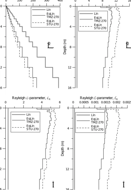
In Figure 12 the initial shear modulus and the damping ratio profiles are plotted together with those derived from the EERA analysis that constituted the input profiles for the Plaxis code. Also, the adopted values for the Rayleigh damping parameters are indicated. The procedure was adopted for both TMZ-270 and STU-270 input signals.

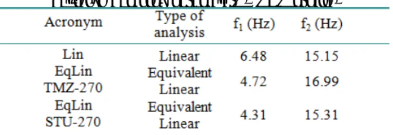
The results obtained by the numerical analyses using the equivalent linear approach in the frequency and in the time domains are plotted in Figure 13. The used time integration scheme is the constant average acceleration (γ = 0) and the Rayleigh parameters of each sublayer are evaluated according to the Equation (14). The 1st _{and the 3}rd _{natural frequencies of the subsoil, reported in Table 2, are assumed as}

target frequencies. Calibrating the numerical parameters for the time domain analyses on the basis of the results of the frequency domain, the two types of equivalent linear approaches give similar ground motion estimations, especially in terms of maximum acceleration profiles.

Table 2: Assumed target frequencies, f1 and f2, for the evaluation of

Rayleigh damping parameters - SDS profile.

The peaks of the amplification functions evaluated with the FE code are close to the corresponding values of EERA, especially near to the target frequencies. These results showed that, as previously specified, the values of the soil parameters defined for each sublayer are consistent with the level of strain induced by the seismic motion.

Nonlinear analyses for SDS profile

It is well known that equivalent linear approach is computationally convenient and provides reasonable results, especially for the seismic ground response, but it remains an approximation to the actual non-linear processes (Kramer, 1996). An alternative approach is to analyze the actual nonlinear response of a soil deposit using direct numerical integration in the time domain.

Figure 12: Profiles of soil parameters adopted in the equivalent linear analyses: a) Shear moduli; b)

Damping ratios; c) Rayleigh α-parameters; d) Rayleigh β-parameters

The NERA and the DEEPSOIL codes allow solving the 1-D wave propagation problems in non-linear media. The analyses are performed in the time domain and the implemented constitutive models are the previously presented IM model (see § 4.2), for NERA, and the modified hyperbolic model (Hashash and Park, 2001), for DEEPSOIL. These programs were used to analyze the problem of the vertical propagation of S-waves into the nonlinear SDS profile lying on both rigid and elastic bedrock and to compare the results with those obtained adopting the equivalent linear approach.

Figure 14 shows the maximum acceleration profiles and the response spectra computed by means of the EERA, the NERA and the DEEPSOIL codes adopting the shear modulus and the damping ratio curves plotted in Figure 3 for the case of rigid bedrock. Both of TMZ-270 and STU-270 input motions were used in the calculations. In the NERA code, the boundary condition of the rigid bedrock at the bottom of the soil layer was simulated by using a very high value of rock seismic impedance. The model parameters for the DEEPSOIL analyses were evaluated by fitting the soil data with the procedure implemented in the program. It can be noted the smaller values of the maximum accelerations at surface

0 100 200 300 400

Shear Modulus, G (MPa)

16 12 8 4 0 De pth (m) Lin EqLin TMZ-270 EqLin STU-270 0 4 8 12 16 Damping ratio, D (%) 16 12 8 4 0 De pt h ( m ) Lin EqLin TMZ-270 EqLin STU-270 0 2 4 6 Rayleigh α-parameter, αR 16 12 8 4 0 D ept h (m ) Lin EqLin TMZ-270 EqLin STU-270 0 0.0005 0.001 0.0015 0.002 0.0025 Rayleigh β-parameter, βR 16 12 8 4 0 De pth (m) Lin EqLin TMZ-270 EqLin STU-270

a) b)

c) d)

given by the two types of nonlinear analyses respect to the corresponding values of the equivalent linear approach.

Figure 13: Comparisons between equivalent linear frequency domain (EERA) and time domain

(PLAXIS) analyses for SDS profile: amplification functions (a) and maximum acceleration profiles (b) for TMZ-270; amplification functions (c) and maximum acceleration profiles (d) for STU-270.

In particular, the lower values of the maximum acceleration are those predicted by the NERA code that, instead, conducts to the higher values for the deeper sublayers, near to the bedrock.

It can also be seen the higher values of the spectral acceleration into the range 0.1÷1s, that corresponds to the range of frequencies 1÷10Hz, where the frequency contents of the input signals are concentrated. 0 5 10 15 20 25 Frequency (Hz) 0 2 4 6 8 10 A m pl if ic at ion r a ti o

Frequency domain analysis Time domain analysis

0 5 10 15 20 25 Frequency (Hz) 0 2 4 6 8 10 Amp lif ica tio n ra tio

Frequency domain analysis Time domain analysis

0 0.4 0.8 1.2 Maximum acceleration (g) 16 12 8 4 0 De pt h (m)

Frequency domain analysis Time domain analysis

0 0.4 0.8 1.2 Maximum acceleration (g) 16 12 8 4 0 De pt h (m)

Frequency domain analysis Time domain analysis

0 0.4 0.8 1.2 Maximum acceleration (g) 16 12 8 4 0 De pth (m) Equivalent linear FD analysis - EERA Nonlinear TD analysis NERA Nonlinear analysis TD DEEPSOIL Rigid bedrock Input motion TMZ-270 0 0.4 0.8 1.2 Maximum acceleration (g) 16 12 8 4 0 De pt h ( m ) Equivalent linear FD analysis - EERA Nonlinear TD analysis NERA Nonlinear analysis TD DEEPSOIL Rigid bedrock Input motion STU-270

b)

a)

d)

c)

For the periods lower than 0.1s, hence, for high frequencies, the equivalent linear approach provides smaller spectral acceleration values.

The same qualitative results were obtained for the case of the elastic bedrock, as can be deduced from the Figure 15.

Figure 14: Seismic site response computed by the codes EERA (equivalent linear analyses), NERA and

DEEPSOIL(nonlinear analyses) for the SDS profile lying on rigid bedrock: a) TMZ-270 input motion; b) STU-270 input motion.

Figure 15: Seismic site response computed by codes EERA (equivalent linear analyses), NERA and

DEEPSOIL(nonlinear analyses) for the SDS profile lying on elastic bedrock: a) TMZ-270 input motion; b) STU-270 input motion

0.01 0.1 1 10 Period (sec) 0 2 4 6 Sp ec tr al ac cel e ration (g ) Equivalent linear FD analysis EERA Nonlinear TD analysis NERA Nonlinear TD analysis DEEPSOIL Rigid bedrock Input motion TMZ-270 0.01 0.1 1 10 Period (sec) 0 2 4 6 Spe c tr al ac cel e ration (g) Equivalent linear FD analysis EERA Nonlinear TD analysis NERA Nonlinear TD analysis DEEPSOIL Rigid bedrock Input motion STU-270 0 0.4 0.8 1.2 Maximum acceleration (g) 16 12 8 4 0 De pth (m) Equivalent linear FD analysis - EERA Nonlinear TD analysis NERA Nonlinear analysis TD DEEPSOIL Elastic bedrock Input motion TMZ-270 0 0.4 0.8 1.2 Maximum acceleration (g) 16 12 8 4 0 De pth (m) Equivalent linear FD analysis - EERA Nonlinear TD analysis NERA Nonlinear analysis TD DEEPSOIL Elastic bedrock Input motion STU-270 0.01 0.1 1 10 Period (sec) 0 2 4 6 Sp ec tr al a c c e le ration (g ) Equivalent linear FD analysis EERA Nonlinear TD analysis NERA Nonlinear TD analysis DEEPSOIL Elastic bedrock Input motion TMZ-270 0.01 0.1 1 10 Period (sec) 0 2 4 6 Sp ec tr al a c c e le ration (g ) Equivalent linear FD analysis EERA Nonlinear TD analysis NERA Nonlinear TD analysis DEEPSOIL Elastic bedrock Input motion STU-270

a) b)

a) b)

CONCLUSIONS

One-dimensional nonlinear ground response analyses provide a more accurate characterization of the true nonlinear soil behaviour than equivalent-linear procedures, but the application of nonlinear codes in practice has been limited, which results in part from poorly documented and unclear parameter selection and code usage protocols.

In this paper, the linear frequency domain solutions were used to establish guidelines for the evaluation of the sources of energy dissipation related to dynamic FE analyses. The calculations performed by using PLAXIS code have shown the effectiveness of the adopted numerical modelling choices, both for the estimation of the Rayleigh damping parameters, taking into account the numerical dissipation for a modified Newmark time integration scheme, and for the lateral boundary conditions, to minimize the spurious effects due to the waves reflection.

The obtained results encourage to use of such suggestions every time seismic finite element analyses should be performed on various types of geotechnical system (e.g. retaining walls, pile foundations, tunnels, etc.).

Also, the specification of the base shaking in the numerical analyses was discussed. When the input motion is recorded at the ground surface (e.g., at a rock site) the full outcropping rock motion should be applied to an elastic base having a stiffness appropriate for the underlying rock (Kwok et al., 2007). In some FE codes, as in PLAXIS, the signal “filtering” to transform the input motion from the outcropping to the inside rock is not implemented. Then, it is proved here that, to simulate an elastic bedrock under a FE model, the input signal can be simply transformed from outcrop to inside by using other codes (e.g., EERA code) and applying the filtered signal at the bottom of the model.

Finally, the soil nonlinear behaviour was considered. First, the equivalent linear approach implemented in the EERA code was used to calibrate the numerical parameters of the FE models developed in PLAXIS. Then, nonlinear analyses adopting NERA and DEEPSOIL codes were performed and the results are compared with those obtained by the equivalent linear approach. For the examined profile, equivalent linear method gives higher values of the maximum acceleration at surface than the nonlinear analyses. This can be attributed to the larger amplification of the motion components characterized by frequencies close to the predominant frequencies of the adopted seismic motions.

REFERENCES

1. Bardet J.P., Ichii K. and Lin C.H. (2000) “EERA: a computer program for Equivalent-linear

Earthquake site Response Analyses of layered soil deposits”, University of Southern California, Los Angeles.

2. Bardet J.P., Tobita T. (2001) “NERA: a computer program for Nonlinear Earthquake site

Response Analyses of layered soil deposits”, University of Southern California, Los Angeles.

3. Bilotta E., Lanzano G., Russo G., Santucci de Magistris F., Silvestri F. (2007) “Methods for the

seismic analysis of transverse section of circular tunnels in soft ground”. Workshop of ERTC12 - Evaluation Committee for the Application of EC8 Special Session XIV ECSMGE, Madrid, Patron Ed., Bologna.

4. Brinkgreve R.B.J. (2002) “Plaxis 2D version8” A.A. Balkema Publisher, Lisse.

5. EPRI, Electric Power Research Institute (1991) “Soil response to earthquake ground motion”,

6. Hardin B.O. and Drnevich V.P. (1972) “Shear modulus and damping in sands, I. Measurement and parameter effects”, Technical Report No. UKY 26-70-CE2, University of Kentucky, College of Engineering, Soil Mechanics Series No.1, Lexington, Ky.

7. Hashash Y.M.A., and Park D. (2001) “Non-linear one-dimensional seismic ground motion

propagation in the Mississipi embayment”, Elsevier, Engineering Geology, 62, pp. 185-206

8. Hashash Y.M.A., and Park D. (2002) “Viscous damping formulation and high frequency motion

propagation in nonlinear site response analysis”, Elsevier, Soil Dynamics and Earthquake Engineering, 22, pp. 611-624

9. Hashash Y.M.A., Groholski D.R., Philips C.A., and Park D. (2008) “DEEPSOIL v3.5beta: User

Manual and Tutorial”, 84 pp.

10. Idriss I.M., and Seed H.B. (1968) “Seismic response of horizontal soil layers”, ASCE, Journal of

the Soil Mechanics and Foundation Division, 94(4), pp.1003-1031

11. Iwan W.D. (1967) “On a class of models for the yielding behaviour of continuous and composite

systems”, ASME, Journal of Applied Mechanics, 34, pp.612-617

12. Kramer, S.L. (1996) Geotechnical Earthquake Engineering, Prentice Hall, Inc., Upper Saddle

River, New Jersey, 653 pp.

13. Kuhlemeyer R.L and Lysmer J. (1973) “Finite Element Method Accuracy for Wave Propagation

Problems”, Journal of the Soil Mechanics and Foundation Division, 99(5), 421-427.

14. Kwok A.O.L., Stewart J.P., Hashash Y.M.A., Matasovis N., Pyke R., Wang Z., Yang Z. (2007)

“Use of exact solutions of wave propagation problems to guide implementation of nonlinear seismic ground response analysis procedures”, ASCE, Journal of Geotechnical and Geoenvironmental Engineering, 133 (11), pp. 1385-1398.

15. Lanzo G., Pagliaroli A. and D’Elia B. (2004) “L’influenza della modellazione di Rayleigh dello

smorzamento viscoso nelle analisi di risposta sismica locale”, ANIDIS, XI Congresso Nazionale “L’Ingegneria Sismica in Italia”, Genova 25-29 Gennaio 2004 (in Italian).

16. Lanzo G. (2005) “Risposta sismica locale”, Aspetti geotecnici della progettazione in zone

sismiche, Linee Guida AGI (in Italian).

17. Hilber H.M., Hughes T.J.R., Taylor R.L. (1977) “Improved numerical dissipation for time

integration algorithms in structural dynamics”, Earthquake Engng Struct. Dynamics, 5, pp. 283-292.

18. Lysmer J. and Kuhlemeyer R.L. (1969) “Finite Dynamic Model for Infinite Media”, ASCE,

Journal of Engineering and Mechanical Division, 859-877.

19. Lysmer J. (1978) “Analytical procedures in soil dynamics”, Report no. UCB EERC-78/29,

University of California, Berkeley

20. Mroz Z. (1967) “On the description of anisotropic work hardening”, Journal of Mechanics and

Physics of Solids, 15, pp. 163-175

21. Newmark N.M. (1959) “A method of computation for structural dynamics” Journal of Engng

Mech Div., 85, pp.67–94.

22. Park D. and Hashash Y.M.A. (2004) “Soil Damping Formulation in Nonlinear Time Domain Site

Response Analysis”, Journal of Earthquake Engineering, 8(2), 249-274.

23. PHRI (1997) Handbook on liquefaction remediation of reclaimed land, Port and Harbour

24. PIANC (2001) “Seismic Design Guidelines for Port Structures”, Working Group n.34 of the Maritime Navigation Commis-sion, International Navigation Association, Balkema, Lisse, 474 pp.

25. Roesset, J.M. (1970). “Fundamentals of Soil Amplification”, in Seismic Design for Nuclear

Power Plants, ed. R.J. Hansen, The MIT Press, Cambridge, MA, pp. 183-244.

26. Roesset J.M. (1977) “Soil Amplification of Earthquakes”, in Numerical Methods in Geotechnical

Engineering, Ed. Desai C.S., Christian J.T. - McGraw-Hill, pp. 639-682.

27. Ross M., (2004) “Modeling Methods for Silent Boundaries in Infinite Media”, ASEN 5519-006:

Fluid-Structure Interaction, University of Colorado at Boulder.

28. Schnabel, P. B., Lysmer, J., and Seed, H. B. (1972) “SHAKE: a computer program for earthquake

response analysis of horizontally layered sites”, Report n° EERC72-12, University of California at Berkeley.

29. Seed H.B., and Idriss I.M. (1970) “Soil moduli and damping factors for dynamic response

analyses”, Report ERC 70-10, Earthquake Engineering Research Center, University of California, Berkeley

30. Tatsuoka F., Iwasaki T., Takagi Y. (1978) “Hysteretic damping of sands and its relation to shear

modulus”, Soils and Foundations, 18(2), 25-40.

31. Trifunac M.D. and Brady A.G. (1975) “A study of the duration of strong earthquake ground

motion”, Bulletin of the Seismological Society of America, 65, 581-626.

32. Tsai N.C. (1969) “Influence of local geology on earthquake ground motions”, PhD Thesis,

California, Institute of Technology, Pasadena.

33. Visone C., Bilotta E., Santucci de Magistris F. (2010) “One-dimensional round response as a

preliminary tool for dynamic analyses in geotechnical earthquake engineering”, Journal of Earthquake Engineering, 14 (1), in print.

34. Vucetic M., and Dobry R. (1991) “Effects of the soil plasticity on cyclic response”, ASCE,

Journal of Geotechnical Engineering Division, 117, 1