Topological Signal Processing over
Simplicial Complexes
Sergio Barbarossa,
Fellow, IEEE
, Stefania Sardellitti,
Member, IEEE
Abstract—The goal of this paper is to establish the fundamental tools to analyze signals defined over a topological space, i.e. a set of points along with a set of neighborhood relations. This setup does not require the definition of a metric and then it is especially useful to deal with signals defined over non-metric spaces. We focus on signals defined over simplicial complexes. Graph Signal Processing (GSP) represents a special case of Topological Signal Processing (TSP), referring to the situation where the signals are associated only with the vertices of a graph. Even though the theory can be applied to signals of any order, we focus on signals defined over the edges of a graph and show how building a simplicial complex of order two, i.e. including triangles, yields benefits in the analysis of edge signals. After reviewing the basic principles of algebraic topology, we derive a sampling theory for signals of any order and emphasize the interplay between signals of different order. Then we propose a method to infer the topology of a simplicial complex from data. We conclude with applications to traffic analysis over wireless networks and to the processing of discrete vector fields to illustrate the benefits of the proposed methodologies.
Index Terms—Algebraic topology, graph signal processing, topology inference.
I. INTRODUCTION
Historically, signal processing has been developed for sig-nals defined over a metric space, typically time or space. More recently, there has been a surge of interest to deal with signals that are not necessarily defined over a metric space. Examples of particular interest are biological networks, social networks, etc. The field of graph signal processing (GSP) has recently emerged as a framework to analyze signals defined over the vertices of a graph [2], [3]. A graph G(V,E) is a simple example of topological space, composed of a set of elements (vertices) V and a set of edges E representing pairwise relations. However, notwithstanding their enormous success, graph-based representations are not always able to capture all the information present in interconnected systems in which the complex interactions among the system constitutive elements cannot be reduced to pairwise interactions, but require a multiwaydescription, as suggested in [4]–[9].
To establish a general framework to deal with complex interacting systems, it is useful to start from a topological space, i.e. a set of elements V, along with an ensemble of multiway relations, represented by a setScontaining subsets
The authors are with the Department of Information Engineering, Electronics, and Telecommunications, Sapienza University of Rome, Via Eudossiana 18, 00184, Rome, Italy. E-mails: {sergio.barbarossa; stefa-nia.sardellitti}@uniroma1.it. This work has been supported by H2020 EU/Taiwan Project 5G CONNI, Nr. AMD-861459-3 and by MIUR, under the PRIN Liquid-Edge contract. Some preliminary results of this work were presented at the 2018 IEEE Workshop in Data Science [1].
of various cardinality, of the elements of V. The structure
H(V,S) is known as ahypergraph. In particular, a class of hypergraphs that is particularly appealing for its rich algebraic structure is given by simplicial complexes, whose defining feature is the inclusion property stating that if a setAbelongs toS, then all subsets ofAalso belong toS[10]. Restricting the attention to simplicial complexes is a limitation with re-spect to a hypergraph model. Nevertheless, simplicial complex models include many cases of interest and, most important, their rich algebraic structure makes possible to derive tools that are very useful for analyzing signals over the complex. Learning simplicial complexes representing the complex inter-actions among sets of elements has been already proposed in brain network analysis [6], neuronal morphologies [11], co-authorship networks [12], collaboration networks [13], [14], tumor progression analysis [15]. More generally, the use of algebraic topology tools for the extraction of information from data is not new: The framework known as Topological Data Analysis(TDA), see e.g. [16], has exactly this goal. Interesting applications of algebraic topology tools have been proposed to control systems [17], statistical ranking from incomplete data [18], [19], distributed coverage control of sensor networks [20]–[22], wheeze detection [23]. One of the fundamental tools of TDA is the analysis of persistent homologies extracted from data [24], [25]. Topological methods to analyze signals and images are also the subjects of the two books [26] and [27].
The goal of our paper is to establish a fundamental frame-work to analyze signals defined over a simplicial complex. Our approach is complementary to TDA: Rather than focusing, like TDA, on the properties of the simplicial complex extracted from data, we focus on the properties of signals defined over a simplicial complex. Our approach includes GSP as a particular case: While GSP focuses on the analysis of signals defined over the vertices of a graph, topological signal processing (TSP) considers signals defined over simplices of various order, i.e. signals defined over nodes, edges, triangles, etc. Relevant examples of edge signals are flow signals, like blood flow between different areas of the brain [28], data traffic over communication links [29], regulatory signals in gene regulatory networks [30], where it was shown that a dysregulation of these regulatory signals is one of the causes of cancer [30]. Examples of signals defined over triplets are co-authorship networks, where a (filled) triangle indicates the presence of papers co-authored by the authors associated to its three vertices [12] and the associated signal value counts the number of such publications. Further examples of even higher order structures are analyzed in [8], with the goal of predicting higher-order links. There are previous works dealing with the
analysis of edge signals, like [31]–[34]. More specifically, in [31] the authors introduced a class of filters to analyze edge signals based on the edge-Laplacian matrix [35]. A semi-supervised learning method for learning edge flows was also suggested in [32], where the authors proposed filters highlight-ing both divergence-free and curl-free behaviors. Other works analyzed edge signals using a line-graph transformation [33], [34]. Random walks evolving over simplicial complexes have been analyzed in [36], [37], [38]. In [36], random walks and diffusion process over simplicial complexes are introduced, while in [38] the authors focused on the study of diffusion processes on the edge-space by generalizing the well-known relationship between the normalized graph Laplacian operator and random walks on graphs.
Building a representation based on a simplicial complex is a straightforward generalization of a graph-based representation. Given a set of time series, it is well known that graph-based representations are very useful to capture relevant correlations or causality relations present between different signals [39], [40]. In such a case, each time series is associated to a node of a graph, and the presence of an edge is an indicator of the relations between the signals associated to its endpoints. As a direct generalization, if we have signals defined over the edges of a graph, capturing their relations requires inferring the presence of triangles associating triplets of edges. In summary, our main contributions are listed below:
1) we show how to derive a real-valued function captur-ing triple-wise relations among data, to be used as a regularization function in the analysis of edge signals; 2) we derive a sampling theory defining the conditions for
the recovery of high order signals from a subset of observations, highlighting the interplay between signals of different order;
3) we propose inference algorithms to extract the structure of the simplicial complex from high order signals; 4) we apply our edge signal processing tools to the analysis
of vector fields, with a specific attention to the recovery of the RiboNucleic Acid (RNA) velocity vector field, useful to predict the evolution of a cell behavior [41]. We presented some preliminary results of our work in [1]. Here, we extend the work of [1], deriving a sampling theory for signals defined over complexes of various order, proposing new inference methods, more robust against noise, and show-ing applications to the analysis of wireless data traffic and to the estimation of the RNA velocity vector field.
The paper is organized as follows. Section II recalls the main algebraic principles that will form the basis for the derivation of the signal processing tools carried out in the ensuing sections. In Section III, we will first recall the eigen-vectors properties of higher-order Laplacian and the Hodge decomposition. Then, we derive the real-valued extension of an edge set function, capturing triple-wise relations among the elements of a discrete set, which will be used to design unitary bases to represent edge signals. In Section IV, we illustrate some methods to recover the edge signal components from noisy observations. Section V provides theoretical conditions to recover an edge signal from a subset of samples, high-lighting the interplay between signals defined over structures
of different order. In Section VI, we illustrate how to use edge signal processing to filter discrete vector fields. Then, in Section VII, we propose some methods to infer the simplicial complex structure from noisy observations, illustrating their performance over both synthetic and real data. Finally, in Section VIII we draw some conclusions.
II. REVIEW OF ALGEBRAIC TOPOLOGY TOOLS
In this section we recall the basic principles of algebraic topology [10] and discrete calculus [42], as they will form the background required for deriving the basic signal processing tools to be used in later sections. We follow an algebraic approach that is accessible also to readers with no specific background on algebraic topology.
A. Discrete domains: Simplicial complexes
Given a finite set V , {v0, . . . , vN−1} of N points
(vertices), ak-simplexσk
i is an unordered set{vi0, . . . , vik}of
k+ 1points with0≤ij ≤N−1, forj= 0, . . . , k, andvij 6=
vin for allij 6=in. A faceof the k-simplex{vi0, . . . , vik} is
a(k−1)-simplex of the form{vi0, . . . , vij−1, vij+1, . . . , vik},
for some 0 ≤ j ≤ k. Every k-simplex has exactly k+ 1 faces. Anabstract simplicial complexX is a finite collection of simplices that is closed under inclusion of faces, i.e., if σi∈X, then all faces ofσi also belong toX. The order (or
dimension) of a simplex is one less than its cardinality. Then, a vertex is a 0-dimensional simplex, an edge has dimension1, and so on. The dimension of a simplicial complex is the largest dimension of any of its simplices. A graph is a particular case of an abstract simplicial complex of order1, containing only simplices of order0 (vertices) and1 (edges).
If the set of points is embedded in a real space RD of
dimensionD, we can associate ageometric simplicial complex with the abstract complex. A set of points in a real spaceRD
is affinely independent if it is not contained in a hyperplane; an affinely independent set in RD contains at most D + 1
points. A geometric k-simplex is the convex hull of a set of k+ 1affinely independent points, called its vertices. Hence, a point is a0-simplex, a line segment is a1-simplex, a triangle is a 2-simplex, a tetrahedron is a 3-simplex, and so on. A geometric simplicial complex shares the fundamental property of an abstract simplicial complex: It is a collection of simplices that is closed under inclusion and with the further property that the intersection of any two simplices in X is also a simplex in X, assuming that the empty set is an element of every simplicial complex. Although geometric simplicial complexes are easier to visualize and, for this reason, we will often use geometric terms like edges, triangles, and so on, as synonyms of pairs, triplets, we do not require the simplicial complex to be embedded in any real space, so as to leave the treatment as general as possible.
The structure of a simplicial complex is captured by the neighborhood relations of its subsets. As with graphs, it is useful to introduce first the orientation of the simplices. Every simplex, of any order, can have only two orientations, de-pending on the permutations of its elements. Two orientations are equivalent, or coherent, if each of them can be recovered from the other by an even number of transpositions, where
each transposition is a permutation of two elements [10]. A k-simplex σk
i ≡ {vi0, vi1, . . . , vik} of order k, together with
an orientation is an oriented k-simplex and is denoted by [vi0, vi1, . . . , vik]. Two simplices of order k, σ
k
i, σkj ∈ X,
are upper adjacent in X, if both are faces of a simplex of orderk+ 1. Two simplices of orderk,σk
i, σjk ∈X, arelower
adjacent in X, if both have a common face of order k−1 in X. A (k−1)-face σjk−1 of a k-simplex σk
i is called a
boundary element of σki. We use the notation σjk−1 ⊂ σik to indicate that σkj−1 is a boundary element of σik. Given a simplex σjk−1 ⊂ σk
i, we use the notation σ k−1
j ∼ σ
k i to
indicate that the orientation of σkj−1 is coherent with that of σk
i, whereas we write σ k−1
j σik to indicate that the two
orientations are opposite.
For each k, Ck(X,R) denotes the vector space obtained
by the linear combination, using real coefficients, of the set of orientedk-simplices ofX. In algebraic topology, the elements of Ck(X,R)are calledk-chains. If {σ1k, . . . , σnkk} is the set
of k-simplices in X, a k-chain τk can be written as τk = Pnk
i=1αiσki. Then, given the basis{σ1k, . . . , σknk}, a chainτk
can be represented by the vector of its expansion coefficients (α1, . . . , αnk). An important operator acting on ordered chains
is the boundary operator. The boundary of the ordered k -chain [vi0, . . . , vik] is a linear mapping ∂k : Ck(X,R) →
Ck−1(X,R)defined as ∂k[vi0, . . . , vik], k X j=0 (−1)j[v i0, . . . , vij−1, vij+1, . . . , vik]. (1) So, for example, given an oriented triangleσi2,[vi0, vi1, vi2], its boundary is
∂2σ2i = [vi1, vi2]−[vi0, vi2] + [vi0, vi1], (2) i.e., a suitable linear combination of its edges. It is straight-forward to verify, by simple substitution, thatthe boundary of a boundary is zero, i.e.,∂k∂k+1= 0.
It is important to remark that an oriented simplex is dif-ferent from a directed one. As with graphs, an oriented edge establishes which direction of the flow is considered positive or negative, whereas a directed edge only permits flow in one direction [42]. In this work we will considered oriented, undirected simplices.
B. Algebraic representation
The structure of a simplicial complex X of dimension K, shortly named K-simplicial complex, is fully described by the set of its incidence matrices Bk, k = 1, . . . , K.
Given an orientation of the simplicial complexX, the entries of the incidence matrix Bk establish which k-simplices are
incident to which (k−1)-simplices. Then Bk is the matrix
representation of the boundary operator. Formally speaking, its entries are defined as follows:
Bk(i, j) = 0, ifσik−16⊂σk j 1, ifσik−1⊂σjk andσik−1∼σkj −1, ifσik−1⊂σk j andσ k−1 i σ k j . (3)
If we consider, for simplicity, a simplicial complex of order two, composed of a set V of vertices, a setE of edges, and
a setT of triangles, having cardinalitiesV =|V|,E =|E|, and T = |T|, respectively, we need to build two incidence matricesB1∈RV×E andB2∈RE×T.
From (1), the property that the boundary of a boundary is zero maps into the following matrix form
BkBk+1=0. (4)
The structure of aK-simplicial complex is fully described by itshigh order combinatorial Laplacianmatrices [43], of order k= 0, . . . , K, defined as
L0=B1BT1, (5)
Lk=BTkBk+Bk+1BTk+1, k= 1, . . . , K−1, (6)
LK=BTKBK. (7)
It is worth emphasizing that all Laplacian matrices of inter-mediate order, i.e.k= 1, . . . , K−1, contain two terms: The first term, also known aslower Laplacian, expresses the lower adjacency ofk-order simplices; the second terms, also known asupper Laplacian, expresses the upper adjacency ofk-order simplices. So, for example, two edges are lower adjacent if they share a common vertex, whereas they are upper adjacent if they are faces of a common triangle. Note that the vertices of a graph can only be upper adjacent, if they are incident to the same edge. This is why the graph LaplacianL0 contains
only one term.
III. SPECTRAL SIMPLICIAL THEORY
In this paper, we are interested in analyzing signals defined over a simplicial complex. Given a setSk, with elements of
cardinalityk+ 1, a signal is defined as a real-valued map on the elements ofSk, of the form
fk:Sk →R, k = 0,1, . . . (8)
The order of the signal is one less the cardinality of the elements of Sk. Even though our framework is general, in
many cases we focus on simplices of order up to two. In that case, we consider a set of verticesV, a set of edgesEand a set of trianglesT, of dimensionV,E, andT, respectively. We denote with X(V,E,T) the associated simplicial complex. The signals over each complex of order k, with k = 0,1 and 2, are defined as the following maps: s0 : V → RV,
s1:
E→RE, ands2:T→RT.
Spectral graph theory represents a solid framework to extract features of a graph looking at the eigenvectors of the combinatorial LaplacianL0 of order 0. The eigenvectors
associated with the smallest eigenvalues ofL0are very useful,
for example, to identify clusters [44]. Furthermore, in GSP it is well known that a suitable basis to represent signals defined over the vertices of a graph, i.e. signals of order 0, is given by the eigenvectors of L0. In particular, given the
eigendecomposition ofL0:
L0=U0Λ0UT0, (9)
the Graph Fourier Transform (GFT) of a signal s0 over an undirected graph has been defined as the projection of the
signal onto the space spanned by the eigenvectors of L0, i.e.
(see [3] and the references therein)
b
s0,UT0 s 0
. (10)
Equivalently, a signal defined over the vertices of a graph can be represented as
s0=U0bs 0
. (11)
From graph spectral theory, it is well known that the eigen-vectors associated with the smallest eigenvalues ofL0 encode
information about the clusters of the graph. Hence, the rep-resentation given by (11) is particularly suitable for signals that are smooth within each cluster, whereas they can vary arbitrarily across different clusters. For such signals, in fact, the representation in (11) is sparseor approximately sparse.
As a generalization of the above approach, we may represent signals of various order over bases built with the eigenvectors of the corresponding high order Laplacian matrices, given in (6)-(7). Hence, using the eigendecomposition
Lk=UkΛkUTk, (12)
we may define the GFT of order k as the projection of a k -order signal onto the eigenvectors of Lk, i.e.
b
sk,UTk sk, (13)
so that a signal sk can be represented in terms of its GFT
coefficients as
sk=Ukbsk. (14)
Now we want to show under what conditions (14) is a meaningful representation of a k-order signal and what is the meaning of such a representation. More specifically, the goal of this section is threefold: i) we recall first the relations between eigenvectors of various order ofLk; ii) we recall the
Hodge decomposition, which is a basic theory showing that the eigenvectors of any order can be split into three different classes, each representing a specific behavior of the signal; iii) we provide a theory showing how to build a topology-aware unitary basis to represent signals of various order starting only from topological properties.
A. Relations between eigenvectors of different order
There are interesting relations between the eigenvectors of Laplacian matrices of different order [45], [46] which is useful to recall as they play a key role in spectral analysis. The following properties hold true for the eigendecomposition of k-order Laplacian matrices, withk= 1, . . . , K−1.
Proposition 1:Given the Laplacian matricesLkof any order
k, withk= 1, . . . , K−1, it holds:
1) the eigenvectors associated with the nonzero eigenvalues of BT
kBk are orthogonal to the eigenvectors associated
with the nonzero eigenvalues ofBk+1BTk+1 and
vicev-ersa;
2) if v is an eigenvector of BkBTk associated with the
eigenvalue λ, then BTkv is an eigenvector of BTkBk,
associated with the same eigenvalue;
3) the eigenvectors associated with the nonzero eigenvalues λof Lk are either the eigenvectors of BTkBk or those
ofBk+1BTk+1;
4) the nonzero eigenvalues ofLk are either the eigenvalues
of BT
kBk or those of Bk+1BTk+1.
Proof.All above properties are easy to prove. Property 1) is straightforward: If BT
kBkv=λv, then
Bk+1BTk+1λv=Bk+1BTk+1B
T
kBkv =0 (15)
because of (4). Similarly, for the converse. Property 2) is also straightforward: If v is an eigenvector of BkBTk associated
with a nonvanishing eigenvalueλ, then (BTkBk)BTkv=B
T
k(BkBTk)v=λB T
kv. (16)
Finally, properties 3) and 4) follow from the definition ofk -order Laplacian, i.e. Lk = BTkBk +Bk+1BTk+1 and from
property 1).
Remark: Recalling that the eigenvectors associated with the smallest nonzero eigenvalues of L0 are smooth within each
cluster, applying property 2) to the casek= 1, it turns out that the eigenvectors ofL1associated with the smallest eigenvalues
of BT
1B1 are approximately null over the links within each
cluster, whereas they assume the largest (in modulus) values on the edges across clusters. These eigenvectors are then useful to highlightinter-cluster edges.
B. Hodge decomposition
Let us consider the eigendecomposition of the k-th order Laplacian, for k= 1, . . . , K−1,
Lk =BTkBk+Bk+1BTk+1=UkΛkUTk. (17)
The structure ofLk, together with the propertyBkBk+1=0,
induces an interesting decomposition of the space RDk of
signals of orderk of dimensionDk. First of all, the property
BkBk+1 = 0 implies img(Bk+1) ⊆ ker(Bk). Hence, each
vector x∈ ker(Bk) can be decomposed into two parts: one
belonging to img(Bk+1) and one orthogonal to it.
Further-more, since the whole space RDk can always be written as RDk≡ker(B
k)⊕img(BTk), it is possible to decomposeR Dk
into the direct sum [47]
RDk ≡img(BTk)⊕ker(Lk)⊕img(Bk+1), (18)
where the vectors in ker(Lk) are also in ker(Bk) and
ker(BTk+1). This implies that, given any signalsk of orderk, there always exist three signalssk−1,skH, and sk+1, of order k−1,k, andk+ 1, respectively, such thatsk can always be expressed as the sum of threeorthogonalcomponents:
sk =BTk sk−1+skH+Bk+1sk+1. (19)
This decomposition is known as Hodge decomposition [48] and it is the extension of the Hodge theory for differential forms on Riemannian manifold to simplicial complexes. The subspace ker(Lk) is called harmonic subspace since each
sk
H∈ker(Lk)is a solution of the discreteLaplace equation
LkskH = (B T
kBk+Bk+1BTk+1)s
k H =0.
When embedded in a real space, a fundamental property of geometric simplicial complexes of orderk is that the dimen-sions of ker(Lk), for k= 0, . . . , K are topological invariants
of theK-simplicial complex, i.e. topological features that are preserved under homeomorphic transformations of the space. The dimensions of ker(Lk) are also known asBetti numbers
βk of order k: β0 is the number of connected components of
the graph, β1 is the number of holes, β2 is the number of
cavities, and so on [48].
The decomposition in (19) shows an interesting interplay between signals of different order, which we will exploit in the ensuing sections. Before proceeding, it is useful to clarify the meaning of the terms appearing in (19). Let us consider, for simplicity, the analysis of flow signals, i.e. the casek= 1. To this end, it is useful to introduce the curl and divergence operators, in analogy with their continuous time counterpart operators applied to vector fields. More specifically, given an edge signal s1, the (discrete) curl operator is defined as
curl(s1) =BT2s1. (20)
This operator maps the edge signal s1 onto a signal defined
over the triangle sets, i.e. in RT, and it is straightforward to
verify that the generici-th entry of the curl(s1)is a measure
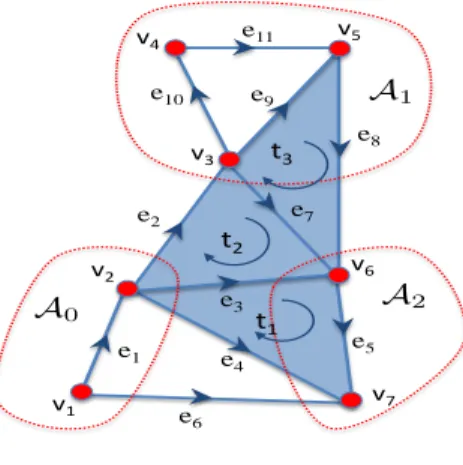
of theflow circulating along the edges of thei-th triangle. As an example for the simplicial complex in Fig. 1, we have
BT2 = 0 0 1 −1 1 0 0 0 0 0 0 0 1 −1 0 0 0 1 0 0 0 0 0 0 0 0 0 0 −1 1 1 0 0 (21) and, defining s1 = [e 1, e2, . . . , e10, e11]T, we get curl(s1) =
[e3−e4+e5, e2−e3+e7,−e7+e8+e9]T. Each entry ofs1
is then the circulation over the corresponding triangle. Similarly, the (discrete) divergence operator maps the edge signals1onto a signal defined over the vertex space, i.e.
RV,
and it is defined as
div(s1) =B1s1. (22)
Again, by direct substitution, it turns out that thei-th entry of div(s1)represents thenet-flow passing through thei-th vertex,
i.e. the difference between the inflow and outflow at node i. Thus a non-zero divergence reveals the presence of a source or sink node. For the example in Fig. 1, we get
B1= −1 0 0 0 0 −1 0 0 0 0 0 1 −1−1−1 0 0 0 0 0 0 0 0 1 0 0 0 0 −1 0 −1−1 0 0 0 0 0 0 0 0 0 0 1 −1 0 0 0 0 0 0 0 −1 1 0 1 0 0 1 0 −1 0 1 1 0 0 0 0 0 0 1 1 1 0 0 0 0 0 (23)
so that div(s1) = [−e
1−e6, e1−e2−e3−e4, e2−e7−e9−
e10, e10−e11,−e8+e9+e11, e3−e5+e7+e8, e4+e5+e6]T.
If we consider equation (19) in the casek= 1,
s1=BT1 s0+s1H+B2s2, (24)
recalling that B1B2 = 0, it is easy to check that the first
component in (24) has zero curl, and then it may be called an irrotationalcomponent, whereas the third component has zero divergence, and then it may be called asolenoidalcomponent, in analogy to the calculus terminology used for vector fields. The harmonic component s1
H is a flow vector that is both
v1 v2 e1 t1 v3 v6 v4 v5 t2 e2 e5 e3 e10 e8 e11 e9 e4 t3 v7 e7 e6
Fig. 1: Cut of order1.
curl-free and divergence-free. Notice also that, in (24),BT1 s0 represents the (discrete)gradient ofs0.
C. Topology-aware unitary basis
In this section, we propose a method to build a unitary basis to represent edge signals, reflecting topological properties of the complex, more specifically triple-wise relations. The idea underlying the method is to search a basis that minimizes a real-valued function capturing triple-wise relations. For example, in the graph case, a key topological property is connectivity, which is well captured by the cutfunction. The associated real-valued function can be built using the so called Lov´asz extension[49], [50] of the cut size. More specifically, given a graphG(V,E)and a partition of its vertex setV in two sets A0 andA1, withA0∪A1=V andA0∩A1=∅, the cut size is defined as
F0(A0,A1) = cut(A0,A1), X i∈A0 X j∈A1 aij (25)
whereaij = 1if(i, j)∈Eandaij= 0otherwise.F0(A0,A1)
is a set function and is known to be a submodular function [49]. Now, we want to translate the set function F0(A0,A1)
onto a real-valued function f0(x0), defined over RV, to be
used for the subsequent optimization. This can be done using the so calledLov´asz extension[49], which is equal to:
f0(x0) = V X i=1 V X j=1 aij|x0i −x 0 j| (26) with x0 ∈
RV. The function in (26) measures the total
variation of a signal defined over the nodes of a graph and then it can be used as a regularization function, whenever the signal of interest is known to be a smooth function. The function in (26) formed the basis of the method proposed in [51] to build a unitary basis for analyzing signals defined over the vertices of a graph. More specifically, in [51] the basis was built by solving the following optimization problem
U,(u1, . . . ,uV) = arg min U∈RV×V V X n=2 f0(un) s.t. UTU=I, u 1= √1V1 (27)
where1is theV×1vector of all ones. In the above problem, the objective function to be minimized is convex, but the problem is non-convex because of the unitarity constraint. To simplify the search for the basis, the objective function in (27) can be relaxed to become
f0r(x0) = V X i=1 V X j=1 aij(x0i −x 0 j) 2. (28)
Substituting (28) in (27), we still have a non-convex problem. However, its solution is known to be given by the eigenvectors of L0. From this perspective, the basis typically used in the
GFT, built as the eigenvectors of the Laplacian matrix, can be interpreted as the solution of the above optimization problem, after relaxation.
Now, we extend the previous approach to find a regularization function capturing triple-wise relations, useful to analyze sig-nals defined over the edges of a graph. In the previous case, the analysis of node signals started from the bi-partition of a graph and then the construction of a real-valued extension of the cut size. Here, to analyze edge signals, we need to start from the tri-partition of the discrete set and define a set function counting the number oftrianglesgluing the three sets together. The function to be minimized should then be the real valued (Lov´asz) extension of such a set function.
The combinatorial study of simplicial complexes has attracted increasing attention and the generalization of Cheeger inequal-ities to simplicial complexes has been the subject of several works [52], [53]. In particular, Hein et al. introduced the total variation on hypergraphs as the Lov´asz extension of the hypergraph cut, defined as the size of the hyperedges set connecting a bipartition of the vertex set [54]. In this work, we derive a Lov´asz extensiondefined over the edge set. More formally, we study a simplicial complexX(V,E,T)of order two, as in the example sketched in Fig.1, and consider the partition of V in three sets (A0,A1,A2). The triple-wise coupling function is now defined as
F1(A0,A1,A2) = X i∈A0 X j∈A1 X i∈A2 aijk (29)
where aijk = 1 if(i, j, k)∈T andaijk = 0otherwise. Our
main result, stated in the following theorem, is that the Lov´asz extension of the triple-wise coupling function gives rise to a measure of the curl of edge signals along triangles.
Theorem1: LetA0,A1,A2be a partition of the vertex set
V of the2-dimensional simplicial complexX(V,E,T)with |E| = E, |T| = T. Then the Lov´asz extension f : RE → R, evaluated at x1 ∈ RE, of the triple-wise coupling size
F1(A0,A1,A2)defined in (29), is f1(x1) = E X i,j,k=1 aijk|x1i −x1j+x1k| = T X j=1 E X i=1 B2(i, j)x1i (30) where B2(i, j) are the edge-triplet incidence coefficients
de-fined in (3).
Proof. Please see Appendix A.
The function in (30) represents the sum of the absolute values of the curls over all the triangles. Differently from [54],
where the total variation over a hypergraph was built from a bipartition of a discrete set and it was a function defined over
RV, in our case, we start from atriparitionof the original set
and we build a real-valued extension, defined overRE, i.e. a
space of dimension equal to the number of edges. A suitable unitary basis for representing (curling) edge signals can then be found as the solution of the following optimization problem
U,(u1, . . . ,uE) = arg min U∈RE×E E X n=1 f1(un) s.t. UTU=I. (31)
The objective function is convex, but the problem is non-convex because of the unitarity constraint. The above problem can be solved resorting to the algorithm proposed in [51], tuned to the new objective function given in (30). Alternatively, similarly to what is typically done with graphs,f1(x1)can be
relaxed and replaced with
f1r(x1) = T X j=1 E X i=1 B2(i, j)x1i !2 =x1TB2BT2x 1. (32) Substituting this function back to (31), the solution is given by the eigenvectors ofB2BT2.
The above arguments show that the eigenvectors ofB2BT2
provide a suitable basis to analyze edge signals having a curling behavior. However, as we know from the Hodge decomposition recalled in the previous section, edge sig-nals contain other useful components that are orthogonal to solenoidal signals, namely irrotational and harmonic compo-nents. Then, in general, it is useful to take as a unitary basis for analyzing edge signalsallthe eigenvectors of L1, i.e. the
eigenvectors associated to the nonzero eigenvalues of B2BT2
and ofBT1B1, plus the eigenvectors associated to the kernel of
L1. In summary, the theory developed in this section provides
a further argument, rooted on intrinsic topological properties of the simplicial complex on which the signal is defined, to exploit the Hodge decomposition to find a suitable basis for the analysis of edge signals. Furthermore, the theory says that using the Laplacian eigenvectors comes as a consequence of a relaxation step. In many cases, whenever the numerical complexity is not an issue, it may be better to keep the `1
-norm objective functions given in (26) and (30), as this would yield more sparse, and then more informative, representations, as a generalization of what done for directed graphs in [51].
IV. EDGE FLOWS ESTIMATION
Let us consider now the observation of an edge signal affected by additive noise. Our goal in this section, is to formu-late the denoising problem as a constrained problem, rooted on the Hodge decomposition. Denoising edge signals embedded in noise was already considered in [42], [31], [32] and, more specifically, in [18]. The formulation proposed in [18] was based on the definition of signals over simplicial complexes as skew-symmetric arrays of dimension equal to the order of the corresponding simplex plus one. So, the edge flow was represented as a matrix (i.e., a two-dimensional array) satisfy-ing the constraintX(i, j) = −X(j, i). A signal defined over
the triangles was represented as an array of dimension three, satisfying the property Φ(i, j, k) = Φ(j, k, i) = Φ(k, i, j) = −Φ(j, i, k) = −Φ(i, k, j) = −Φ(k, j, i). Our aim in this section, is to formulate the denoising optimization problem dealing only with vectors. Based on (19), the observed vector can be modeled as
x1=BT1 s0+s1H+B2s2+v1 (33)
wherev1is noise. Let us suppose, for simplicity, that the noise vector is Gaussian, with zero-mean entries all having the same varianceσn2. The optimal estimator can then be formulated as
the solution of the following problem (ˆs0,ˆs2,sˆ1H) = argmin s0∈RV,s2∈RT,s1 H∈RE kB2s2+B1Ts0+s1H−x 1k2 s.t. B1s1H =0 BT 2s1H =0 (Q). (34) Note that problemQ is convex. Then, there exists multipliers λ1 ∈ RV,λ2 ∈ RT such that the tuple (ˆs0,ˆs2,ˆs1H,λ1,λ2)
satisfies the Karush-Kuhn-Tucker (KKT) conditions ofQ(note that Slater’s constraint qualification is satisfied [55]). The associated Lagrangian function is
L(s0,s2,s1H,λ1,λ2) = (B2s2+BT1s 0+s1 H−x 1)T ·(B2s2+BT1s 0+s1 H−x 1) +λT 1B1s1H+λ T 2B T 2s 1 H. (35) Exploiting the orthogonality propertyB1B2=0, it is easy to
get the following KKT conditions
(a) ∇s0L(s0,s2,s1H,λ1,λ2) =B1BT1s0−B1x1=0 (b) ∇s2L(s0,s2,s1H,λ1,λ2) =BT2B2s2−BT2x 1=0 (c) ∇s1 HL(s 0,s2,s1 H,λ1,λ2) =s1H−x 1+BT 1λ1+B2λ2=0 (d) B1s1H =0, BT2s1H=0 (e) λ1∈RV,λ2∈RT.
Note that conditions (a)-(c) reduce to (a)L0s0=B1x1
(b)BT2B2s2=BT2x 1
(c)s1H =x1−BT1λ1−B2λ2.
(36)
Multiplying both sides of condition (c) byBT
2, and using the
second equality in (d) and condition (b), we get
BT2B2s2=BT2B2λ2. (37)
This means that s2 and λ
2 may differ only by an additive
vector lying in the nullspace ofBT
2B2. Let us sets2=λ2+c2,
withBT
2B2c2=0. Similarly, multiplying (c) byB1and using
the first equality in (d) and condition (a), we obtain
B1BT1s 0=B
1BT1λ1, (38)
which implies thats0=λ1+c1, withc1such thatB1BT1c1=
0. Thus, condition (c) reduces to
s1H=x1−B1Ts0−B2s2 (39)
which says, as expected, that we can derive the harmonic component by subtracting the estimated solenoidal and irrota-tional parts from the observed flow signal x1. To recover the
(a)
(b)
Fig. 2: Observed flow on a simplicial complex (a) and recon-struction of the irrotational flow (b).
irrotational flow s1
irr from the 0-order signal s0 we need to solve equation (a) in (36). Note thatL0 is not invertible. For
connected graphs, it has rankV−1and its kernel is the span of the vector1of all ones. However, since the vectorb=B1x1
is also orthogonal to 1, the normal equation L0s0 = B1x1
admits the nontrivial solution (at least for connected graphs): s0=L†0B1x1
where† denoted the Moore-Penrose pseudo-inverse.
Similarly, the 2-order signal s2, solution of the second
equation in (36), can be obtained as s2= (BT2B2)†BT2x
1
since BT
2x1 is orthogonal to the null space of BT2B2. The
irrotational, solenoidal and harmonic components can then be recovered as follows ˆ s1irr=BT1sˆ 0 =BT1L † 0B1x1 ˆ s1sol=B2ˆs2=B2(BT2B2)†BT2x1 ˆ s1H=x1−sˆ1irr−ˆs1sol. (40)
Note that the first two conditions in (36) imply that the variabless0,s2inQ are indeed decoupled so that the optimal
solutions coincide with those of the following problems ˆ s0= argmin s0∈RV kBT1s0−x1k2 ( Q0) (41) ˆ s2= argmin s2∈RT kB2s2−x1k2 (Q2). (42)
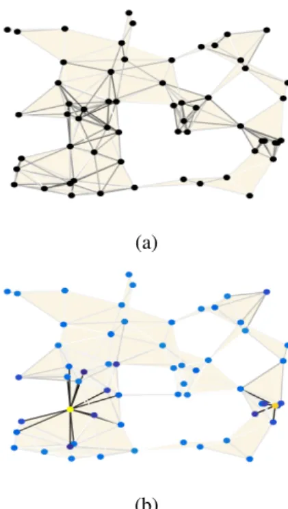
An example of an edge (flow) signal is reported in Fig. 2(a), representing the simulation of data packet flow over a network, including measurement errors. The signal values are encoded in the gray color associated to each link. Suppose now, that
the goal of processing is to detect nodes injecting anomalous traffic in the network, starting from the traffic shown in Fig. 2(a). If some node is a source of an anomalous traffic, that node generates an edge signal with a strong irrotational (or divergence-like) component. To detect spamming nodes, we can then project the overall observed traffic vector s1 onto
the space orthogonal to the space spanned by the nonzero eigenvectors of B2BT2, computing
y1=I−UsolUTsol
s1 (43)
whereUsol is the matrix whose columns collect the eigenvec-tors associated with the nonzero eigenvalues of B2BT2. The
result of this projection is reported in Fig. 2(b), where we can clearly see that the only edges with a significant contributions are the ones located around two nodes, i.e. the source nodes injecting traffic in the network, whose divergence is encoded by the node color.
V. SAMPLING AND RECOVERING OF SIGNAL DEFINED OVER SIMPLICIAL COMPLEX
Suppose now that we only observe a few samples of a k-order signal. The question we address here is to find the conditions to recover the whole signal sk from a subset of samples. To answer this question, we may use the theory developed in [56] for signals on graph, and later extended to hypergraphs in [57]. For simplicity, we focus on signals defined over a simplicial complex of order K = 2, i.e. on vertices, edges and triangles. Given a set of edgesS⊆E we define an edge-limiting operator as a diagonal matrix DS of dimension equal to the number of edges, with a one in the positions where we measure the flow, and zero elsewhere, i.e.
DS=diag{1S} (44) where1S is the set indicator vector whosei-th entry is equal to one if the edge ei∈Sand zero otherwise. We say that an
edge signal s1 is perfectly localized over the subset S ⊆E
(orS-edge-limited) ifs1=D
Ss1. Similarly, given the matrix
U1 whose columns are the eigenvectors of L1, and a subset
of indices F, we define the operator
FF=U1ΣFUT1 (45)
whereΣF=diag(1F). An edge signal s1 isF-bandlimited over a frequency setFifFFs1=s1. The operatorsDSand
FF are self-adjoint and idempotent and represents orthogonal projectors, respectively, on the sets S and F. If we look for edges signals which are perfectly localized in both the edge and frequency domains, some conditions for perfect localization have been derived in [56]. More specifically: a) s1 is perfectly localized over both the edge set S and the
frequency setFif and only if the operator FFDSFFhas an eigenvalue equal to one, i.e.
kDSFFk2=kFFDSk2=kFFDSFFk2= 1 (46)
where kAk2 denotes the spectral norm of A; b) a sufficient
condition for the existence of such signals is that|S|+|F|> E. Conversely, if |S| +|F| ≤ E, there could still exist perfectly localized vectors, when condition (46) holds.
In the following we first consider sampling on a single layer by extracting samples from the edge signals and then, we consider multi-layer processing using samples of signals defined over different layers of the simplex.
A. Single-layer sampling
In the following theorem [56] we provide a necessary and sufficient condition to recover the edge signal s1 from its
sampless1
S,DSs1.
Theorem2: Given the bandlimited edge signals1=F
Fs1,
it is possible to recovers1 from a subset of samples collected
over the subsetS⊆E if and only if the following condition holds:
kD¯SFFk2=kFFD¯Sk2<1 (47)
withD¯S=I−DS.
Proof.The proof is a straightforward extension of Th. 4.1 in [56] to signals defined on the edges of the complex.
In words, the above conditions mean that there can be no F-bandlimited signals that are perfectly localized on the complementary setS¯. Perfect recovery of the signal s1 from s1S can be achieved as
r1=QSsS1 (48) where QS = (I−D¯SFF)−1. The existence of the above inverse is ensured by condition (47). In fact, the reconstruction error can be written as [56]
s1−QSsS1 =s 1−Q
S(I−D¯S)s1=s1−QS(I−D¯SFF)s1=0, where we exploited in the second equality the bandlimited condition s1=F
Fs1.
To make (47) holds true, we must guarantee that
DSFFs1 6= 0 or, equivalently, that the matrix DSFF is full column rank, i.e. rank(DSFF) =|F|. Then, a necessary condition to ensure this holds is|S| ≥ |F|.
An alternative way to retrieve the overall signal s1 from its
samples can be obtained as follows. If (47) holds true, the entire signals1 can be recovered froms1S as follows
s1=UF UTFDSUF −1
UTFs1S (49) where UF is the E × |F| matrix whose columns are the eigenvectors of L1 associated with the frequency setF. Remark: It is worth to notice that, because of the Hodge decomposition (18), an edge signal always contains three components that are typically band-limited, as they reside on a subspace of dimension smaller than E. This means that, if one knowsa priori, that the edge signal contains only one component, e.g. solenoidal, irrotational, or harmonic, then it is possible to observe the edge signal and to recover the desired component over all the edges, under the conditions established by Theorem 2.
B. Multi-layer sampling
In this section, we consider the case where we take samples of signals of different order and we propose two alternative strategies to retrieve an edge signals1 from these samples. The first approach aims at recovering s1 by using both, the vertex signal sampless0
sampless1
S=DSs1. Hereinafter, we denote byFirr,Fsoland
FH the set of frequency indexes in F corresponding to the eigenvectors ofL1belonging, respectively, to the irrotational,
solenoidal and harmonic subspaces. Note that, if s1 is F
-bandlimited then also s1
H, s1sol and s1irr are bandlimited with bandwidth, respectively,|FH|,|Fsol|and|Firr|. DefineFsH as the set of frequency indexes such thatFsH=FH∪Fsol. Fur-thermore, given the matrixU0with columns the eigenvectors
of L0, we define the operator F0F0 =U0ΣF0U
T
0 where|F0|
denotes the bandwidth of s0. Let C1 be the set of indexes in F0 associated with the eigenvectors belonging to ker(L0)
and denote by U0F0−C1 the matrix whose columns are the eigenvectors ofL0associated with the frequency setF0−C1.
Then, we can state the following theorem.
Theorem 3: Consider the second-order simplex
X(V,E,T) and the edge signal s1 = s1sol +s1H +BT1s0.
Then, assume that: i) the vertex-signals0and the edge signal s1 are bandlimited with bandwidth, respectively, |
F0| and
|F| = |FsH|+|F0| −c1, where |FsH| =|Fsol|+|FH| and
c1 ≥0 denotes the number of eigenvectors in the bandwidth
ofs0belonging to ker(L
0); ii) the conditionskD¯AF0F0k2<1 and kD¯SFFsHk2<1 hold true. Then, it follows that:
a) s1 can be perfectly recovered from both a set of vertex signal samples s0A =DAs0 and from the edge samples s1S=DSs1 via the set of equations
" s0 ¯ s1 # =Q " s0A sS1 # , (50) where ¯s1=s1sol+s1H, Q= " (I−DAF0F0) −1 O P (I−DSFFsH) −1 # (51) and P=−(I−DSFFsH) −1D SBT1F 0 F0(I−DAF 0 F0) −1;
b) There exists a set of frequency indexes Firr ⊂ F, for
which the eigenvectors matrix UFirr of L1 satisfies the
equality UFirr = B T
1U 0
F0−C1, and such that any F -bandlimited edge signal with set of frequency indexes
F=Firr∪FsHand |Firr|=|F0| −c1 can be recovered
by using N0 ≥ |F0| samples from s0 and N1 ≥ |FsH|
samples from s1.
Proof. See the supporting material in [58, Appendix B]. Let us now consider the case where we want to recover s1 from samples collected from signals of order0,1, and 2,
i.e. s0, s1 and s2. We denote by s2
M = DMs2 the vector of triangle signal samples with M ⊆T. Furthermore, given the matrix U2 with columns the eigenvectors of the
second-order LaplacianL2, we define the operatorF2F2 =U2ΣF2U
T
2
where |F2| denotes the bandwidth ofs2. Then, assumings2
bandlimited, it holds s2=F2F2s2. Denote withC2 the set of indexes in F2 associated with the eigenvectors belonging to
ker(L2)and with U2F2−C2 the matrix whose columns are the eigenvectors of L2 associated with the index setF2−C2.
Theorem 4: Consider the second-order simplex
X(V,E,T), the edge signal s1 = B2s2 +s1H +B T
1s0
and assume that: i) the vertex-signal s0, the edge signal s1 and the triangle signal s2 are bandlimited with bandwidth,
respectively,|F0|,|F1|=|F0|+|FH|+|F2| −(c1+c2)and
|F2|, with c1 ≥ 0 and c2 ≥ 0 the number of eigenvectors
in the bandwidth of s0 and s2 belonging, respectively, to
ker(L0) and ker(L2); ii) all conditions kD¯AF0F0k2 < 1, kD¯SFFHk2 < 1 and kD¯MF
2
F2k2 < 1 hold true. Then, it follows:
a) s1 can be perfectly recovered from a set of vertex signal sampless0A=DAs0, from the edge sampless1S=DSs1
and from the triangle sampless2M=DMs2as s0 s1 H s2 =R s0 A s1 S s2 M , (52) where R= (I−DAF0F0) −1 O O P1 P2 P3 O O (I−DMF2F2) −1 (53) andP1=−(I−DSFFH) −1D SBT1F 0 F0(I−DAF 0 F0) −1, P2 = (I − DSFFH) −1, P 3 = −(I − DSFFH) −1D SB2F2F2(I−DMF 2 F2) −1;
b) There exist two sets of frequency indexesFsol,Firr⊂F,
for which the eigenvectors ofL1stacked in the columns of
the matricesUFsol,UFirr satisfy, respectively, the equality
UFsol = B2U 2 F2−C2, and UFirr = B T 1U 0 F0−C1. Then, anyF-bandlimited edge signal with frequency set F=
Fsol∪Firr∪FH, and|Firr|=|F0|−c1,|Fsol|=|F2|−c2,
can be recovered by using N0≥ |F0| samples from s0,
N1 ≥ |FH| samples from s1 and N2 ≥ |F2| samples
froms2.
Proof.See the supporting material in [58, Appendix B]. VI. ESTIMATION OF DISCRETE VECTOR FIELDS
Developing tools to process signals defined over simplicial complexes is also useful to devise algorithms for processing discrete vector fields. The use of algebraic topology, and more specificallyDiscrete Exterior Calculus(DEC), has been already considered for the analysis of vector fields, especially in the field of computer graphic. Exterior Calculus (EC) is a discipline that generalizes vector calculus to smooth manifolds of arbitrary dimensions [59] and DEC is a discretization of EC on simplicial complexes [60], [61]. DEC methodologies have been already proposed in [62] to produce smooth tangent vec-tor fields in computer graphics. Smoothing tangential vecvec-tor fields using techniques based on the spectral decomposition of higher order Laplacian was also advocated in [63]. In this section, building on the basic ideas of [62], [63], we propose an alternative approach to smooth discrete vector fields. More specifically, as in [62], [63], the proposed approach is based on three main steps: i) map the vector field onto an edge signal; ii) filter the edge signal; and iii) map the edge signal back to a vector field. Steps i) and iii) are essentially the same as in [63]. The difference we introduce here is in step ii), i.e. in the filtering of the edge signal. Filtering edge signals has been considered before, see, e.g., [32], but in our case we consider a
different formulation and we incorporate the proper metrics in the Hodge Laplacian, dictated from the initial mapping from the vector field to the corresponding edge signal.
To filter vector fields, we need first to embed the vector field and the simplicial complex into a real space. Let us denote with X a simplicial complex embedded in a real space Rn
of dimension n. We assume that X is flat, i.e. all simplices are in the same affine n-subspace, and well-centered, which means the circumcenter of each simplex lies in its interior [60]. A discrete vector field ~v can be considered as a map from pointsxi ofX toRn. An illustrative example is shown
in Fig. 3(a), where the discrete vector field is represented by the set of arrows associated to the points in a regular grid in
R2. In many applications, it is of interest to develop tools to
extract relevant information from a vector field or to reduce the effect of noise. Our proposed approach is based on the following three main steps:
1) Map a vector field onto a simplicial complex signal Given the set ofN pointsxi, we build the simplicial complex
X using a well-centered Delaunay triangulation with vertices (0-simplicies) in the pointsxi[60]. Then, starting from the set
of vectors~v(xi), we recover a continuous vector field through
interpolation based on the Whitney basis functionsφi(x)[64]
~v(x) = N X i=1 ~ v(xi)φi(x) (54)
whereφi(x)are affine piecewise functions. More specifically,
φiis an hat function on vertexvi, which takes on the value one
at vertex vi, i.e. φi(xi) = 1, is zero at all other vertices, and
affine over each 2-simplex havingvi as vertex. Then, project
the vector field onto the set of1-simplices (edges), giving rise to a set of scalar signals defined over the edges of the complex
x1j = ~v(σ 0 j0) +~v(σ 0 j1) 2 ! ·~σ1j, j= 1, . . . , E (55)
where j0 andj1 are the end-points of edge j and~σ1j stands
for the vector corresponding to σ1
j = [σ0j0, σ
0
j1], having the same direction as the orientation of σ1
j. The vector x1∈RE
of edge signals associated with the vector field~v, is then built as x1= [x1
1, . . . , x1E] T.
2) Filter the signal defined on the simplicial complex The filtering strategy aims to recover an edge flow vectors1
that fits the observed vector x1, it is smooth and sparse. We
recover the vector s1 as the solution of
min s1∈RE ks
1−x1k
2+λs1TL1s1+γks1k1 (PF) where λ, γ are positive penalty coefficients controlling, re-spectively, the signal smoothness and its sparsity. Since we chose the Whitney form as interpolation basis, for any two signals of order p, xp,yp ∈
RNp, the induced inner product
is given by xpTM
pyp, where the Np × Np-dimensional
matrixMp, incorporating the Whitney metric, is derived as in
[61][Prop. 9.7]. Therefore, the Hodge LaplacianL1, weighted
with the appropriate metric matricesMp, withp= 0,1,2, is
a semidefinite positive matrix that can be written as
L1=B2M2BT2 +M1BT1M
−1
0 B1M1 (56)
Observed RNA velocity field
(a)
Noisy RNA velocity field
(b)
Filtered RNA velocity field
(c)
Fig. 3: RNA velocity fields: (a) observed and (b) noisy fields; (c) reconstructed field.
while the fitting error norm becomes
ks1−x1k2= (s1−x1)TM1(s1−x1). (57)
3) Map the filtered signal back onto a discrete vector field Finally, given the discrete signal of order 1, s1eij, ∀eij ∈E,
the generated piecewise linear vector field becomes [62] ~
v(x) =X
eij
s1e
ij[φi(x)∇φj(x)−φj(x)∇φi(x)]. (58)
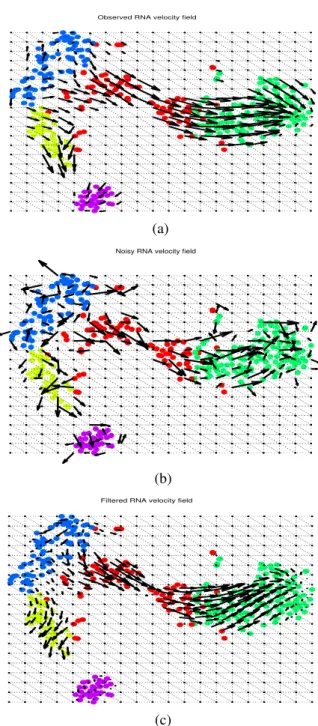
We show now an interesting application of the above pro-cedure to the analysis of the vector field representing the RNA velocity field, defined as the time derivative of the gene expression state [41], useful to predict the future state
of individual cells and then the direction of change of the entire transcriptome during the RNA sequencing dynamic process. The RNA velocity can be estimated by distinguishing between nascent (unspliced) and mature (spliced) messenger RNA (mRNA) in common single-cell RNA sequencing pro-tocols [41]. We consider the mRNA-seq dataset of mouse chromaffin cell differentation analysed in [41]. An example of RNA velocity vector field is illustrated in Fig. 3(a). To analyze such a vector field using the proposed algorithms, we implemented steps 1) and 3) using the discrete exterior calculus operators provided by the PyDEC software developed in [61]. We considered a Delaunay well-centered triangulation of the continuous bi-dimensional space, which generates the simplicial complexes in Fig. 3 composed ofN = 400nodes, where we fill all the triangles. The velocity field in Fig. 3(a) is observed over156 vertices and the field vector at each vertex has been obtained with a local Gaussian kernel smoothing [41]. The underlying colored cells represented different states of the cell differentiation process. Then, to test our filtering strategy, we added a strong Gaussian noise to the observed velocity field, with SNR= 0dB, as illustrated in Fig. 3(b). This noise is added to incorporate mRNA molecules degradation and model inaccuracy. Then we apply the proposed filtering strategy by first reconstructing the edge signal as in (54) and then recovering the edge signal as a solution of the optimization problemPF. Finally, we reconstruct the vector field using the interpolation formula (58), observed at the barycentric points of each triangles. The result is reported in Fig. 3(c), where we can appreciate the robustness of the proposed filtering strategy.
VII. INFERENCE OF SIMPLICIAL COMPLEX TOPOLOGY FROM DATA
The inference of the graph topology from (node) signals is a problem that has received significant attention, as shown in the recent tutorial papers [65], [39], [40] and in the references therein. In this section, we propose algorithms to infer the structure of a simplicial complex. Given the layer structure of a simplicial complex, we propose a hierarchicalapproach that infers the structure of one layer, assuming knowledge of the lower order layers. For simplicity, we focus on the inference of a complex of order 2 from the observation of a set of M edge (flow) signals X1 :=
x1(1), . . . ,x1(M)
, assuming that the topology of the underlying graph is given (or it has been estimated). So, we start from the knowledge of
L0, which implies, after selection of an orientation, knowledge
of B1. SinceL1=B1TB1+B2BT2, then we need to estimate
B2. Before doing that, we check, from the data, if the term
B2BT2 is really needed. Since, from (24), the only components
that may depend on B2 are the solenoidal and harmonic
components, we first project the observed flow signal onto the space orthogonal to the space spanned by the irrotational component, by computing
x1sH(m) = I−UirrUTirr
x1(m), m= 1, . . . , M, (59) whereUirr is the matrix whose columns are the eigenvectors associated with the nonzero eigenvalues of BT1B1. Then,
denoting withX1sH= x1 sH(1), . . . ,x 1 sH(M)
the signal matrix
of size E×M, we measure the energy ofX1sH by taking its normkX1sHkF: If the norm is smaller than a thresholdηof the
averaged energy of the observed data set, we stop, otherwise we proceed to estimateB2.
The first step in the estimation of B2 starts from the
detection of all cliques of three elements present in the graph. Their number isT = traceh(L0−diag(L01))
3i
/6. For each clique, we choose, arbitrarily, an orientation for the potential triangle filling it. The matrixB2 can then be written as
B2=
T X
n=1
tnbnbTn (60)
where bn is the vector of size E associated with the n-th
clique, whose entries are all zero except the three entries associated with the three edges of the n-th clique. Those entries assume the value1or−1, depending on the orientation of the triangle associated with then-th clique. The coefficients tn in (60) are equal to one, if there is a (filled) triangle on
the n-th clique, or zero otherwise. The goal of our inference algorithm is then to decide, starting from the data, which entries of t := [t1, . . . , tT] are equal to one or zero. Our
strategy is to make the association that enforces a small total variation of the observed flow signal on the inferred complex, using (32) as a measure of total variation on flow signals. We propose two alternative algorithms: The first method infers the structure of B2 by minimizing the total variation of the
observed data; the second method performs first a Principal Component Analysis (PCA) and then looks for the matrix
B2 and the coefficients of the expansion over the principal
components that minimize the total variation plus a penalty on the model fitting error.
Minimum Total Variation (MTV) Algorithm: The goal of
this algorithm is to minimize the total variation over the observed data set, assuming knowledge of the number of triangles. The set of coefficientst is found as solution of
min t∈{0,1}T q(t), T X n=1 tntrace X1sHTbnbTnX 1 sH (PMTV) s.t. ktk0=t∗, tn ∈ {0,1},∀n, (61) where t∗ is the number of triangles that we aim to detect. In practice, this number is not known, so it has to be found through cross-validation. Even though problemPMTV is non-convex, it can be solved in closed form. Introducing the nonnegative coefficientscn =P
M i=1x
1T
sH (i)bnbTnx1sH(i), the solution can in fact be obtained by sorting the coefficientscn
in increasing order and then selecting the triangles associated with the indices of the t∗ lowest coefficients cn. Note that
the proposed strategy infers the presence of triangles along the cliques having the minimum curl along its edges. Hence, we expect better performance when the edge signal contains only the harmonic components, whose curls along the filled triangles is exactly null.
PCA-based Best Fitting with Minimum Total Variation (PCA-BFMTV): To robustify the MTV algorithm in the case where the edge signal contains also a solenoidal component and is possibly corrupted by noise, we propose now the
PCA-BFMTV algorithm that infers the structure of B2 and the
edge signal that best fits the observed data set X1, while at the same time exhibiting a small total variation over the inferred topology. The method starts performing a principal component analysis of the observed data by extracting the eigenvectors associated with the largest eigenvalues of the covariance matrix estimated from the observed data set. More specifically, the proposed strategy is composed of two steps: 1) estimate the covariance matrix CbX from the edge signal
data set X1sH and builds the matrix UbsH whose columns are the eigenvectors associated with the F largest eigenvalues of
b
CX; 2) model the observed data set as X1sH = UbsHSb 1
sH and searches for the coefficient matrix bS
1
sH and the vector t that solve the following problem
min t∈{0,1}T,Sb 1 sH∈RF×M g(t,bS 1 sH) +γkX 1 sH−UbsHSb 1 sHk2F s.t. ktk0=t∗, tn∈ {0,1},∀n, (PTS) (62) whereg(t,Sb 1 sH), T X n=1 tntrace(bS 1T sH UbTsHbnbTnUbsHbS 1 sH)andγ is a non-negative coefficient controlling the trade-off between the data fitting error and the signal smoothness. Although problem PTS is non-convex, it can be solved using an iter-ative alternating optimization algorithm returning successive estimates of Sb
1
sH, having fixed t, and alternately t, given
b
S1sH. Interestingly, each step of the alternating optimization problem admits a closed form solution. More specifically, at each iterationk, the coefficient matrixbS
1 sH[k]can be found as b S1sH[k] = arg min b S1sH∈RF×M g(t[k],bS 1 sH) +γkX 1 sH−UbsHSb 1 sHk2F (PSk). Defining Lupp[k] := P T n=1tn[k]bnbTn, problem PSk admits the closed form solution
b
SsH1 [k] = (IF +γUbTsHLupp[k]UbsH)−1UbTsHX1sH. (63)
Then, given bS 1
sH[k], we can find the vector t[k+ 1]using the same method used to solve problem MTV, in (61), i.e. setting cn[k] := trace(Sb
1
sH[k]TUbTsHbnbTnUbsHbS 1
sH[k]) and taking the entries of tn[k+ 1] equal to1 for the indices corresponding
to the first t∗ smallest coefficients of {cn[k]}Tn=1, and 0
otherwise. The iterative steps of the proposed strategy are reported in the box entitled Algorithm PCA-BFMTV. Now we test the validity of our inference algorithms over both simulated and real data.
Performance on synthetic data: Some of the most critical parameters affecting the goodness of the proposed algorithms are the dimension of the subspaces associated with the solenoidal and harmonic components of the signal and the number of filled triangles in the complex. In fact, in both MTV and PCA-BFMTV a key aspect is the detection of triangles as the cliques where the associated curl is minimum. Hence, if the signal contains only the harmonic component and there is no noise, the triangles can be identified with no error, because the harmonic component is null over the filled triangles.
Algorithm PCA-BFMTV Setγ >0,t[0]∈ {0,1}T ,kt[0]k0=t∗, Lupp[0] = T X n=1 tn[0]bnbTn,k= 1 Repeat SetbS 1 sH[k] = (IF +γUbTsHLupp[k−1]UbsH)−1UbTsHX1sH;
Computet[k]by sorting the coefficients cn[k] =trace(bS
1
sH[k]TUbTsHbnbTnUbsHSb
1 sH[k]),
and setting to1the entries oft[k]corresponding to thet∗ smallest coefficients, and0otherwise;
Setk=k+ 1, until convergence. −5 0 5 10 15 20 0 0.05 0.1 0.15 0.2 0.25 0.3 0.35 SNR[dB] Pe MTV PCA-BFMTV noiseless MTV (a) −5 0 5 10 15 20 25 30 0 0.05 0.1 0.15 0.2 0.25 0.3 0.35 0.4 0.45 SNR[dB] Pe MTV,|Fsol|= 80 PCA-BFMTV,|Fsol|= 80 noiseless MTV,|Fsol|= 80 MTV,|Fsol|= 10 PCA-BFMTV,|Fsol|= 10 noiseless MTV,|Fsol|= 10 (b)
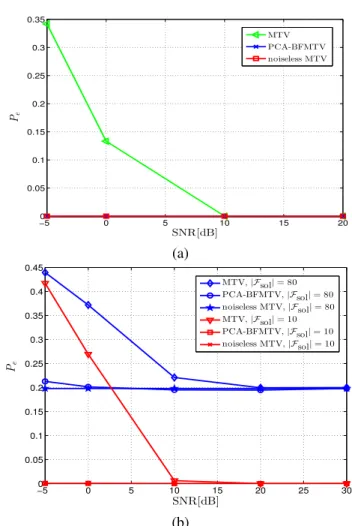
Fig. 4: Error probability by observing: (a) harmonic noisy signals;(b)harmonic plus solenoidal noisy signals.
However, when there is a solenoidal component or noise, there might be decision errors. To test the inference capabilities of the proposed methods, in Fig. 4(a), we report the triangle error probability Pe, defined as the percentage of incorrectly
estimated triangles with respect to the number of cliques with three edges in the simplex, versus the signal-to-noise ratio (SNR), when the observation contains only harmonic flows plus noise. We considered a simplex composed of N = 50 nodes and with a percentage of filled triangles with respect to the number of second order cliques in the graph equal to 50%. We also set M = 50, t∗ = 105 and averaged our numerical results over103zero-mean signal and noise random
realizations. The harmonic signal bandwidth |FH| is chosen
equal to 105, which is equal to the dimension of the kernel of L1. From Fig. 4(a), we can notice, as expected, that in the
noiseless case the error probability is zero, since observing only harmonic flows enables perfect recovery of the matrix
B2. In the presence of noise, the MTV algorithm suffers and
in fact we observe a non negligible error probability at low SNR. However, applying the PCA-BFMTV algorithm enables a significant recovery of performance, as evidenced by the blue curve that is entirely superimposed to the red curve, at least for the SNR values shown in the figure. In this example, the covariance matrix was estimated over 105 independent observations of the edge signals. The optimal γ coefficient was chosen after a cross validation operation following a line search approach aimed to minimize the error probability. The improvement of the PCA-BFMTV method with respect to the MTV method is due to the denoising made possible by the projection of the observed signal onto the space spanned by the eigenvectors associated with the largest eigenvalues of the estimated covariance matrix.
To test the proposed methods in the case where the observed signal contains both the solenoidal and harmonic components, in Fig. 4(b) we reportPeversus the SNR, for different values
of the dimension of the subspace associated with the solenoidal part, indicated as |Fsol|. From Fig. 4(b), we can observe that the performance of both algorithms MTV and PCA-BFMTV suffers when the bandwidth |Fsol| of the solenoidal compo-nent is large, whereas the performance degradation becomes negligible when |Fsol| is small. In all cases, PCA-BFMTV significantly outperforms the MTV algorithm, especially at low SNR values, because of its superior noise attenuation capabilities. As further numerical test, we run algorithm Pk
S replacing the quadratic regularization term with the triple-wise coupling regularization function in (30), by obtaining the same performance of the PCA-BFMTV algorithm.
Performance on real data: The real data set we used to test our algorithms is the set of mobile phone calls collected in the city of Milan, Italy, by Telecom Italia, in the context of the Telecom Big Data Challenge [66]. The data are associated with a regular two-dimensional grid, composed of100×100points, superimposed to the city. Every point in the grid represents a square, of size 235 meters. In particular, the data set collects the number Nij of calls from node i to areaj, as a function
of time. There is an edge between nodes iandj only if there is a non null traffic between those points. The traffic has been aggregated in time, over time intervals of one hour. We define the flow signal over edge (i, j)as Φij =Nij−Nji. We map
all the values of matrixΦinto a vector of flow signalsx1. We
observed the calls daily traffic during the month of December 2013. The data are aggregated for each day over an interval of one hour. Our first objective is to show whether there is an advantage in associating to the observed data setX1a complex of order 2, i.e. a set of triangles, or it is sufficient to use a purely graph-based approach. In both cases, we rely on the same graph structure, whoseB1comes from the data set, after
an arbitrary choice of the edges’ orientation. If we use a graph-based approach, we can build a basis of the observed flow signals using the eigenvectors of the so called edge Laplacian
in [35], i.e. Llow1 = BT1B1. We call this basis Ulow1 . As an
alternative, our proposed approach is to build a basis using the eigenvectors ofL1=BT1B1+B2BT2, whereB2 is estimated
from the data set X1 using our MTV algorithm. We call this basis U1. To test the relative benefits of using U1 as
opposed to Ulow1 , we run a basis pursuit algorithm with the goal of finding a good trade-off between the sparsity of the representation and the fitting error. More specifically, for any given observed vector x1(m), we look for the sparse vector s1 as solution of the following basis pursuit problem [67]:
min s1∈RE ks 1k 1 (B) s.t. kx1−Vs1k F≤ (64)
where V =U1 in our case, while V =Ulow1 in the
graph-based approach. As a numerical result, in Fig. 5 we report the sparsity of the recovered edge signals versus the mean estima-tion errorkx1−Vs1k
F considering as signal dictionaryV
the eigenvectors of either the first-order Laplacian or the lower Laplacian. We used the MTV algorithm to infer the upper Laplacian matrix by setting the numbert∗ of triangles that we may detect equal to 800. This value is derived numerically through cross-validation over a training data set, by choosing the value of t∗ that yields the minimum norm k s1 k
1. As
can be observed from Fig. 5, using the set of the eigenvectors of L1 yields a much smaller MSE, for a given sparsity or,
conversely, a much more sparse representation, for a given MSE. An intuitive reason why our method performs so much better than a purely graph-based approach is that the matrix
L1 has a much reduced kernel space with respect toLlow1 and
the basis built onL1captures much better some inner structure
present in the data by inferring the structure of the additional term B2 from the data itself.
As a further test, we tested the two basis U1 andUlow1 in
terms of the capability to recover the entire flow signal from a subset of samples. To this end, we exploit the band-limited property enforced by the sparse representation, enabling the use of the theory developed in Section V.A. Starting with the representation of each input vector x1 as x1 = Vs1, with
eitherV=U1 in our case, orV=Ulow1 in the graph-based
approach, we used the Max-Det greedy sampling strategy in [56] to select the subset of edges where to sample the flow signal and then we used the recovery rule in (49) to retrieve the overall flow signal from the samples. The numerical results are reported in Fig. 6, representing the normalized recovering error of the edge signal versus the number Ns of samples used to
reconstruct the overall signal. We can notice how introducing the termB2BT2, we can achieve a much smaller error, for the
same number of samples.
VIII. CONCLUSION
In this paper we have presented an algebraic framework to analyze signals residing over a simplicial complex. In particular, we focused on signals defined over the edges of a complex of order two, i.e. including triangles, and we showed that exploiting the full algebraic structure of this complex provides an advantage with respect to graph-based tools only. We have not analyzed higher order signals. Nevertheless,