L
p-Nested Symmetric Distributions
Fabian Sinz [email protected]
Matthias Bethge [email protected]
Werner Reichardt Center for Integrative Neuroscience Bernstein Center for Computational Neuroscience Max Planck Institute for Biological Cybernetics Spemannstraße 41, 72076 T¨ubingen, Germany
Editor: Aapo Hyv¨arinen
Abstract
In this paper, we introduce a new family of probability densities called Lp-nested symmetric
distri-butions. The common property, shared by all members of the new class, is the same functional form ρ(xxx) =ρ˜(f(xxx)), where f is a nested cascade of Lp-normskxxxkp= (∑|xi|p)1/p. Lp-nested symmetric
distributions thereby are a special case ofν-spherical distributions for which f is only required to be positively homogeneous of degree one. While both,ν-spherical and Lp-nested symmetric
dis-tributions, contain many widely used families of probability models such as the Gaussian, spher-ically and elliptspher-ically symmetric distributions, Lp-spherically symmetric distributions, and certain
types of independent component analysis (ICA) and independent subspace analysis (ISA) models,
ν-spherical distributions are usually computationally intractable. Here we demonstrate that Lp
-nested symmetric distributions are still computationally feasible by deriving an analytic expression for its normalization constant, gradients for maximum likelihood estimation, analytic expressions for certain types of marginals, as well as an exact and efficient sampling algorithm. We discuss the tight links of Lp-nested symmetric distributions to well known machine learning methods such
as ICA, ISA and mixed norm regularizers, and introduce the nested radial factorization algorithm (NRF), which is a form of non-linear ICA that transforms any linearly mixed, non-factorial Lp
-nested symmetric source into statistically independent signals. As a corollary, we also introduce the uniform distribution on the Lp-nested unit sphere.
Keywords: parametric density model, symmetric distribution,ν-spherical distributions, non-linear
independent component analysis, independent subspace analysis, robust Bayesian inference, mixed norm density model, uniform distributions on mixed norm spheres, nested radial factorization
1. Introduction
samples for different models. Additionally, such models often allow for a direct optimization of the likelihood.
One way of imposing structure on probability distributions is to fix the general form of the iso-density contour lines. This approach was taken by Fernandez et al. (1995). They modeled the contour lines by the level sets of a positively homogeneous function of degree one, that is functions
νthat fulfillν(a·xxx) =a·ν(xxx)for xxx∈Rnand a∈R+
0. The resulting class ofν-spherical distributions have the general formρ(xxx) =ρ(ν(˜ xxx))for an appropriate ˜ρwhich causesρ(xxx) to integrate to one. Since the only access ofρto xxx is viaνone can show that, for a fixedν, those distributions are gen-erated by a univariate radial distribution. In other words,ν-spherically distributed random variables can be represented as a product of two independent random variables: one positive radial variable and another variable which is uniform on the 1-level set of ν. This property makes this class of distributions easy to fit to data since the maximum likelihood procedure can be carried out on the univariate radial distribution instead of the joint density. Unfortunately, deriving the normalization constant for the joint distribution in the general case is intractable because it depends on the surface area of those level sets which can usually not be computed analytically.
Known tractable subclasses ofν-spherical distributions are the Gaussian, elliptically contoured, and Lp-spherical distributions. The Gaussian is a special case of elliptically contoured distributions. After centering and whitening xxx :=C−1/2(sss−E[sss])a Gaussian distribution is spherically symmetric and the squared L2-norm||xxx||22=x21+· · ·+x2nof the samples follow aχ2-distribution (that is, the radial distribution is aχ-distribution). Elliptically contoured distributions other than the Gaussian are obtained by using a radial distribution different from the χ-distribution (Kelker, 1970; Fang et al., 1990).
The extension from to Lp-spherically symmetric distributions is based on replacing the L2-norm by the Lp-norm
ν(xxx) =kxxxkp= n
∑
i=1
|xi|p
!1
p
,p>0
in the density definition. That is, the density of Lp-spherically symmetric distributions can always be written in the formρ(xxx) =ρ(˜ ||xxx||p). Those distributions have been studied by Osiewalski and Steel (1993) and Gupta and Song (1997). We will adopt the naming convention of Gupta and Song (1997) and callkxxxkp an Lp-norm even though the triangle inequality only holds for p≥1.
Lp-spherically symmetric distributions with p6=2 are no longer invariant with respect to rotations (transformations from SO(n)). Instead, they are only invariant under permutations of the coordinate axes. In some cases, it may not be too restrictive to assume permutation or even rotational symmetry for the data. In other cases, such symmetry assumptions might not be justified and cause the model to miss important regularities.
the cascade. As demonstrated in Sinz et al. (2009b), one possible application domain of Lp-nested symmetric distributions is natural image patches. In the current paper, we would like to present a formal treatment of this class of distributions. Readers interested in the application of these distri-butions to natural images should refer to Sinz et al. (2009b).
We demonstrate below that the construction of the nested Lp-norm cascade still bears enough structure to compute the Jacobian of polar-like coordinates similar to those of Song and Gupta (1997), and Gupta and Song (1997). With this Jacobian at hand it is possible to compute the uni-variate radial distribution for an arbitrary Lp-nested symmetric density and to define the uniform distribution on the Lp-nested unit sphereLν={xxx∈Rn|ν(xxx) =1}. Furthermore, we compute the surface area of the Lp-nested unit sphere and, therefore, the general normalization constant for
Lp-nested symmetric distributions. By deriving these general relations for the class of Lp-nested symmetric distributions we have determined a new class of tractableν-spherical distributions which is so far the only one containing the Gaussian, elliptically contoured, and Lp-spherical distributions as special cases.
Lp-spherically symmetric distributions have been used in various contexts in statistics and ma-chine learning. Many results carry over to Lp-nested symmetric distributions which allow a wider application range. Osiewalski and Steel (1993) showed that the posterior on the location of a Lp-spherically symmetric distributions together with an improper Jeffrey’s prior on the scale does not depend on the particular type of Lp-spherically symmetric distribution used. Below, we show that this results carries over to Lp-nested symmetric distributions. This means that we can robustly determine the location parameter by Bayesian inference for a very large class of distributions.
A large class of machine learning algorithms can be written as an optimization problem on the sum of a regularizer and a loss function. For certain regularizers and loss functions, like the sparse L1 regularizer and the mean squared loss, the optimization problem can be seen as the maximum a pos-teriori (MAP) estimate of a stochastic model in which the prior and the likelihood are the negative exponentiated regularizer and loss terms. Sinceρ(xxx)∝exp(−||xxx||pp)is an Lp-spherically symmet-ric model, regularizers which can be written in terms of a norm have a tight link to Lp-spherically symmetric distributions. In an analogous way, Lp-nested symmetric distributions exhibit a tight link to mixed-norm regularizers which have recently gained increasing interest in the machine learn-ing community (see, e.g., Zhao et al., 2008; Yuan and Lin, 2006; Kowalski et al., 2008). Lp-nested symmetric distributions can be used for a Bayesian treatment of mixed-norm regularized algorithms. Furthermore, they can be used to understand the prior assumptions made by such regularizers. Be-low we discuss an implicit dependence assumption between the regularized variables that folBe-lows from the theory of Lp-nested symmetric distributions.
Finally, the only factorial Lp-spherically symmetric distribution (Sinz et al., 2009a), the p-generalized Normal distribution, has been used as an ICA model in which the marginals follow an exponential power distribution. This class of ICA is particularly suited for natural signals like images and sounds (Lee and Lewicki, 2000; Zhang et al., 2004; Lewicki, 2002). Interestingly, Lp -spherically symmetric distributions other than the p-generalized Normal give rise to a non-linear ICA algorithm called radial Gaussianization for p=2 (Lyu and Simoncelli, 2009) or radial factor-ization for arbitrary p (Sinz and Bethge, 2009). As discussed below, Lp-nested symmetric distribu-tions are a natural extension of the linear Lp-spherically symmetric ICA algorithm to ISA, and give rise to a more general non-linear ICA algorithm in the spirit of radial factorization.
for the determinant of the Jacobian for this coordinate transformation. Using this expression, we define the uniform distribution on the Lp-nested unit sphere and the class of Lp-nested symmetric distributions for an arbitrary Lp-nested function in Section 3. In Section 4 we derive an analytical form of Lp-nested symmetric distributions when marginalizing out lower levels of the Lp-nested cascade and demonstrate that marginals of Lp-nested symmetric distributions are not necessarily
Lp-nested symmetric. Additionally, we demonstrate that the only factorial Lp-nested symmetric distribution is necessarily Lp-spherically symmetric and discuss the implications of this result for mixed norm regularizers. In Section 5 we propose an algorithm for fitting arbitrary Lp-nested sym-metric models. We derive a sampling scheme for arbitrary Lp-nested symmetric distributions in Section 6. In Section 7 we generalize a result by Osiewalski and Steel (1993) on robust Bayesian inference on the location parameter to Lp-nested symmetric distributions. In Section 8 we discuss the relationship of Lp-nested symmetric distributions to ICA and ISA, and their possible role as priors on hidden variables in over-complete linear models. Finally, we derive a non-linear ICA al-gorithm for linearly mixed non-factorial Lp-nested symmetric sources in Section 9 which we call nested radial factorization (NRF).
2. Lp-nested Functions, Coordinate Transformation and Jacobian
Consider the function
f(xxx) =|x1|p/0+ (|x2|p1+|x3|p1)
p/0 p1
1
p/0
(1)
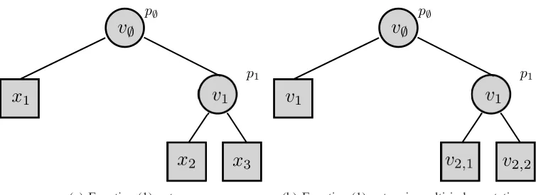
with p/0,p1 ∈R+. This function is obviously a cascade of two Lp-norms and is thus positively homogeneous of degree one. Figure 1(a) shows this function visualized as a tree. Naturally, any tree like the ones in Figure 1 corresponds to a function of the kind of Equation (1). In general, the n leaves of the tree correspond to the n coefficients of the vector xxx∈Rnand each inner node computes the Lp-norm of its children using its specific p. We call the class of functions which is generated in this way Lp-nested and the corresponding distributions, which are symmetric or invariant with
respect to it, Lp-nested symmetric distributions.
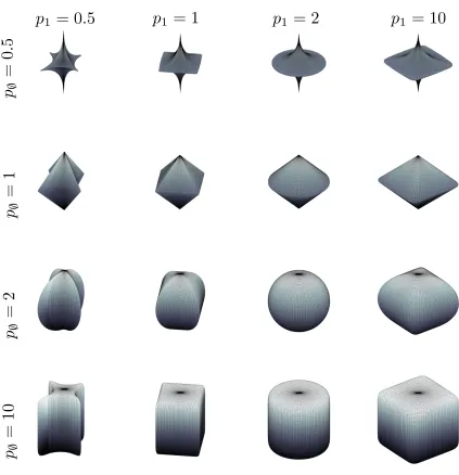
Lp-nested functions are much more flexible in creating different shapes of level sets than single
Lp-norms. Those level sets become the iso-density contours in the family of Lp-nested symmetric distributions. Figure 2 shows a variety of contours generated by the simplest non-trivial Lp-nested function shown in Equation (1). The shapes show the unit spheres for all possible combinations of p/0,p1∈ {0.5,1,2,10}. On the diagonal, p/0and p1are equal and therefore constitute Lp-norms. The corresponding distributions are members of the Lp-spherically symmetric class.
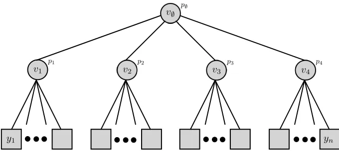
To make general statements about general Lp-nested functions, we introduce a notation that is suitable for the tree structure of Lp-nested functions. As we will heavily use that notation in the remainder of the paper, we would like to emphasize the importance of the following paragraphs. We will illustrate the notation with an example below. Additionally, Figure 1 and Table 1 can be used for reference.
We use multi-indices to denote the different nodes of the tree corresponding to an Lp-nested function f . The function f = f/0 itself computes the value v/0 at the root node (see Figure 1). Those values are denoted by variables v. The functions corresponding to its children are denoted by f1, ...,fℓ/0, that is, f(·) = f/0(·) =k(f1(·), ...,fℓ/0(·))kp/0. We always use the letter “ℓ” indexed by
(a) Equation (1) as tree. (b) Equation (1) as tree in multi-index notation.
Figure 1: Equation (1) visualized as a tree with two different naming conventions. Figure (a) shows the tree where the nodes are labeled with the coefficients of xxx∈Rn. Figure (b) shows the same tree in multi-index notation where the multi-index of a node describes the path from the root node to that node in the tree. The leaves v1,v2,1and v2,2still correspond to
x1,x2and x3, respectively, but have been renamed to the multi-index notation used in this article.
f(·) =f/0(·) Lp-nested function
I=i1, ...,im Multi-index denoting a node in the tree: The single indices describe the path from the root node to the respective node I.
xxxI All entries in xxx that correspond to the leaves in the subtree under the node I
xxxIb All entries in xxx that are not leaves in the subtree under the node I
fI(·) Lp-nested function corresponding to the subtree under the node I
v/0 Function value at the root node
vI Function value at an arbitrary node with multi-index I ℓI The number of direct children of a node I
nI The number of leaves in the subtree under the node I
vvvI,1:ℓI Vector with the function values at the direct children of a node I
Table 1: Summary of the notation used for Lp-nested functions in this article.
the children of the ith child of the root node are denoted by f
i,1, ...,fi,ℓi and so on. In this manner,
an index is added for denoting the children of a particular node in the tree and each multi-index denotes the path to the respective node in the tree. For the sake of compact notation, we use upper case letters to denote a single multi-index I=i1, ...,iℓ. The range of the single indices and the length
of the multi-index should be clear from the context. A concatenation I,k of a multi-index I with
Figure 2: Variety of contours created by the Lp-nested function of Equation (1) for all combinations of p/0,p1∈ {0.5,1,2,10}.
convention that I,/0=I. Those coefficients of the vector xxx that correspond to leaves of the subtree
under a node with the index I are denoted by xxxI. The complement of those coefficients, that is, the ones that are not in the subtree under the node I, are denoted by xxxbI. The number of leaves in a subtree under a node I is denoted by nI. If I denotes a leaf then nI=1.
The Lp-nested function associated with the subtree under a node I is denoted by
fI(xxxI) =||(fI,1(xxxI,1), ...,fI,ℓI(xxxI,ℓI))
Just like for the root node, we use the variable vIto denote the function value vI=fI(xxxI)of a subtree
I. A vector with the function values of the children of I is denoted with bold font vvvI,1:ℓI where the
colon indicates that we mean the vector of the function values of theℓI children of node I:
fI(xxxI) =||(fI,1(xxxI,1), ...,fI,ℓI(xxxI,ℓI))
⊤|| pI
=||(vI,1, ...,vI,ℓI)
⊤||
pI=||vvvI,1:ℓI||pI.
Note that we can assign an arbitrary p to leaf nodes since ps for single variables always cancel. For that reason we can choose an arbitrary p for convenience and fix its value to p=1. Figure 1(b) shows the multi-index notation for our example of Equation (1).
To illustrate the notation: Let I =i1, ...,id be the multi-index of a node in the tree. i1, ...,id describes the path to that node, that is, the respective node is the ithd child of the ithd−1 child of the ithd−2 child of the ... of the ith1 child of the root node. Assume that the leaves in the subtree below the node I cover the vector entries x2, ...,x10. Then xxxI= (x2, ...,x10), xxxbI = (x1,x11,x12, ...), and nI =9. Assume that node I has ℓI =2 children. Those would be denoted by I,1 and I,2. The function realized by node I would be denoted by fI and only acts on xxxI. The value of the function would be fI(xxxI) =vI and the vector containing the values of the children of I would be
vvvI,1:2= (vI,1,vI,2)⊤= (fI,1(xxxI,1),fI,2(xxxI,2))⊤.
We now introduce a coordinate representation specially tailored to Lp-nested symmetrically distributed variables: One of the most important consequences of the positive homogeneity of f is that it can be used to “normalize” vectors and, by that property, create a polar like coordinate representation of a vector xxx. Such polar-like coordinates generalize the coordinate representation for Lp-norms by Gupta and Song (1997).
Definition 1 (Polar-like Coordinates) We define the following polar-like coordinates for a vector
xxx∈Rn:
ui=
xi
f(xxx) for i=1, ...,n−1,
r=f(xxx).
The inverse coordinate transformation is given by
xi=ruifor i=1, ...,n−1,
xn=r∆nun
where∆n=sgn xnand un= f|x(nxxx|).
Note that un is not part of the coordinate representation since normalization with 1/f(xxx) de-creases the degrees of freedom uuu by one, that is, un can always be computed from all other ui by solving f(uuu) = f(xxx/f(xxx)) =1 for un. We use the term un only for notational simplicity. With a slight abuse of notation, we will use uuu to denote the normalized vector xxx/f(xxx)or only its first n−1 components. The exact meaning should always be clear from the context.
transformation does not depend on the value of∆n and can be computed analytically. The deter-minant is essential for deriving the uniform distribution on the unit Lp-nested sphereLf, that is, the 1-level set of f . Apart from that, it can be used to compute the radial distribution for a given
Lp-nested symmetric distribution. We start by stating the general form of the determinant in terms of the partial derivatives ∂un
∂uk, ukand r. Afterwards we demonstrate that those partial derivatives have
a special form and that most of them cancel in Laplace’s expansion of the determinant.
Lemma 2 (Determinant of the Jacobian) Let r and uuu be defined as in Definition 1. The general form of the determinant of the Jacobian
J
=∂xi∂yj
i j of the inverse coordinate transformation for
y1=r and yi=ui−1for i=2, ...,n, is given by
|det
J
|=rn−1 −n−1
∑
k=1
∂un
∂uk
·uk+un
!
. (2)
Proof The proof can be found in the Appendix A.
The problematic parts in Equation (2) are the terms ∂un
∂uk, which obviously involve extensive usage
of the chain rule. Fortunately, most of them cancel when inserting them back into Equation (2), leaving a comparably simple formula. The remaining part of this section is devoted to computing those terms and demonstrating how they vanish in the formula for the determinant. Before we state the general case we would like to demonstrate the basic mechanism through a simple example. We urge the reader to follow this example as it illustrates all important ideas about the coordinate transformation and its Jacobian.
Example 1 Consider an Lp-nested function very similar to our introductory example of Equation
(1):
f(xxx) =(|x1|p1+|x2|p1)
p/0
p1+|x3|p/0
1
p/0
.
Setting uuu= xxx
f(xxx)and solving for u3yields
f(uuu) =1⇔ u3=
1−(|u1|p1+|u2|p1)
p/0 p1
1
p/0
. (3)
We would like to emphasize again, that u3is actually not part of the coordinate representation and
only used for notational simplicity. By construction, u3is always positive. This is no restriction since
Lemma 2 shows that the determinant of the Jacobian does not depend on its sign. However, when computing the volume and the surface area of the Lp-nested unit sphere, it will become important
since it introduces a factor of 2 to account for the fact that u3 (or unin general) can in principle
also attain negative values. Now, consider
G2(uuub2) =g2(uuub2)
1−p/0 =1−(|u
1|p1+|u2|p1)
p/0 p1
1−p/0 p/0
,
F1(uuu1) =f1(uuu1)p/0−p1= (|u1|p1+|u2|p1)
where the subindices of uuu, f,g,G and F have to be read as multi-indices. The function gIcomputes
the value of the node I from all other leaves that are not part of the subtree under I by fixing the value of the root node to one.
G2(uuub2)and F1(uuu1)are terms that arise from applying the chain rule when computing the partial
derivatives ∂u3
∂uk. Taking those partial derivatives can be thought of as peeling off layer by layer
of Equation (3) via the chain rule. By doing so, we “move” on a path between u3 and uk. Each
application of the chain rule corresponds to one step up or down in the tree. First, we move upwards in the tree, starting from u3. This produces the G-terms. In this example, there is only one step
upwards, but in general, there can be several, depending on the depth of unin the tree. Each step
up will produce one G-term. At some point, we will move downwards in the tree to reach uk. This
will produce the F-terms. While there are as many G-terms as upward steps, there is one term less when moving downwards. Therefore, in this example, there is one term G2(uuub2)which originates
from using the chain rule upwards in the tree and one term F1(uuu1)from using it downwards. The
indices correspond to the multi-indices of the respective nodes. Computing the derivative yields
∂u3
∂uk
=−G2(uuub2)F1(uuu1)∆k|uk| p1−1.
By inserting the results in Equation (2) we obtain
1
r2|
J
|= 2∑
k=1
G2(uuub2)F1(uuu1)|uk| p1+u
3
=G2(uuub2) F1(uuu1) 2
∑
k=1
|uk|p1+1−F1(uuu1)F1(uuu1)−1(|u1|p1+|u2|p1)
p/0 p1
!
=G2(uuub2) F1(uuu1) 2
∑
k=1
|uk|p1+1−F1(uuu1) 2
∑
k=1
|uk|p1
!
=G2(uuub2).
The example suggests that the terms from using the chain rule downwards in the tree cancel while the terms from using the chain rule upwards remain. The following proposition states that this is true in general.
Proposition 3 (Determinant of the Jacobian) Let
L
be the set of multi-indices of the path from the leaf un to the root node (excluding the root node) and let the terms GI,ℓI(uuuIc,ℓI)recursively bedefined as
GI,ℓI(uuuIc,ℓI) =gI,ℓI(uuuIc,ℓI)
pI,ℓI−pI = gI(uuu b
I) pI−
ℓ−1
∑
j=1
fI,j(uuuI,j)pI
!pI,ℓI−pI pI
where each of the functions gI,ℓI computes the value of theℓ
th child of a node I as a function of its
neighbors(I,1),...,(I, ℓI−1)and its parent I while fixing the value of the root node to one. This
is equivalent to computing the value of the node I from all coefficients uuubI that are not leaves in the subtree under I. Then, the determinant of the Jacobian for an Lp-nested function is given by
|det
J
|=rn−1∏
L∈L
Proof The proof can be found in the Appendix A.
Let us illustrate the determinant with two examples:
Example 2 Consider a normal Lp-norm
f(xxx) =
n
∑
i=1
|xi|p
!1
p
which is obviously also an Lp-nested function. Resolving the equation for the last coordinate of
the normalized vector uuu yields gn(uuubn) =un= 1−∑n−1i=1|ui|p
1
p. Thus, the term G
n(uuubn)is given by 1−∑n−1i=1|ui|p
1−p
p which yields a determinant of|det
J
|=rn−1 1−∑n−1i=1|ui|p
1−p
p . This is exactly
the one derived by Gupta and Song (1997).
Example 3 Consider the introductory example
f(xxx) =|x1|p/0+ (|x2|p1+|x3|p1)
p/0 p1
1
p/0
.
Normalizing and resolving for the last coordinate yields
u3=
(1− |u1|p/0)
p1 p/0 − |u
2|p1
1
p1
and the terms G2(uuub2)and G2,2(uuu2c,2)of the determinant|det
J
|=r 2G2(uuub2)G2,2(uuu2c,2)are given by
G2(uuub2) = (1− |u1|
p/0)p1p−/0p/0 ,
G2,2(uuu2c,2) =
(1− |u1|p/0)
p1 p/0 − |u
2|p1
1−p1
p1
.
Note the difference to Example 1 where x3 was at depth one in the tree while x3 is at depth two in
the current case. For that reason, the determinant of the Jacobian in Example 1 involved only one G-term while it has two G-terms here.
3. Lp-Nested Symmetric and Lp-Nested Uniform Distribution
In this section, we define the Lp-nested symmetric and the Lp-nested uniform distribution and derive their partition functions. In particular, we derive the surface area of an arbitrary Lp-nested unit sphereLf ={xxx∈Rn| f(xxx) =1} corresponding to an Lp-nested function f . By Equation (5) of Fernandez et al. (1995) everyν-spherical and hence any Lp-nested symmetric density has the form
ρ(xxx) = φ(f(xxx))
f(xxx)n−1
S
f(1), (4)
Proposition 4 (Volume and Surface of the Lp-nested Sphere) Let f be an Lp-nested function and
let
I
be the set of all multi-indices denoting the inner nodes of the tree structure associated with f . The volumeV
f(R)and the surfaceS
f(R)of the Lp-nested sphere with radius R are given byV
f(R) =Rn2n
n
∏
I∈I1
pℓI−1
I
ℓI−1
∏
k=1
B
"
∑k
i=1nI,k
pI
,nI,k+1
pI
#!
(5)
=R
n2n
n
∏
I∈I∏ℓI
k=1Γ
hn
I,k
pI
i
pℓI−1
I Γ
h
nI
pI
i , (6)
S
f(R) =Rn−12n∏
I∈I1
pℓI−1
I
ℓI−1
∏
k=1
B
"
∑k
i=1nI,k
pI
,nI,k+1
pI
#!
(7)
=Rn−12n
∏
I∈I
∏ℓI
k=1Γ
hn
I,k
pI
i
pℓI−1
I Γ
h
nI
pI
i (8)
where B[a,b] =ΓΓ[[aa]+Γ[bb]] denotes theβ-function.
Proof The proof can be found in the Appendix B.
Inserting the surface area in Equation 4, we obtain the general form of an Lp-nested symmetric distribution for any given radial densityφ.
Corollary 5 (Lp-nested Symmetric Distribution) Let f be an Lp-nested function andφa density
onR+. The corresponding Lp-nested symmetric distribution is given by
ρ(xxx) = φ(f(xxx))
f(xxx)n−1
S
f(1)= φ(f(xxx))
2nf(xxx)n−1
∏
I∈I
pℓI−1
I
ℓI−1
∏
k=1
B
"
∑k
i=1nI,k
pI
,nI,k+1
pI
#−1
. (9)
The results of Fernandez et al. (1995) imply that for anyν-spherically symmetric distribution, the radial part is independent of the directional part, that is, r is independent of uuu. The distribution
of uuu is entirely determined by the choice of ν, or by the Lp-nested function f in our case. The distribution of r is determined by the radial densityφ. Together, an Lp-nested symmetric distribution is determined by both, the Lp-nested function f and the choice ofφ. From Equation (9), we can see that its density function must be the inverse of the surface area ofLf times the radial density when transforming (4) into the coordinates of Definition 1 and separating r and uuu (the factor f(xxx)n−1=r cancels due to the determinant of the Jacobian). For that reason we call the distribution of uuu uniform on the Lp-sphereLf in analogy to Song and Gupta (1997). Next, we state its form in terms of the coordinates uuu.
Proposition 6 (Lp-nested Uniform Distribution) Let f be an Lp-nested function. Let
L
be thedistribution on the Lp-nested unit sphere, that is, the setLf ={xxx∈Rn|f(xxx) =1}is given by the
following density over u1, ...,un−1
ρ(u1, , ...,un−1) =∏L∈L
GL(uuubL) 2n−1
∏
I∈I
pℓI−1
I
ℓI−1
∏
k=1
B
"
∑k
i=1nI,k
pI
,nI,k+1
pI
#−1
.
Proof Since the Lp-nested sphere is a measurable and compact set, the density of the uniform dis-tribution is simply one over the surface area of the Lp-nested unit sphere. The surface
S
f(1)is given by Proposition 4. TransformingS1f(1)into the coordinates of Definition 1 introduces the determinant
of the Jacobian from Proposition 3 and an additional factor of 2 since the(u1, ...,un−1)∈Rn−1have to account for both half-shells of the Lp-nested unit sphere, that is, to account for the fact that un could have been be positive or negative. This yields the expression above.
Example 4 Let us again demonstrate the proposition at the special case where f is an Lp-norm
f(xxx) =||xxx||p= (∑ni=1|xi|p) 1
p. Using Proposition 4, the surface area is given by
S
||·||p =2n 1pℓ/0/0−1 ℓ/0−1
∏
k=1
B
∑k
i=1nk
p/0 ,
nk+1
p/0
=
2nΓnh1pi
pn−1Γhn p
i.
The factor Gn(uuubn)is given by 1−∑n−1i=1|ui|p
1−p
p (see the L
p-norm example before), which, after
including the factor 2, yields the uniform distribution on the Lp-sphere as defined in Song and Gupta
(1997)
p(uuu) =
pn−1Γ
h
n p
i
2n−1Γnh1 p
i 1−
n−1
∑
i=1
|ui|p
!1−p
p
.
Example 5 As a second illustrative example, we consider the uniform density on the Lp-nested
unit ball, that is, the set{xxx∈Rn|f(xxx)≤1}, and derive its radial distributionφ. The density of the uniform distribution on the unit Lp-nested ball does not depend on xxx and is given byρ(xxx) =1/
V
f(1).Transforming the density into the polar-like coordinates with the determinant from Proposition 3 yields
1
V
f(1)=nr
n−1∏
L∈LGL(uuubL) 2n−1
∏
I∈I
pℓI−1
I
ℓI−1
∏
k=1
B
"
∑k
i=1nI,k
pI
,nI,k+1
pI
#−1
.
After separating out the uniform distribution on the Lp-nested unit sphere, we obtain the radial
distribution
φ(r) =nrn−1for 0<r≤1
The radial distribution from the preceeding example is of great importance for our sampling scheme derived in Section 6. The idea behind it is the following: First, a sample from a “simple”
Lp-nested symmetric distribution is drawn. Since the radial and the uniform component on the Lp -nested unit sphere are statistically independent, we can get a sample from the uniform distribution on the Lp-nested unit sphere by simply normalizing the sample from the simple distribution. After-wards we can multiply it with a radius drawn from the radial distribution of the Lp-nested symmetric distribution that we actually want to sample from. The role of the simple distribution will be played by the uniform distribution within the Lp-nested unit ball. Sampling from it is basically done by applying the steps in Proposition 4’s proof backwards. We lay out the sampling scheme in more detail in Section 6.
4. Marginals
In this section we discuss two types of marginals: First, we demonstrate that, in contrast to Lp -spherically symmetric distributions, marginals of Lp-nested symmetric distributions are not nec-essarily Lp-nested symmetric again. The second type of marginals we discuss are obtained by collapsing all leaves of a subtree into the value of the subtree’s root node. For that case we derive an analytical expression and show that the values of the root node’s children follow a special kind of Dirichlet distribution.
Gupta and Song (1997) show that marginals of Lp-spherically symmetric distributions are again
Lp-spherically symmetric. This does not hold, however, for Lp-nested symmetric distributions. This can be shown by a simple counterexample. Consider the Lp-nested function
f(xxx) =(|x1|p1+|x2|p1)
p/0
p1+|x3|p/0
1
p/0
.
The uniform distribution inside the Lp-nested ball corresponding to f is given by
ρ(xxx) =
np1p/0Γ
h
2 p1
i
Γh3
p/0 i
23Γ2h1 p1
i
Γh2
p0
i
Γh1
p0
i.
The marginalρ(x1,x3)is given by
ρ(x1,x3) =
np1p/0Γ
h
2 p1
i
Γh3
p/0 i
23Γ2h1 p1
i
Γh2
p0
i
Γh1
p0
i(1− |x3|p/0)
p1 p/0 − |x
1|p1
1
p1
.
This marginal is not Lp-spherically symmetric. Since any Lp-nested symmetric distribution in two dimensions must be Lp-spherically symmetric, it cannot be Lp-nested symmetric as well. Figure 3 shows a scatter plot of the marginal distribution. Besides the fact that the marginals are not contained in the family of Lp-nested symmetric distributions, it is also hard to derive a general form for them. This is not surprising given that the general form of marginals for Lp-spherically symmetric distributions involves an integral that cannot be solved analytically in general and is therefore not very useful in practice (Gupta and Song, 1997). For that reason we cannot expect marginals of Lp-nested symmetric distributions to have a simple form.
a
b
c
d
Figure 3: Marginals of Lp-nested symmetric distributions are not necessarily Lp-nested symmetric: Figure (a) shows a scatter plot of the(x1,x2)-marginal of the counterexample in the text with p/0=2 and p1= 12. Figure (d) displays the corresponding Lp-nested sphere. (b-c) show the univariate marginals for the scatter plot. Since any two-dimensional Lp -nested symmetric distribution must be Lp-spherically symmetric, the marginals should be identical. This is clearly not the case. Thus, (a) is not Lp-nested symmetric.
the Lp-nested tree vertically, we call this type of marginals layer marginals. In the following, we present their general form.
From the form of a general Lp-nested function and the corresponding symmetric distribution, one might think that the layer marginals are Lp-nested symmetric again. However, this is not the case since the distribution over the Lp-nested unit sphere would deviate from the uniform distribution in most cases if the distribution of its children were Lp-spherically symmetric.
Proposition 7 Let f be an Lp-nested function. Suppose we integrate out complete subtrees from
the tree associated with f , that is, we transform subtrees into radial times uniform variables and integrate out the latter. Let
J
be the set of multi-indices of those nodes that have become new leaves, that is, whose subtrees have been removed, and let nJbe the number of leaves (in the original tree)in the subtree under the node J. Let xxxbJ ∈Rm denote those coefficients of xxx that are still part of that smaller tree and let vvvJ denote the vector of inner nodes that became new leaves. The joint
distribution of xxxbJ and vvvJ is given by
ρ(xxxJb,vvvJ) =
φ(f(xxxbJ,vvvJ))
Sf(f(xxxbJ,vvvJ))J∈
∏
JvnJ−1
J . (10)
Proof The proof can be found in the Appendix C.
Equation (10) has an interesting special case when considering the joint distribution of the root node’s children.
Corollary 8 The children of the root node vvv1:ℓ/0 = (v1, ...,vℓ/0)⊤follow the distribution
ρ(vvv1:ℓ/0) =
pℓ/0/0−1Γhpn
/0 i
f(v1, ...,vℓ/0)n−12m∏ℓk/0=1Γ
h
nk
p/0
iφ(f(v1, ...,vℓ/0))
ℓ/0
∏
i=1
vni−1
i
where m≤ℓ/0 is the number of leaves directly attached to the root node. In particular, vvv1:ℓ/0 can
be written as the product RU , where R is the Lp-nested radius and the single |Ui|p/0 are Dirichlet
distributed, that is,(|U1|p/0, ...,|Uℓ/0|p/0)∼Dir h
n1 p/0, ...,
nℓ/0
p/0 i
.
Proof The joint distribution is simply the application of Proposition (7). Note that f(v1, ...,vℓ/0) =
||vvv1:ℓ/0||p/0. Applying the pointwise transformation si=|ui|p/0 yields
(|U1|p/0, ...,|Uℓ/0−1|p/0)∼Dir
n1
p/0, ...,
nℓ/0 p/0
.
The Corollary shows that the values fI(xxxI)at inner nodes I, in particular the ones directly below the root node, deviate considerably from Lp-spherical symmetry. If they were Lp-spherically sym-metric, the|Ui|pshould follow a Dirichlet distribution with parametersαi= 1p as has been already shown by Song and Gupta (1997). The Corollary is a generalization of their result.
Proposition 9 Let xxx be Lp-nested symmetric distributed with independent marginals. Then xxx is
Lp-spherically symmetric distributed. In particular, xxx follows a p-generalized Normal distribution.
Proof The proof can be found in the Appendix D.
One immediate implication of Proposition 9 is that there is no factorial probability model corre-sponding to mixed norm regularizers which have the form∑ki=1kxxxIkk
q
pwhere the index sets Ikform a partition of the dimensions 1, ...,n (see, e.g., Zhao et al., 2008; Yuan and Lin, 2006; Kowalski
et al., 2008). Many machine learning algorithms are equivalent to minimizing the sum of a regu-larizer R(www)and a loss function L(www,xxx1, ...,xxxm) over the coefficient vector www. If the exp(−R(www)) and exp(−L(www,xxx1, ...,xxxm)) correspond to normalizeable density models, the minimizing solution of the objective function can be seen as the maximum a posteriori (MAP) estimate of the poste-rior p(www|xxx1, ...,xxxm)∝p(www)·p(xxx1, ...,xxxm|www) =exp(−R(www))·exp(−L(www,xxx1, ...,xxxm)). In that sense, the regularizer naturally corresponds to the prior and the loss function corresponds to the likeli-hood. Very often, regularizers are specified as a norm over the coefficient vector www which in turn
correspond to certain priors. For example, in Ridge regression (Hoerl, 1962) the coefficients are regularized viakwwwk2
2which corresponds to a factorial zero mean Gaussian prior on www. The L1-norm
kwwwk1in the LASSO estimator (Tibshirani, 1996), again, is equivalent to a factorial Laplacian prior on www. Like in these two examples, regularizers often correspond to a factorial prior.
Mixed norm regularizers naturally correspond to Lp-nested symmetric distributions. Proposition 9 shows that there is no factorial prior that corresponds to such a regularizer. In particular, it implies that the prior cannot be factorial between groups and coefficients at the same time. This means that those regularizers implicitly assume statistical dependencies between the coefficient variables. Interestingly, for q=1 and p=2 the intuition behind these regularizers is exactly that whole groups
Ikget switched on at once, but the groups are sparse. The Proposition shows that this might not only be due to sparseness but also due to statistical dependencies between the coefficients within one group. The Lp-nested symmetric distribution which implements independence between groups will be further discussed below as a generalization of the p-generalized Normal (see Section 8). Note that the marginals can be independent if the regularizer is of the form ∑ki=1kxxxIkk
p
p. However, in this case p=q and the Lp-nested function collapses to a simple Lp-norm which means that the regularizer is not mixed norm.
5. Maximum Likelihood Estimation of Lp-Nested Symmetric Distributions
In this section, we describe procedures for maximum likelihood fitting of Lp-nested symmetric dis-tributions on data. We provide a toolbox online for fitting Lp-spherically symmetric and Lp-nested symmetric distributions to data. The toolbox can be downloaded athttp://www.kyb.tuebingen. mpg.de/bethge/code/.
Depending on which parameters are to be estimated, the complexity of fitting an Lp-nested symmetric distribution varies. We start with the simplest case and later continue with more complex ones. Throughout this subsection, we assume that the model has the form p(xxx) =ρ(W xxx)· |detW|=
φ(W xxx)
f(W xxx)n−1S
f(1)· |detW|where W ∈R
n×n is a complete whitening matrix. This means that given any whitening matrix W0, the freedom in fitting W is to estimate an orthonormal matrix Q∈SO(n)
distributions can be endowed with 2nd-order correlations via W . In the following, we ignore the determinant of W since data points can always be rescaled such that detW=1.
The simplest case is to fit the parameters of the radial distribution when the tree structure, the values of the pI, and W are fixed. Due to the special form of Lp-nested symmetric distributions (4), it then suffices to carry out maximum likelihood estimation on the radial component only, which renders maximum likelihood estimation efficient and robust. This is because the only remaining parameters are the parametersϑϑϑof the radial distribution and, therefore,
argmaxϑϑϑlogρ(W xxx|ϑϑϑ) =argmaxϑϑϑ(−log
S
f(f(W xxx)) +logφ(f(W xxx)|ϑϑϑ))=argmaxϑϑϑlogφ(f(W xxx)|ϑϑϑ).
In a slightly more complex case, when only the tree structure and W are fixed, the values of the
pI,I ∈
I
andϑϑϑcan be jointly estimated via gradient ascent on the log-likelihood. The gradient for a single data point xxx with respect to the vector ppp that holds all pI for all I∈I
is given by∇ppplogρ(W xxx) =
d
drlogφ(f(W xxx))·∇pppf(W xxx)−
(n−1)
f(W xxx)∇pppf(W xxx)−∇ppplogSf(1).
For i.i.d. data points xxxithe joint gradient is given by the sum over the gradients for the single data points. Each of them involves the gradient of f as well as the gradient of the log-surface area ofLf with respect to ppp, which can be computed via the recursive equations
∂
∂pJ
vI=
0 if I is not a prefix of J
v1−pI
I v pI−1
I,k ·∂∂pJvI,k if I is a prefix of J
vJ
pJ
v−pJ
J ∑
ℓJ
k=1v pJ
J,k·log vJ,k−log vJ
if J=I
and
∂
∂pJ
log
S
f(1) =− ℓJ−1pJ
+
ℓJ−1
∑
k=1
Ψ "
∑k+1
i=1nJ,k
pJ
#
∑k+1
i=1nJ,k
p2J −
ℓJ−1
∑
k=1
Ψ "
∑k
i=1nJ,k
pJ
#
∑k
i=1nJ,k
p2J − ℓJ−1
∑
k=1
ΨnJ,k+1
pJ
nJ,k+1
p2J ,
whereΨ[t] = d
dtlogΓ[t]denotes the digamma function. When performing the gradient ascent, one needs to set 000 as a lower bound for ppp. Note that, in general, this optimization might be a highly
non-convex problem.
On the next level of complexity, only the tree structure is fixed, and W can be estimated along with the other parameters by joint optimization of the log-likelihood with respect to ppp,ϑϑϑand W . Certainly, this optimization problem is also not convex in general. Usually, it is numerically more robust to whiten the data first with some whitening matrix W0and perform a gradient ascent on the special orthogonal group SO(n) with respect to Q for optimizing W =QW0. Given the gradient
∇Wlogρ(W xxx)of the log-likelihood, the optimization can be carried out by performing line searches along geodesics as proposed by Edelman et al. (1999) (see also Absil et al. (2007)) or by projecting
The general form of the gradient to be used in such an optimization scheme can be defined as
∇Wlogρ(W xxx)
=∇W(−(n−1)·log f(W xxx) +logφ(f(W xxx)))
=−(n−1)
f(W xxx)·∇yyyf(W xxx)·xxx
⊤+d logφ(r)
dr (f(W xxx))·∇yyyf(W xxx)·xxx
⊤,
where the derivatives of f with respect to yyy are defined by recursive equations
∂
∂yi
vI=
0 if i6∈I
sgn yi if vI,k=|yi|
v1−pI
I ·v pI−1
I,k ·∂∂yivI,k for i∈I,k.
Note, that f might not be differentiable at yyy=0. However, we can always define a sub-derivative at zero, which is zero for pI6=1 and[−1,1]for pI=1. Again, the gradient for i.i.d. data points xxxiis given by the sum over the single gradients.
Finally, the question arises whether it is possible to estimate the tree structure from data as well. A simple heuristic would be to start with a very large tree, for example, a full binary tree, and to prune out inner nodes for which the parents and the children have sufficiently similar values for their
pI. The intuition behind this is that if they were exactly equal, they would cancel in the Lp-nested function. This heuristic is certainly sub-optimal. Firstly, the optimization will be time consuming since there can be about as many pI as there are leaves in the Lp-nested tree (a full binary tree on n dimensions will have n−1 inner nodes) and due to the repeated optimization after the pruning steps. Secondly, the heuristic does not cover all possible trees on n leaves. For example, if two leaves are separated by the root node in the original full binary tree, there is no way to prune out inner nodes such that the path between those two nodes will not contain the root node anymore.
The computational complexity for the estimation of all other parameters despite the tree struc-ture is difficult to assess in general because they depend, for example, on the particular radial dis-tribution used. While the maximum likelihood estimation of a simple log-Normal disdis-tribution only involves the computation of a mean and a variance which are in
O
(m)for m data points, a mixture of log-Normal distributions already requires an EM algorithm which is computationally more expen-sive. Additionally, the time it takes to optimize the likelihood depends on the starting point as well as the convergence rate, and we neither have results about the convergence rate nor is it possible to make problem independent statements about a good initialization of the parameters. For this reason we state only the computational complexity of single steps involved in the optimization.costs per step increase to
O
(n3+n2m) since m data points have to be multiplied with W at each iteration (requiringO
(n2m)steps), and the line search involves projecting Q back onto SO(n)which requires an inverse matrix square root or a similar computation inO
(n3).For comparison, each step of fast ICA (Hyv¨arinen and O., 1997) for a complete demixing matrix takes
O
(n2m)when using hierarchical orthogonalization andO
(n2m+n3)for symmetric orthogo-nalization. The same applies to fitting an ISA model (Hyv¨arinen and Hoyer, 2000; Hyv¨arinen and K¨oster, 2006, 2007). A Gaussian Scale Mixture (GSM) model does not need to estimate an-other orthogonal rotation Q because it belongs to the class of spherically symmetric distributions and is, therefore, invariant under transformations from SO(n)(Wainwright and Simoncelli, 2000). Therefore, fitting a GSM corresponds to estimating the parameters of the scale distribution which isO
(nm)in the best case but might be costlier depending on the choice of the scale distribution.6. Sampling from Lp-Nested Symmetric Distributions
In this section, we derive a sampling scheme for arbitrary Lp-nested symmetric distributions which can for example be used for solving integrals when using Lp-nested symmetric distributions for Bayesian learning. Exact sampling from an arbitrary Lp-nested symmetric distribution is in fact straightforward due to the following observation: Since the radial and the uniform component are in-dependent, normalizing a sample from any Lp-nested symmetric distribution to f -length one yields samples from the uniform distribution on the Lp-nested unit sphere. By multiplying those uni-form samples with new samples from another radial distribution, one obtains samples from another
Lp-nested symmetric distribution. Therefore, for each Lp-nested function f , a single Lp-nested sym-metric distribution which can be easily sampled from is enough. Sampling from all other Lp-nested symmetric distributions with respect to f is then straightforward due to the method we just de-scribed. Gupta and Song (1997) sample from the p-generalized Normal distribution since it has in-dependent marginals which makes sampling straightforward. Due to Proposition 9, no such factorial
Lp-nested symmetric distribution exists. Therefore, a sampling scheme like that for Lp-spherically symmetric distributions is not applicable. Instead we choose to sample from the uniform distribu-tion inside the Lp-nested unit ball for which we already computed the radial distribudistribu-tion in Example 5. The distribution has the formρ(xxx) = V1
f(1). In order to sample from that distribution, we will first
only consider the uniform distribution in the positive quadrant of the unit Lp-nested ball which has the formρ(xxx) = 2n
Vf(1). Samples from the uniform distributions inside the whole ball can be obtained
by multiplying each coordinate of a sample with independent samples from the uniform distribution over{−1,1}.
The idea of the sampling scheme for the uniform distribution inside the Lp-nested unit ball is based on the computation of the volume of the Lp-nested unit ball in Proposition 4. The basic mechanism underlying the sampling scheme below is to apply the steps of the proof backwards, which is based on the following idea: The volume of the Lp-unit ball can be computed by computing its volume on the positive quadrant only and multiplying the result with 2nafterwards. The key is now to not transform the whole integral into radial and uniform coordinates at once, but successively upwards in the tree. We will demonstrate this through a brief example which also should make the sampling scheme below more intuitive. Consider the Lp-nested function
f(xxx) =|x1|p/0+ (|x2|p1+|x3|p1)
p/0 p1
1
p/0
To solve the integral Z
{xxx: f(xxx)≤1 & xxx∈Rn
+}
dxxx,
we first transform x2and x3into radial and uniform coordinates only. According to Proposition 3 the determinant of the mapping(x2,x3)7→(v1,u˜) = (kxxx2:3kp1,xxx2:3/kxxx2:3kp1)is given by v1(1−u˜
p1) 1−p1
p1 .
Therefore the integral transforms into Z
{xxx: f(xxx)≤1 & xxx∈Rn
+}
dxxx=
Z
{v1,x1: f(x1,v1)≤1 & x1,v1∈R+}
Z Z
v1(1−u˜p1) 1−p1
p1 dx1dv1d ˜u.
Now we can separate the integrals over x1and v1, and the integral over ˜u, since the boundary of the
outer integral does only depend on v1and not on ˜u:
Z
{xxx: f(xxx)≤1 & xxx∈Rn+}
dxxx=
Z
(1−u˜p1) 1−p1
p1 d ˜u·
Z
{v1,x1: f(x1,v1)≤1 & x1,v1∈R+}
Z
v1dx1dv1.
The value of the first integral is known explicitly since the integrand equals the uniform distribution on thek · kp1-unit sphere. Therefore, the value of the integral must be its normalization constant which we can get using Proposition 4:
Z
(1−u˜p1) 1−p1
p1 d ˜u=
Γh1
p1
i2
·p1
Γh2
p1
i .
An alternative way to arrive at this result is to use the transformation s=u˜p1 and to notice that the integrand is a Dirichlet distribution with parametersαi= p1
1. The normalization constant of the Dirichlet distribution and the constants from the determinant of the Jacobian of the transformation yield the same result.
To compute the remaining integral, the same method can be applied again yielding the volume of the Lp-nested unit ball. The important part for the sampling scheme, however, is not the volume itself but the fact that the intermediate results in this integration process equal certain distributions. As shown in Example 5 the radial distribution of the uniform distribution on the unit ball isβ[n,1], and as just indicated by the example above, the intermediate results can be seen as transformed variables from a Dirichlet distribution. This fact holds true even for more complex Lp-nested unit balls although the parameters of the Dirichlet distribution can be slightly different. Reversing the steps leads us to the following sampling scheme. First, we sample from theβ-distribution which gives us the radius v/0on the root node. Then we sample from the appropriate Dirichlet distribution and exponentiate the samples by p1/0 which transforms them into the analogs of the variable u from above. Scaling the result with the sample v/0 yields the values of the root node’s children, that is, the analogs of x1 and v1. Those are the new radii for the levels below them where we simply repeat this procedure with the appropriate Dirichlet distributions and exponents. The single steps are summarized in Algorithm 1.
The computational complexity of the sampling scheme is
O
(n). Since the sampling procedure is like expanding the tree node by node starting with the root, the number of inner nodes and leaves is the total number of samples that have to be drawn from Dirichlet distributions. Every node in anAlgorithm 1 Exact sampling algorithm for Lp-nested symmetric distributions
Input: The radial distributionφof an Lp-nested symmetric distributionρfor the Lp-nested function
f .
Output: Sample xxx fromρ. Algorithm
1. Sample v/0from a beta distributionβ[n,1].
2. For each inner node I of the tree associated with f , sample the auxiliary variable sssI from a Dirichlet distribution Dir
hn
I,1 pI , ...,
nI,ℓI
pI
i
where nI,k are the number of leaves in the subtree under node I,k. Obtain coordinates on the Lp-nested sphere within the positive orthant by
sssI7→sss 1
pI
I =uu˜uI(the exponentiation is taken component-wise).
3. Transform these samples to Cartesian coordinates by vI·uu˜uI=vvvI,1:ℓI for each inner node,
start-ing from the root node and descendstart-ing to lower layers. The components of vvvI,1:ℓI constitute
the radii for the layer direct below them. If I=/0, the radius had been sampled in step 1.
4. Once the two previous steps have been repeated until no inner node is left, we have a sample
xxx from the uniform distribution in the positive quadrant. Normalize xxx to get a uniform sample
from the sphere uuu= xxx f(xxx).
5. Sample a new radius ˜v/0 from the radial distribution of the target radial distribution φand obtain the sample via ˜xxx=v˜/0·uuu.
6. Multiply each entry xi of ˜xxx by an independent sample zi from the uniform distribution over
{−1,1}.
7. Robust Bayesian Inference of the Location
For Lp-spherically symmetric distributions with a location and a scale parameter
p(xxx|µµµ,τ) =τnρ(kτ(xxx−µµµ)kp),
Osiewalski and Steel (1993) derived the posterior in closed form using a prior p(µµµ,τ) =p(µ)·c·τ−1, and showed that p(xxx,µµµ)does not depend on the radial distributionφ, that is, the particular type of
Lp-spherically symmetric distributions used for a fixed p. The prior onτcorresponds to an improper Jeffrey’s prior which is used to represent lack of prior knowledge on the scale. The main implication of their result is that Bayesian inference of the location µµµ under that prior on the scale does not
depend on the particular type of Lp-spherically symmetric distribution used for inference. This means that under the assumption of an Lp-spherically symmetric distributed variable, for a fixed p, one has to know the exact form of the distribution in order to compute the location parameter.
Proposition 10 For fixed values p/0,p1, ...and two independent priors p(µµµ,τ) =p(µµµ)·cτ−1 of the
location µ and the scaleτwhere the prior onτis an improper Jeffrey’s prior, the joint distribution p(xxx,µµµ)is given by
p(xxx,µµµ) = f(xxx−µµµ)−n·c·1 Z·p(µµµ),
where Z denotes the normalization constant of the Lp-nested uniform distribution.
Proof Given any Lp-nested symmetric distributionρ(f(xxx)), the transformation into the polar-like coordinates yields the following relation
1=
Z
ρ(f(xxx))dxxx=
Z Z
∏
L∈L
GL(uuubL)r
n−1ρ(r)drduuu=Z
∏
L∈L
GL(uuuLb)duuu·
Z
rn−1ρ(r)dr.
Since∏L∈LGL(uuubL)is the unnormalized uniform distribution on the Lp-nested unit sphere, the inte-gral must equal the normalization constant which we denote with Z for brevity (see Proposition 6 for an explicit expression). This implies thatρhas to fulfill
1
Z =
Z
rn−1ρ(r)dr.
Writing down the joint distribution of xxx,µµµ andτ, and using the substitution s=τf(xxx−µµµ)we obtain
p(xxx,µµµ) =
Z
τnρ(f(τ(xxx−µµµ)))·cτ−1·p(µµµ)dτ
=
Z
sn−1ρ(s)·c·p(µµµ)f(xxx−µµµ)−nds
= f(xxx−µµµ)−n·c·1 Z·p(µµµ).
Note that this result could easily be extended toν-spherical distributions. However, in this case the normalization constant Z cannot be computed for most cases and, therefore, the posterior would not be known explicitly.
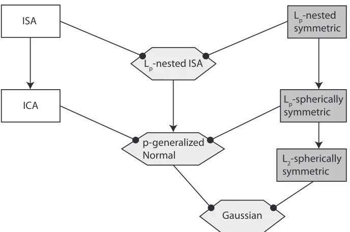
8. Relations to ICA, ISA and Over-Complete Linear Models
In this section, we explain the relations among Lp-spherically symmetric, Lp-nested symmetric, ICA and ISA models. For a general overview see Figure 4.
The density model underlying ICA models the joint distribution of the signal xxx as a linear superposition of statistically independent hidden sources Ayyy=xxx or yyy =W xxx. If the marginals
of the hidden sources belong to the exponential power family, we obtain the p-generalized Nor-mal which is a subset of the Lp-spherically symmetric class. The p-generalized Normal distri-bution p(yyy)∝exp(−τkyyykpp) is a density model that is often used in ICA algorithms for kurtotic natural signals like images and sound by optimizing a demixing matrix W w.r.t. to the model