CURVE is the Institutional Repository for Coventry University
A Comparative Study of the
Effectiveness of Adaptive Filter
Algorithms, Spectral Kurtosis and
Linear Prediction in Detection of a
Naturally Degraded Bearing in a
Gearbox
Elasha, F. , Ruiz-Carcel, C. , Mba, D. and Chandra, P.
Author post-print (accepted) deposited in CURVE January 2016Original citation & hyperlink:
Elasha, F. , Ruiz-Carcel, C. , Mba, D. and Chandra, P. (2014) A Comparative Study of the Effectiveness of Adaptive Filter Algorithms, Spectral Kurtosis and Linear Prediction in Detection of a Naturally Degraded Bearing in a Gearbox. Journal of Failure Analysis and Prevention , volume 14 (5): 623-636
http://dx.doi.org/10.1007/s11668-014-9857-8
ISSN 1547-7029 ESSN 1864-1245
DOI 10.1007/s11668-014-9857-8
Copyright © and Moral Rights are retained by the author(s) and/ or other copyright owners. A copy can be downloaded for personal non-commercial research or study, without prior permission or charge. This item cannot be reproduced or quoted extensively from without first obtaining permission in writing from the copyright holder(s). The content must not be changed in any way or sold commercially in any format or medium without the formal permission of the copyright holders.
This document is the author’s post-print version, incorporating any revisions agreed during the peer-review process. Some differences between the published version and this version may remain and you are advised to consult the published version if you wish to cite from it.
1
A comparative study of the effectiveness of adaptive filter algorithms, spectral kurtosis and linear prediction in detection of a naturally
degraded bearing in a gearbox.
F.Elasha1*, C.Ruiz-Carcel2, D. Mba2, P. Chandra3
1 School of Mechanical, Aerospace and automative Engineering, Coventry University (UK) 2
School of Engineering, Cranfield University (UK)
3
Moog Aircraft Group, Wolverhampton
Abstract
Diagnosing bearing faults at the earliest stages is critical in avoiding future catastrophic failures. Many techniques have been developed and applied in diagnosing bearings faults, however, these traditional diagnostic techniques are not always successful when the bearing fault occurs in gearboxes where the vibration response is complex; under such circumstances it may be necessary to separate the bearing signal from the complex signal.In this paper, an adaptive filter has been applied for the purpose of bearing signal separation. Four algorithms were compared to assess their effectiveness in diagnosing a bearing defect in a gearbox; Least Mean Square (LMS), Linear Prediction, Spectral Kurtosis (SK) and Fast Block LMS (FBLMS). These algorithms were applied to decompose the measured vibration signal into deterministic and random parts with the latter containing the bearing signal. Keywords:
Vibration, Adaptive filter, Signal separation, Bearing Diagnostics, Gearbox ______________
* corresponding author: Mechanical, Aerospace and automative Engineering, Coventry University, Coventry, UK
2
These techniques were applied to identify a bearing fault in a gearbox employed for an aircraft control system for which endurance tests were performed. The results show that the LMS algorithm is capable of detecting the bearing fault earlier in comparison to the other algorithms.
1
Introduction
Monitoring of machine vibration for early fault detection is widely applied [1 - 4]. The vibration signals from machines contain multiple sources which can be corrupted by noise from the transmission path. The diagnosis of bearing faults in gearboxes is not without its challenges [5-7], therefore methods of enhancing the signal to noise ratio (SNR) are required [8, 9]. This is particularly the case in gearboxes where the gear mesh contribution to the overall vibration is of such significance as to mask bearing fault frequencies [10-12]. In practice, envelope analysis has been used to extract the bearing fault vibration signature in gearboxes [13] though in some cases envelope analysis has failed to reduce the gear mesh contribution to the total vibration signal. In such instances a narrow band-pass filter at high frequency has been applied to separate the high frequency component excited by bearing impacts [14].
Early attempts utilize time domain averaging to separate the gear components from the measured vibration signal; in this case a delayed version of the signal is added to the vibration signal and this results in reinforcing some frequencies and cancelling others. However the signal to noise ratio (SNR) enhancement in this technique is not always sufficient to aid detection of bearing faults [15]. Time Synchronous Average (TSA) techniques are also applied to separate the bearing components from the gearboxes. With this technique the effect of the speed variation is removed by resampling the signal in the angular domain [8].
3
The process of resampling the signal is difficult and not commonly applied if the purpose is to separate the bearing signal [16].
Recently, signal separation techniques have been applied in the diagnosis of bearing faults within gearboxes. The separation is based on decomposing the signal into deterministic and random components. The deterministic part represents the gear component and the random part represents the bearings component of vibration. The bearing contribution to the signal is expected to be random due to slip effects [17].
More recently, the use of adaptive filters has been applied to monitor bearings [18-20]. This concept is based on the Wold Theorem, in which the signal can be decomposed into deterministic and non-deterministic parts [21]. It has been applied to signal processing in telecommunication [22] and ECG signal processing [23]. The separation is based on the fact that the deterministic part has a longer correlation than the random part and therefore the autocorrelation is used to distinguish the deterministic part from the random part. However a reference signal is required to perform the separation. The application of this theory in condition monitoring was established by Chaturvedi et al [24] where the Adaptive Noise Cancellation (ANC) algorithm was applied to separate bearing vibrations corrupted by engine noise with the bearing vibration signature used as a reference signal for the separation process. However, for practical diagnostics, the reference signal is not always readily available. As an alternative a delayed version of the signal has been proposed as a reference signal and this method is known as self-adaptive noise cancellation (SANC) [25] which is based on delaying the signal until the noise correlation is diminished and only the deterministic part is correlated [26].
4
Many recursive algorithms have been developed for application of the adaptive filter[20, 27]. Each algorithm offers its own features and therefore the algorithm to be employed should be selected carefully depending on the signal under consideration. Selection of the appropriate algorithm is determined by many factors including: convergence, computation cost, type of signal (stationary or non-stationary), and accuracy [28].
As noted earlier, in real applications background noise often masks the signal of interest and as a result the Kurtosis is unable to capture the peakness of the fault signal, giving usually low Kurtosis values. Therefore, in applications with strong background noise, the Kurtosis as a global indicator is not useful, though it gives better results when it is applied locally in different frequency bands [29]. The Spectral Kurtosis (SK) was first introduced by Dwyer in [30] as a statistical tool which can locate non-Gaussian components in the frequency domain of a signal. This method is able to indicate the presence of transients in the signal and show their locations in the frequency domain. It has demonstrated to be effective even in the presence of strong additive noise [29].
Four algorithms were compared to assess their effectiveness in diagnosing a bearing defect in a gearbox; Least Mean Square (LMS), Linear Prediction, Spectral Kurtosis (SK) and Fast Block LMS (FBLMS). These algorithms were applied to decompose the measured vibration signal into deterministic and random parts with the latter containing the bearing signal. In addition the result of the adaptive filter algorithms will be compared to the result of linear prediction and spectral kurtosis. This investigation assesses the merits of these techniques in identifying a natural degraded bearing under conditions of relatively large background noise. The gearbox considered in this study is part of a transmission system of an aircraft control system which suffered premature
5
bearing failure at an early stage of testing; therefore, these algorithms will be applied to examine their ability to identify the failure at the onset of degradation.
2
Theoretical background:
2.1 Adaptive filter
An adaptive filter is used to model the relationship between two signals in an iterative manner; the adaption refers to the method used to iterate the filter coefficient. The adaptive filter solution is not unique however the best solution is that which is closest to the desirable response signal [31]. FIR filters are more commonly used as adaptive filters in comparison of IRR filters [32].
The adaptive filter concept is based on Wold theorem which proposes that the vibration signal can be decomposed into two parts, deterministic 𝑃(𝑛) and random 𝑟 (𝑛). This decomposition process can be represented by the following formula [27] :
𝑥(𝑛) = 𝑃(𝑛) + 𝑟 (𝑛) (1)
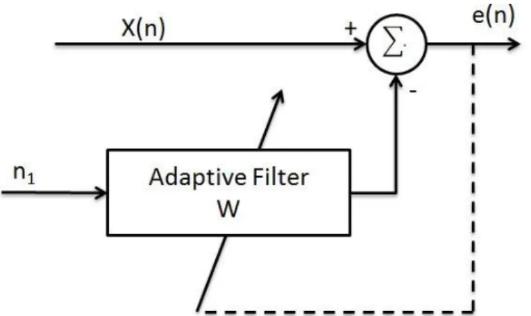
In the equation above the deterministic part can be predicted based on the history of the signal and the minimal prediction error, however the random part component cannot be predicted. The process of separation begins by applying adaptive noise cancellation (ANC), the fundamentals of this method have been detailed, and the general layout of the ANC algorithm is shown in Figure 1 [27, 33].
6
Figure 1 ANC algorithm
In application of the self-adaptive Least Mean Square (LMS) algorithm the reference signal in the application of ANC algorithm is replaced by a delayed version of the input signal. In this algorithm the signal is filtered using a wiener filter, the coefficients of which should be updated for each step, consequently feedback from the filter output is required to estimate the filter coefficients. This process is repeated for each filter step until the prediction error reaches the minimum value. The adaptive filter is a special case of FIR filter expressed by the following relation:
𝑌𝑖 = ∑ ℎ𝑖 ∗ 𝑥(𝑡 − 𝑖)
𝑛−1
𝑖=0
(2)
Where, ℎ𝑖 is the filter coefficient and 𝑥(𝑡 − 𝑖) is corresponding sample of time series signal, n denotes the number of samples in the input signal.
Equation (2) is similar to linear prediction, however the difference is the filter coefficient in this case is estimated recrusively based on Least Mean Error (LMS). The filter is based on an assumption of second-order stationary signal for both periodic and random signals, in other word the absolute time doesn’t
7
affect the signal function, this due to the fact that the autocorrelation is the most important property for filter calculation[34]. This assumption can be expressed by [35]:
𝑓𝑥(𝑥𝑡1, 𝑥𝑡2) = 𝑓𝑥(𝑥𝑡1+𝜏, 𝑥𝑡2+𝜏) (3)
2.2 Linear Prediction
The estimation of a dynamic system output and its latest analysis is one of the most important problems in signal processing. Different techniques have been employed by several researchers in a wide range of applications[36] such as neurophysics, electrocardiography, geophysics and speech communication. One of the most powerful estimation models is based on the assumption that the value of a signal x(n) at the time n can be obtained as a linear combination of past inputs and outputs of the system. Models which use the information from only the past system outputs are called all-pole or autoregressive models, and were first used by Yule [37] in an investigation of sunspot numbers. In Linear Prediction the objective is to predict or estimate the future output of a system based on the past output observations. The complete mathematical development and a compilation of the different Linear Prediction approaches have been presented by Makhoul [36].
In vibration based diagnostics, Linear Prediction [38, 39] is a method that allows the separation of the deterministic or predictable part of a signal from the random background noise using the information provided by past observations. If we assume that the noise is totally random, applying this method we can ideally eliminate the background noise and thus improve the signal to noise ratio. It is based on the principle that the value of the deterministic part of a signal can be predicted as a weighted sum of a series of previous values:
8 ) ( ˆ n x
p k k n x k a n x 1 ) ( ) ( ) ( ˆ (4)Where x̂(n) is the predictable part of the nth sample of the signal x, p is the number of past samples considered and a(k) is the weights attached to each past observation. The weighting coefficients can be obtained at each step n, by a linear operation from the autocorrelation function Rτ of the time series x(n), which can be efficiently solved by the Levinson algorithm[40]:
p p p p p p R R R a a a R R R R R R R R R 2 1 2 1 0 2 1 2 0 1 1 1 0 (5) Where:
N t t x t x N R ( ) ( ) 1 (6)N is the number of past samples considered at each step, in this case only p past samples were considered for each prediction of for computational reasons, but all the available past samples at each time point were used in the calculation of the values Rτ.
The results of the algorithm depend on the number of past observations (p) considered. Smaller values of p produce a poor prediction, giving a result of negligible improvement in the signal to noise ratio, while very high values of p affect negatively to the computational cost, over restrain the prediction and tend to reduce even the main components of the signal. For this particular investigation, several analyses were carried out using different numbers of past
9
samples, in order to establish the value p for each test case which optimizes the signal to noise ratio of the output signal.
The linear prediction was applied to reduce the background noise on the signal rather than signal separation, therefore the vibration signal is considered stationary, and the slip effect of the bearings was neglected.
2.3 LMS algorithm
The objective of the LMS algorithm is to optimize filter parameters and minimize prediction error, the prediction error 𝜀𝑡 is estimated according by [33]:
𝜀𝑡= 𝑑𝑡− ℎ𝑖 ∗ 𝑥(𝑡 − 𝑖) (7)
where, 𝑑𝑡 denotes the desirable signal. The filter coefficient should be adjusted to minimize this error function. The error might be random in distribution and as such the expectation of the square error signal is used. This leads to the cost function presented in equation (8). This function should be minimised in order to find the optimum filter coefficients, this function defined by:
𝐸(𝑀𝑆𝐸) = 𝐸(1
2 ∑(𝑑𝑡− ℎ𝑖 ∗ 𝑥(𝑡 − 𝑖))2) (8)
To optimize the mean square error the cost function should be minimized.
𝜕𝑀𝑆𝐸
𝜕ℎ = 0 (9)
The solution of this optimization problem leads to the estimation of the optimum coefficients, this solution known as wiener –Hopf filter equation [28]:
10
Where, 𝑅𝑥𝑥 is the autocorrelation function of the input signal, and 𝑅𝑑𝑥 is cross-correlation between input signal and desirable output. However in the case of gearbox signal there is no reference signal, instead a delayed version of the input signal is used, therefore the Weiner-Hopf equation is written as:
ℎ𝑜𝑝𝑡 = [𝑅𝑥𝑥(𝑡 − ∆)]−1 𝑅
𝑥𝑥 (11)
Where, 𝑅𝑥𝑥(𝑡 − ∆) is autocorrelation of the delayed signal.
In practice the filter size is very large and the Weiner-Hopf equation difficult to solve, as such an approximated adaptive LMS algorithm is proposed [31], such that the coefficient are updated by:
ℎ𝑡+1= ℎ𝑡+ 2𝜇 𝑥(𝑡)𝜀 (12)
In which, ℎ𝑡+1denote the updated filter coefficient, and 𝜇 denotes the step size of the filter, this parameter should be selected carefully, the larger the step size the faster convergence, whilst on other hand a smaller step size leads to more accurate prediction, but the computation cost is high. The range of step size selection can be expressed as [32]:
0 < 𝜇 < 1
𝞴𝒎𝒂𝒙 (13)
Where, 𝞴𝒎𝒂𝒙 is the maximum value for eigenvalue for autocorrelation 𝑅𝑥𝑥. for step size greater than 𝞴1
11
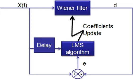
In addition, the filter length should be selected carefully, the largest size filter decreases convergence speed and vice versa. The general layout of this algorithm is shown in Figure 2:
Figure 2 Adaptive filter with LMS algorithm
2.4 Fast Block LMS algorithm:
Applying of the standard LMS algorithm to adaptive filtering results in long processing time, this due to coefficients been updated sample by sample. This delay limits the use of the LMS algorithm for real time applications, therefore the Fast Block LMS (FBLMS) algorithm was proposed to reduce the process time [41].
This algorithm is based on the transforming the time signal to the frequency domain and the filter coefficient is updated after transformation. In this algorithm
12
the filter coefficient is updated for each segment, whereas the LMS algorithm updates the coefficients for each sample. the detail procedure of FBLMS is summarised in [42].
2.5 Spectral Kurtosis and envelope analysis
Kurtosis is defined as the degree of peakness of a probability density function p(x) and mathematically it is defined as the normalized fourth moment of a probability density function [38]:
4 4 ) ( p x dx x K
(14)Where x is the signal of interest with average μ and standard deviation σ.
The basic principle of this method is to calculate the Kurtosis at different frequency bands in order to identify non stationarities in the signal and determine where they are located in the frequency domain. Obviously the results obtained strongly depend on the width of the frequency bands Δf [43]. The Kurtogram [38] is basically a representation of the calculated values of the SK as a function of f and Δf. However, the exploration of the whole plane (f, Δf) is a complicated computation task though Antoni [43] suggested a methodology for the fast computation of the SK.
On identification of the frequency band in which the SK is maximized, this information can be used to design a filter which extracts the part of the signal with the highest level of impulsiveness. Antoni et al. [29] demonstrated how the optimum filter which maximizes the signal to noise ratio is a narrowband filter at the maximum value of SK. Therefore the optimal central frequency fc and
13
bandwidth Bf of the band-pass filter are found as the values of f and Δf which maximise the Kurtogram. The filtrated signal can be finally used to perform an envelope analysis, which is a widely used technique for identification of modulating frequencies related to bearing faults. In this investigation the SK computation and the subsequent signal filtration and envelope analysis were performed using the original Matlab code programmed by Jérôme Antoni.
3
Experimental Setup
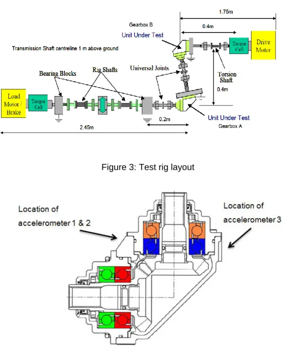
The gearbox considered is used as part of a transmission driveline on the actuation mechanism of secondary control surfaces in civil aircrafts. The test rig was designed to simulate the actual operation conditions during the life cycle of the aircraft control system which implies the gearbox would experience a range of speed and torque conditions. The test rig was driven by an electrical motor. A second motor, which acted as a generator, was employed to apply a range of loading conditions. These conditions included the simulation of takeoff and landing with different flap positions. A schematic of the testing is presented in figure 3 and load conditions are summarized in table 2. An example of a load cycle is presented for type-3 load cycle in figure 5. The motor nominal speed was 710 RPM and the expected life of the bearing under this condition is 3000 hours. The gearbox consists of two spur bevel gears as shown in figure 4, each gear with 17 teeth producing a gear ratio of 1:1. Two angular contact bearings are used to support each gear and the bearing geometric details are detailed in table 1.
During an endurance test of the flight system, a bearing within the gearbox failed after 860 hours of testing which is approximately 30% of the expected
14
bearing life. Vibration measurements were taken from the gearbox at different stages of the test. In addition, torque and angular velocity were also measured.
Figure 3: Test rig layout
15
Table 1: Bearing Geometry Bearing Geometry
No. of rolling elements (n) 12
Ball Diameter (Bd) 10.32 mm
Contact Angle (Ö) 40°
Pitch Diameter (Pd) 46 mm Input Shaft Speed (RPM) 710
Vibration data was acquired using an accelerometer fixed on the outer case of the gearbox as shown in Figure 4. The operating frequency range of the accelerometers was 10-10000 Hz. A signal conditioner (Endevco 2775A) was employed and an NI DAQ system was used to acquire data at a sampling rate of 5 KHz. Data was acquired at different periods during the endurance test.
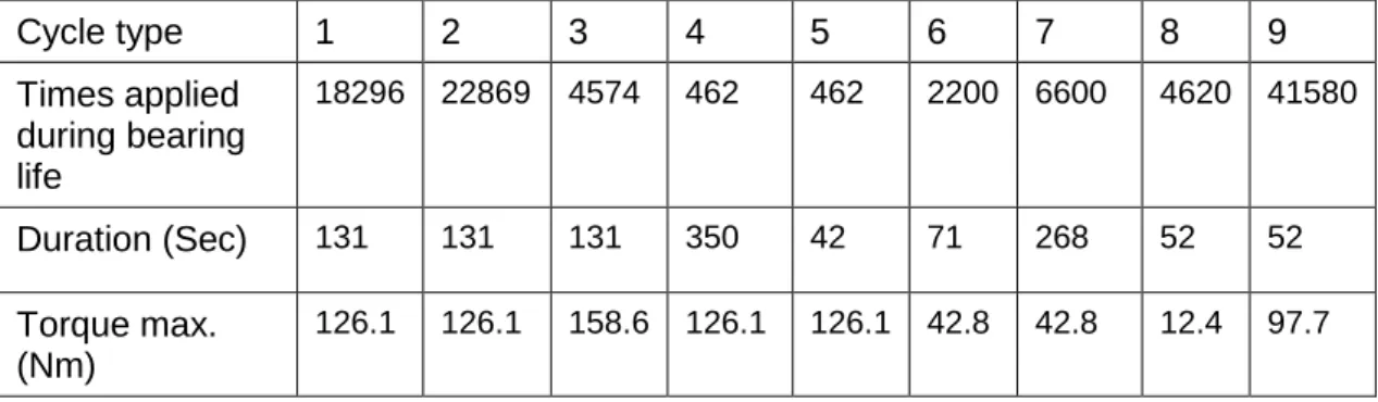
Table 2: Load cycles characteristics summary
Cycle type 1 2 3 4 5 6 7 8 9 Times applied during bearing life 18296 22869 4574 462 462 2200 6600 4620 41580 Duration (Sec) 131 131 131 350 42 71 268 52 52 Torque max. (Nm) 126.1 126.1 158.6 126.1 126.1 42.8 42.8 12.4 97.7
16
Figure 5: Example of a type 3 load cycle
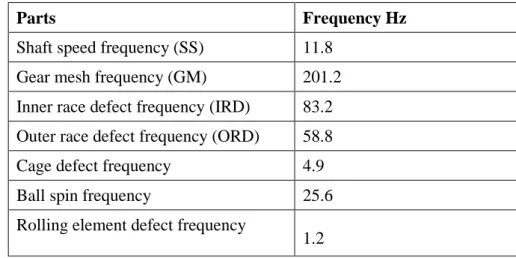
The endurance test ran continuously for 864 hours and over this period the rig was stopped at certain periods for bearing inspection after which the rig was reassembled and the test sequence resumed. Vibration data was recorded at 720, 810 and 864 hours into the endurance test corresponding to 24%, 27% and 30% of bearing life respectively. Each vibration measurement had a duration of 210 seconds sampled at 5 KHz. The duration of the vibration data represented the complete load cycle. The data under maximum torque was selected for processing. The main rotational frequencies and bearing faults frequencies are summarized in Table 3.
17
Table 3: Bearing faults frequencies
Parts Frequency Hz
Shaft speed frequency (SS) 11.8
Gear mesh frequency (GM) 201.2
Inner race defect frequency (IRD) 83.2
Outer race defect frequency (ORD) 58.8
Cage defect frequency 4.9
Ball spin frequency 25.6
Rolling element defect frequency
1.2
4
Result and Observations
4.1 Spectral Kurtosis :
Analysis employing spectral kurtosis was undertaken on all data set, this yielded the frequency band and center frequency which were then used to undertake the envelope analysis.
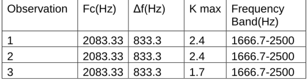
The Kurtograms spectral plots and defaults of the center frequencies are shown in Figure 6 and Table 4. These frequencies were employed for envelop analysis in this section and for enveloping the separated signal obtained from linear prediction, LMS and FBLMS algorithms.
18
First Observation Second Observation
Third Observation
Figure 6: Kurtograms of the different observations
(V
)
(V
19
Table 4: Maximum Kurtosis location
Observation Fc(Hz) Δf(Hz) K max Frequency Band(Hz)
1 2083.33 833.3 2.4 1666.7-2500
2 2083.33 833.3 2.4 1666.7-2500
3 2083.33 833.3 1.7 1666.7-2500
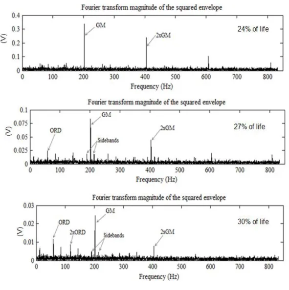
Results from enveloped analysis using the filter parameters detailed in Table 4 is presented in Figure 7. This shows clearly that the signal is dominated by the gear mesh frequency but at this point (24% of bearing life) it does not provide any information of an incipient fault in the system. In the second observation ( 27% of bearing life) a new peak at the frequency of 58.4Hz, indicating an incipient fault in the outer race of the bearing was evident. In addition, side-bands around the gear mesh frequency: 190.2Hz and 214Hz were identified. The side-bands were spaced at running speed. In third observation (30% of life ) not only was bearing outer race frequency noted but a second harmonic was also observed, see Figure 7.
20
Figure 7: Envelop spectrum using parameters from SK
4.2 Linear prediction Result
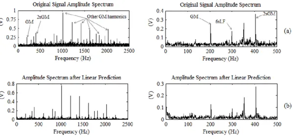
Signal separation with linear prediction was undertaken on vibration data measured at 720 hrs into the endurance test. Following separation the frequency spectrum of the determinate part of vibration signature was undertaken. From the analysis, and observations of Figure 8, it was observed
21
that the background noise reduced following Linear Prediction with a relative increase in SNR of 2.6%, however, no bearing defect frequencies were identified in the frequency spectrum but the dominance of the gear mesh frequency (201 Hz) was noted.
Figure 8 First observation spectrum using original signal and linear prediction
The second observation measured at 810 hrs, approximately 27% of bearing life, showed a frequency spectrum similar to that noted at 720 hrs (see Figure 9), with the difference being that there is a reduction in the amplitude of the peaks and the background noise is slightly lower. No new fault frequencies were identified in the frequency spectrum following Linear Prediction, despite the fact that the SNR improved by 14% in the signal to noise ratio.
22
Figure 9: Spectrums at second observation using original signal and linear prediction
Following analysis at 840 hours (30% of bearing life) observations showed that the amplitude of the various frequency components in the spectrum is relatively lower than noted earlier (see Figure 10). This is due to the fact that this measurement was taken during a loading cycle where the transmitted torque was lower (40 Nm) than in the previous measurements (126 Nm). Even under this low torque conditions and despite the reduction in amplitude, all previously noted peaks in the spectrum were evident, in addition to a clear peak at 58.8HZ, indicating the defect in the outer race of the bearing.
23
Figure 10: Spectrums at third observation
4.3 LMS and FBLMS result
The Adaptive filter was applied to the measured bearing vibration signature at different stages of the endurance test, both LMS and FBLMS algorithms were applied to perform signal separation, the result of each algorithm will be compared later.
In order to ensure the convergence of the algorithm, the Mean Square Error (MSE) was estimated, the adaptive filter with minimum and stable MSE represents the best solution for signal separation, the filter length is selected as 2000 and step size of 0.00001 based on equation (13) and minimum MSE as shown in convergence curve in figure 11.
24
Figure 11 Learning curve for LMS algorithm
After the bearing signal separation had been completed, envelop analysis was performed to identify any bearing defect frequencies. The envelop analysis was performed by applying a band-pass filter centered around 2083 HZ with a bandwidth of 833.33 HZ. These parameters were selected based on the result from maximum Spectral Kurtosis as described in section 4.1.
The spectrum of enveloped signal associated with 24% of bearing life is presented in Figure 12 for the LMS algorithm. Observations showed the gear mesh (201.1 Hz) was dominant ( see left plot in figure 12). The right plot in Figure 12 represents a narrower frequency range in the original spectrum showing the presence of BPFO, shaft speed and harmonics of shaft speed. Figure 13 shows the result obtained by enveloping the FBLMS algorithms, which doesn’t show the existence of any fault frequencies at this stage.
25
Figure 12 Enveloped signal spectrum with LMS algorithm at 24% of life
Figure 13: Enveloped signal spectrum using a FBLMS algorithm at 24%
V rm s^2 V rms ^2 Frequency Frequency
26
The spectrum of the enveloped signal from the second data (27% of bearing life) using the LMS algorithm is shown in figure 14. The presence of the outer race defect frequency was evident; in addition a second harmonic of the BPFO was noted (118 Hz). This result supports the observation obtained from the first data set ( see figure 12). Furthermore, the bearing inner race defect was also identified at 83.2 Hz as shown in figure 14 .
Result from processing the data at 27% using FBLMS algorithms showed the presence of both BPFI and BPFO frequencies at 58.85 and 83.2 HZ respectively, see figure 15. In addition, side-bands around gear mesh spaced by shaft frequency and shaft harmonics were identified by both algorithms as shown in figure 14 and figure 15.
Figure 14: Enveloped signal spectrum with LMS algorithm at 27% of life
V
rm
s^
27
Figure 15: Enveloped signal spectrum with FBLMS algorithm at 27% of life For data set collected at 30% of bearing life, the frequency spectrum obtained from the LMS algorithms showed BPFO, BPFI, and Ball Spin (BS) frequencies, see figure 16. In addition the second harmonic of the BPFI frequency (165 Hz) was evident. The frequency spectrum obtained from the FBLMS algorithms showed BPFI and BPFO frequencies as shown in figure 17. In both algorithms, the amplitude of BPFO decreased by 14% from the previous data set; this is attributed to an increase of bearing clearances due to defects which result in a decrease of bearing vibration. In addition, this data was recorded during a loading cycle where the transmitted torque (50 Nm) was lower than in the previous measurements (126 Nm) . Figure 16 and figure 17 show Sidebands around fundamental gear mesh spaced by shaft frequency and shaft harmonics were now more pronounced in the spectrum for the data set associated with 30% bearing life, this is indicative of misalignment. This misalignment can affect the gear mesh and further accelerate bearing degradation, consequently the test was stopped at this stage and a visual inspection was performed to assess the damage.
V
rm
s^
28
Figure 16: Enveloped signal at 30% of life using LMS algorithm
Figure 17: Enveloped signal spectrum at 30% of life using FBLMS algorithm At all three life stages the gearbox was disassembled for visual inspection, evidence of scratches in the bearing outer race at an early stage of 24 % was observed, see figure 18. At the end of the test the bearing ball and outer race were damaged as shown in figure 19.
V rm s^2 V rm s^2
29
Figure 18 bearing failure progress at 24% and 30% of life time
Figure 19 Inner race damaged at the end of the test 24%
30
5
Discussion
The techniques used in this paper are typically used for applications where strong background noise masks the defect signature of interest within the measured vibration signature. Of all the techniques presented, the LMS algorithm succeeded in detecting the bearing outer race fault earliest at 24% of bearing life. FBLMS and SK techniques detected the bearing outer race fault at 27% of bearing life. In addition, the LMS algorithm was the only technique that successfully identified both the outer race and ball spin faults. The Linear Prediction algorithm detected the fault at 30% of bearing life, though Linear Prediction showed its capability in reducing the background noise and facilitating the identification of the different components in the signal spectrum. Comparing the LMS and FBLMS algorithms showed that LMS is able to detect the bearing fault earlier than FBLMS. However, the computational cost for LMS is high and therefore FBLMS is more suitable for online diagnostics where an immediate response is required. On the other hand, LMS can be used for offline diagnostics. However, with today’s computer technology the delay time can be reduced significantly to a few minutes. In some applications such as wind and tidal turbines, vibration data is acquired once every hour depending on certain conditions. This makes the LMS algorithm the best candidate for diagnosing bearing faults in gearboxes.
31
6
Conclusion:
The problem of bearing fault diagnosis in gearboxes has been investigated; Linear Prediction, Spectral Kurtosis, LMS and FBLMS algorithms were applied to separate the bearing signal. The LMS technique demonstrated the ability to identify the defect earlier than all other methods. This method is thus a very powerful tool for early fault detection in bearings, particularly for those applications where strong background noise from other sources in the machine masks the characteristics fault components in the frequency domain.
32 References
[1] Randall, R. B. and Antoni, J. (2011), "Rolling element bearing diagnostics A tutorial", Mechanical Systems and Signal Processing, vol. 25, no. 2, pp. 485-520.
[2] Halim, E. B., Shah, S. L., Zuo, M. J. and Choudhury, M. A. A. (2006), "Fault detection of gearbox from vibration signals using time-frequency domain averaging", American Control Conference, 2006, pp. 6 pp.
[3] Tan, C. K., Irving, P. and Mba, D. (2007), "A comparative experimental study on the diagnostic and prognostic capabilities of acoustics emission, vibration and spectrometric oil analysis for spur gears", Mechanical Systems and Signal Processing, vol. 21, no. 1, pp. 208-233.
[4] Behzad, M., Bastami, A. R. and Mba, D. (2011), "A new model for estimating vibrations generated in the defective rolling element bearings", Journal of Vibration and Acoustics, Transactions of the ASME, vol. 133, no. 4.
[5] Li, Z., Yan, X., Tian, Z., Yuan, C., Peng, Z. and Li, L. (2013), "Blind vibration component separation and nonlinear feature extraction applied to the nonstationary vibration signals for the gearbox multi-fault diagnosis", Measurement, vol. 46, no. 1, pp. 259-271.
[6] Randall, R. B. and Tech, B. (2004), "Cepstrum Analysis and Gearbox Fault Diagnosis", [Online], no. 2nd edition, pp. 10/07/2012 available at: www.bksv.com/doc/233-80.pdf.
[7] Al-Ghamd, A. M. and Mba, D. (2006), "A comparative experimental study on the use of acoustic emission and vibration analysis for bearing defect identification and estimation of defect size", Mechanical Systems and Signal Processing, vol. 20, no. 7, pp. 1537-1571.
[8] McFadden, P. D. and Toozhy, M. M. (2000), "Application of Synchronous Averaging to Vibration Monitoring of rolling elements bearings", Mechanical Systems and Signal Processing, vol. 14, no. 6, pp. 891-906.
33
[9] Fu-cheng, Z. (2010), "Research on online monitoring and diagnosis of bearing fault of wind turbine gearbox based on undecimated wavelet transformation", Information Computing and Telecommunications (YC-ICT), 2010 IEEE Youth Conference on, pp. 251.
[10] Howard, I. (1994), A review of rolling element bearing vibration '' Detection, Diagnosis and Prognosis'', DSTO-RR-0013, Department of defense.
[11] Wang, W. J. and McFadden, P. D. (1993), "Early detection of gear failure by vibration analysis i. calculation of the time-frequency distribution", Mechanical Systems and Signal Processing, vol. 7, no. 3, pp. 193-203. [12] Sawalhi, N., Randall, R. B. and Endo, H. (2007), "The enhancement of
fault detection and diagnosis in rolling element bearings using minimum entropy deconvolution combined with spectral kurtosis", Mechanical Systems and Signal Processing, vol. 21, no. 6, pp. 2616-2633.
[13] Randall, R. B. (2004), "Detection and diagnosis of incipient bearing failure in helicopter gearboxes", Engineering Failure Analysis, vol. 11, no. 2, pp. 177-190.
[14] McFadden, P. D. and Smith, J. D. (1984), "Vibration monitoring of rolling element bearings by the high-frequency resonance technique — a review", Tribology International, vol. 17, no. 1, pp. 3-10.
[15] McFadden, P. D. (1987), "A revised model for the extraction of periodic waveforms by time domain averaging", Mechanical Systems and Signal Processing, vol. 1, no. 1, pp. 83-95.
[16] Randall, R. B., Sawalhi, N. and Coats, M. (2011), "A comparison of methods for separation of deterministic and random signals", The International Journal of Condition Monitoring, vol. 1, no. 1, pp. 11.
[17] Barszcz, T. (2009), "Decomposition of vibration signals into deterministic and nondeterministic components and its capabilities of fault detection and identification", International Journal of Applied Mathematics and Computer Science, vol. 19, no. 2, pp. 327-335.
34
[18] Carney, M. S., Mann III, J. A. and Gagliardi, J. (1994), "Adaptive filtering of sound pressure signals for monitoring machinery in noisy environments", Applied Acoustics, vol. 43, no. 4, pp. 333-351.
[19] Khemili, I. and Chouchane, M. (2005), "Detection of rolling element bearing defects by adaptive filtering", European Journal of Mechanics - A/Solids, vol. 24, no. 2, pp. 293-303.
[20] Antoni, J. and Randall, R. B. (2004), "Unsupervised noise cancellation for vibration signals: part I—evaluation of adaptive algorithms", Mechanical Systems and Signal Processing, vol. 18, no. 1, pp. 89-101.
[22] Satorius, E. H., Zeidler, J. R. and Alexander, S. T. (1979), "Noise cancellation via linear prediction filtering", Acoustics, Speech, and Signal Processing, IEEE International Conference on ICASSP '79. Vol. 4, pp. 937. [23] Thakor, N. V. and Zhu, Y. (1991), "Applications of adaptive filtering to
ECG analysis: noise cancellation and arrhythmia detection", Biomedical Engineering, IEEE Transactions on, vol. 38, no. 8, pp. 785-794.
[24] Chaturved, G. K. and Thomas, D. W. (1981), "Adaptive noise cancelling and condition monitoring", Journal of Sound and Vibration, vol. 76, no. 3, pp. 391-405.
[25] Ho, D. and Randall, R. B. (2000), "Optimisation of bearing diagnostic techniques using simulated and actual bearing fault signal", Mechanical Systems and Signal Processing, vol. 14, no. 5, pp. 763-788.
[26] Antoni, J. and Randall, R. B. (2001), "optimisation of SANC for Separating gear and bearing signals", Condition monitoring and diagnostics engineering management, , no. 1, pp. 89-99.
[27] Widrow, B., Glover, J. R., Jr., McCool, J. M., Kaunitz, J., Williams, C. S., Hearn, R. H., Zeidler, J. R., Eugene Dong, J. and Goodlin, R. C. (1975), "Adaptive noise cancelling: Principles and applications", Proceedings of the IEEE, vol. 63, no. 12, pp. 1692-1716.
[28] Simon, H. (1991), Adaptive Filter theory, Second ed, Prentice-Hall international, Inc, USA.
35
[29] Antoni, J. and Randall, R. (2006), "The spectral kurtosis: application to the vibratory surveillance and diagnostics of rotating machines", Mechanical Systems and Signal Processing, vol. 20, no. 2, pp. 308-331.
[30] Dwyer, R. (1983), "Detection of non-Gaussian signals by frequency domain kurtosis estimation", Acoustics, Speech, and Signal Processing, IEEE International Conference on ICASSP'83. Vol. 8, IEEE, pp. 607.
[31] Douglas, S. C. (1999), Introduction to Adaptive Filters, CRC Press.
[32] Douglas, S. C. and Rupp, M. (1999), "Convergence Issues in the LMS Adaptive Filter", in Madisetti, V. K. (ed.) The Digital signal processing handbook, Second ed, CRC press, Atlanta, USA.
[33] Widrow, B., McCool, J. and Ball, M. (1975), "The complex LMS algorithm", Proceedings of the IEEE, vol. 63, no. 4, pp. 719-720.
[34] Gardner, W. A. (1978), "Stationarizable random processes", Information Theory, IEEE Transactions on, vol. 24, no. 1, pp. 8-22.
[35] Gardner, W. A. and Franks, L. (1975), "Characterization of cyclostationary random signal processes", Information Theory, IEEE Transactions on, vol. 21, no. 1, pp. 4-14.
[36] Makhoul, J. (1975), "Linear prediction: A tutorial review", Proceedings of the IEEE, vol. 63, no. 4, pp. 561-580.
[37] Yule, G. U. (1927), "On a method of investigating periodicities in disturbed series, with special reference to Wolfer's sunspot numbers", Philosophical Transactions of the Royal Society of London.Series A, Containing Papers of a Mathematical or Physical Character, vol. 226, pp. 267-298.
[38] Randall, R. B. (2011), Vibration-based Condition Monitoring, first ed, John Wiley and sons Ltd, UK.
[39] Wang, W. (2008), "Autoregressive model-based diagnostics for gears and bearings", Insight-Non-Destructive Testing and Condition Monitoring, vol. 50, no. 8, pp. 414-418.
36
[40] Ljung, L. (1999), "<br />Linear Regressions and Least Squares", in System identification: Theory for the user, 2nd ed, Pentrice-Hall, New Jersey, pp. 321-324.
[41] Dentino, M., McCool, J. and Widrow, B. (1978), "Adaptive filtering in the frequency domain", Proceedings of the IEEE, vol. 66, no. 12, pp. 1658-1659.
[42] Ferrara, E. R. (1980), "Fast implementations of LMS adaptive filters", Acoustics, Speech and Signal Processing, IEEE Transactions on, vol. 28, no. 4, pp. 474-475.
[43] Antoni, J. (2007), "Fast computation of the kurtogram for the detection of transient faults", Mechanical Systems and Signal Processing, vol. 21, no. 1, pp. 108-124.
[44] Li, H., Zhang, Y. and Zheng, H. (2009), "Gear fault detection and diagnosis under speed-up condition based on order cepstrum and radial basis function neural network", Journal of Mechanical Science and Technology, vol. 23, no. 10, pp. 2780-2789.