An application of extreme value theory in medical sciences

UNIVERSIDADE DE LISBOA FACULDADE DE CIÊNCIAS

DEPARTAMENTO DE ESTATÍSTICA E INVESTIGAÇÃO OPERACIONAL

An application of extreme value theory in medical

sciences

Constantino Pereira Caetano

Mestrado em Bioestatística

Dissertação orientada por:

Professora Doutora Patrícia de Zea Bermudez

Acknowledgements

In no special order, I would like to profoundly thank the following individuals and institutions for helping me realize this lifelong dream.

To my mother, for inspiring me to pursue a scientific career and giving me the possibility to do so. To my step-father, for the excellent mathematical input into my work.

To my father, with whom I had the most fascinating mathematical discussions that inspired me to pursue this journey.

To my advisor, Professor Patrícia de Zea Bermudez, who presented me with the most interesting challenges throughout this dissertation.

To my friend João Torrado, for giving me a place to stay and being a friend to debate statistics with. To Dr. Eduardo Gomes da Silva, head of medicine of Serviço de Medicina 3.2 of the Hospital dos Capuchos, Lisbon, who offered an afternoon of his time to answer my questions about blood pressure and its pathologies.

To the Department of Pharmaceutical Care Services of the Portuguese National Association of Phar-macies (ANF), for enabling me the use of the data used in this thesis.

Resumo

Valores altos de pressão arterial são considerados um fator de risco de doenças cardiovasculares, ver [Hajar, 2016]. Estas doenças são a principal causa de morte em Portugal. Com o objectivo de criar um perfil da população Portuguesa em relação aos riscos de doenças cardiovasculares, um estudo foi desenvolvido em 2005, pela Associação Nacional de Farmácias através do seu Departamento de Serviços Farmacêuticos. O interesse principal do presente estudo consiste em modelar valores eleva-dos de pressão arterial sistólica em indivíduos que sofrem de uma categoria particular de hipertensão. Um estudo similar foi desenvolvido para modelar os valores elevados de níveis de colesterol total, ver [de Zea Bermudez and Mendes, 2012]. A presente dissertação tem dois principais interesses: estudar a distribuição geográfica dos valores elevados de pressão arterial sistólica (em indivíduos com valores normais de pressão arterial diastólica) em Portugal, i.e., ajustar modelos de valores extremos para cada distrito de Portugal e ilhas e analisar em particular o grupo de maior risco, i.e., indivíduos idosos. Com

esse propósito, a metodologiaPeaks Over Thresholdfoi aplicada. Esta metodologia consiste em ajustar

um modelo aos excessos (ou excedências) acima de um limiar de pressão arterial sistólica

suficiente-mente elevado. Os modelos obtidos serão capazes de estimar quantis elevados e probabilidades decauda

de pressão arterial sistólica.

Na presente dissertação, os indivíduos foram divididos em quatro grupos distintos. Aqueles que apresentavam valores normais de pressão arterial sistólica e pressão arterial diastólica. Os que apresen-tavam valores superiores aos delineados pelas entidades médicas em um ou ambos os índices, ver tabela 6.1. Dentro deste último grupo consideramos os indivíduos que sofrem de hipertensão arterial sistólica isolada, caracterizada por valores de pressão arterial sistólica superior ou igual a 140 mmHg e valor de pressão arterial diastólica inferior a 90 mmHg. Pretendemos estudar valores elevados de pressão arterial sistólica neste grupo.

Em primeira análise, foi efectuado um estudo descritivo dos indivíduos que frequentaram a campanha e que sofrem de hipertensão sistólica isolada, com o intuito de averiguar o efeito de outras variáveis de interesse nos níveis de pressão arterial sistólica. As variáveis consideradas nesta analise preliminar foram a idade, cuja relação com valores elevados de pressão arterial sistólica é conhecida, ver [Pinto, 2007]; o género, consumo de tabaco, índice de massa corporal e distrito.

A análise de valores extremos utilizando a metodologia Peaks Over Threshold consiste em

vá-rias etapas. Em primeiro lugar, é necessário obter o valor limiar elevado (threshold) com o objectivo de ajustar uma distribuição generalizada de Pareto aos seus excessos. Esta distribuição tem

parâme-tro de forma k e parâmetro de escala σ, ver expressão (3.2). Esta primeira etapa é por vezes

difí-cil. A literatura apresenta várias metodologias para tratar esta fase. Existem métodos exploratórios, como o descrito por [Coles, 2001], que utiliza a função de excesso médio para discernir o limiar

ele-vado pretendido. [DuMouchel, 1983] sugere utilizar χ0.9 como valor limiar. Existem também

mé-todos que consistem em ajustar o modelo considerando vários valores limiar e avaliar qual produz o melhor ajustamento, como por exemplo os testes de Cramér-von Mises e Anderson-Darling, ver [Choulakian and Stephens, 2001]. Ainda dentro deste grupo destacamos um método Bayesiano que uti-liza medidas de surpresa, ver [Lee et al., 2015]. Todos os métodos referidos acima são utiuti-lizados ao longo da dissertação.

Após concluída esta fase procedemos ao ajuste de uma distribuição generalizada de Pareto aos ex-cessos do valor limiar seleccionado. Máxima verosimilhança é a metodologia mais usual para efectuar o

ajustamento visto que os resultantes estimadores dos parâmetros gozam de propriedades relevantes.

Numa primeira etapa, implementamos a metodologiaPeaks Over Threshold nos indivíduos que

so-frem de pressão arterial sistólica isolada em cada distrito de Portugal continental e ilhas. Aqui são exploradas as dificuldades inerentes na análise de valores extremos e também alguns problemas encon-trados nos dados, os quais são explorados no capítulo seguinte, onde analisamos os valores de pressão arterial sistólica em indivíduos idosos, (idade superior ou igual a 55) e consideramos um método que trata o problema de testes múltiplos para hipóteses ordenadas. Estas resultam da aplicação dos testes de Cramér-von Mises e Anderson-Darling para diferentes partições da amostra; e consideramos também

modelosjitteringpara lidar com o problema de discretização dos dados.

Palavras-chave: Teoria de Valores Extremos, Estatística Bayesiana, ModelosThreshold, Escolha de

Abstract

It has been well stated that high values of blood pressure constitute a risk factor for cardiovascular diseases [Hajar, 2016], with the latter being the number one death cause in Portugal. With the objective of profiling the Portuguese population in what regards cardiovascular diseases’ risk factors, a study was developed and carried out in 2005, by the National Pharmacy Association through its Department of Pharmaceutical Care. The main interest of the present study is to model the high values of systolic blood pressure of individuals with a specific hypertension pathology. A similar study was developed for the total cholesterol levels [de Zea Bermudez and Mendes, 2012]. The aims of this dissertation are twofold: to study the geographical distribution of the high systolic blood pressure (but normal diastolic blood pressure) in Portugal, i.e., fitting extreme value models for each Portuguese district and islands

and studying the group that is more at risk, i.e., the elderly. With that purpose, thePeaks Over Threshold

methodology was applied, which consists in finding a sufficiently high systolic blood pressure threshold and fitting a tail model to the excesses. The models will be able to estimate extreme quantiles and tail probabilities of the systolic blood pressure in each group.

Keywords: Extreme Value Theory, Bayesian Statistics, Threshold Models, Threshold Selection, Multiple Testing For Ordered Hypotheses.

Contents

1 Introduction 1

2 Models for Extreme Values 3

2.1 Introduction . . . 3

2.2 Classical Extreme Value Theory . . . 3

3 Threshold Models 5 3.1 Introduction . . . 5

3.2 The Generalized Pareto Distribution . . . 5

3.3 The Generalized Pareto Distribution and Threshold Models . . . 6

3.4 Methods for Threshold Selection . . . 7

3.4.1 Mean Residual Life Function . . . 7

3.4.2 Goodness-of-fit Tests for the Generalized Pareto Distribution . . . 8

3.4.3 Bayesian Method for Threshold Selection . . . 9

3.5 The Peaks Over Threshold Methodology . . . 11

3.5.1 Maximum Likelihood Estimation . . . 11

3.5.2 Estimation of Extreme Quantiles . . . 12

4 Basics of Bayesian Statistics 15 4.1 Bayes’ Theorem . . . 16

4.1.1 The Discrete Case . . . 16

4.1.2 The Continuous Case . . . 16

4.2 Predictive Posterior Distribution . . . 17

4.3 Bayes’ Factor . . . 17

4.4 Predictivep-values . . . 18

5 The Delta Method 19 6 Descriptive Analysis of the Biometric Variables Recorded in Portuguese Voluntary Phar-macy Attendees 22 6.1 Introduction . . . 22

6.2 Exploratory Data Analysis . . . 23

7 First Approach to Extreme Value Modeling of Systolic Blood Pressure Values 29 7.1 Data Description and Methodologies . . . 29

7.2 Model Fitting . . . 30

8 Modeling Extreme Systolic Blood Pressure Values in the Elderly 41

8.1 Jitter and Non-jitter Extreme Value Models for Systolic Blood Pressure in Individuals

Who Suffer From Isolated Systolic Hypertension . . . 42

8.2 Threshold Selection Analysis . . . 46

9 Comments, Conclusions and

List of figures

3.1 Mean residual life plot for the dataset simulated from a mixture distribution . . . 8

3.2 Histogram of the mixture model . . . 10

3.3 Plotted predictive p-values from a mixture distribution for an array of ordered thresholds 11 6.1 Diastolic blood pressurevs.systolic blood pressure for Portuguese voluntary pharmacy attendees . . . 23

6.2 Systolic blood pressure boxplots by gender(left)and by tobacco consumption(right) . . 24

6.3 Systolic blood pressure boxplots by age strata . . . 25

6.4 Systolic pressure by BMI strata . . . 26

6.5 Systolic blood pressure by Portuguese district . . . 27

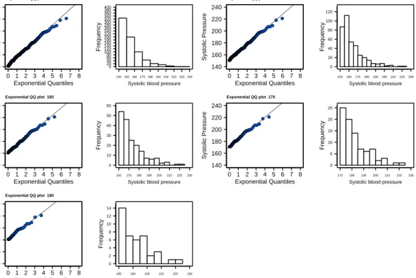
7.1 Exponential QQ-plots and histograms for an array of thresholds for Braga . . . 30

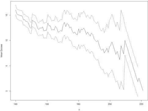
7.2 Estimated mean residual life function for the Braga district . . . 31

7.3 Bayesian method for threshold selection using measure of surprise . . . 31

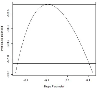
7.4 Profile likelihood function for the shape parameter . . . 33

7.5 Estimated kernel density function of the observed systolic blood pressure values for in-dividuals who suffer from isolated systolic hypertension . . . 36

7.6 Estimated kernel density function of the observed systolic blood pressure values for in-dividuals who suffer from isolated systolic hypertension for the district of Coimbra . . . 37

7.7 Bayesian method for threshold selection using measures of surprise for Coimbra’s ob-servations of systolic blood pressure. . . 37

7.8 Estimated kernel density function of the observed systolic blood pressure values for in-dividuals who suffer from isolated systolic hypertension for the district of Braga . . . 40

8.1 Estimated kernel density function of the observed systolic blood pressure values for el-derly individuals who suffer from isolated systolic hypertension . . . 42

8.2 Kernel density function estimation for a sample generated from a beta(10,10,-0.5,0.5) distribution (n=8174) . . . 43

8.3 Kernel density function estimation for a sample generated from a uniform(-1.5,1.5) dis-tribution (n=8174) . . . 43

8.4 Histograms and kernel density estimation for the non-jitter data and jitter data using the uniform and beta distributions . . . 44

8.5 Exponential QQ-plots and histograms for each candidate threshold for the non-jitter data 45 8.6 Exponential QQ-plots and histograms for each candidate threshold for the uniform-jitter data . . . 45

8.7 Exponential QQ-plots and histograms for each candidate threshold for the beta-jitter data 46 8.8 Mean residual life function for the non-jitter data . . . 47

8.9 Mean residual life function for the uniform-jitter data . . . 47

8.10 Mean residual life function for the beta-jitter data . . . 48

8.11 Bayesian threshold selection method using measure of surprise for the non-jitter, uniform-jitter and beta-uniform-jitter data . . . 48

8.12 Density plots with histogram and profile likelihood plots for the non-jitter (left),

List of tables

4.1 Bayes’ factor output interpretation by [Kass and Raftery, 1995] . . . 18

6.1 Categories of blood pressure in mmHg (Portuguese Cardiology Association guidelines) . 23

6.2 Summary statistics of the systolic blood pressure in men and women who suffer from

isolated systolic hypertension . . . 24

6.3 Summary of the systolic pressure by age in Portuguese voluntary pharmacy attendees

who suffer from isolated systolic hypertension . . . 25

6.4 BMI classes . . . 26

6.5 Summary of the systolic blood pressure by BMI strata in Portuguese voluntary pharmacy

attendees who suffer from isolated systolic hypertension . . . 27

6.6 Summary statistics of systolic blood pressure by Portuguese district and islands . . . 28

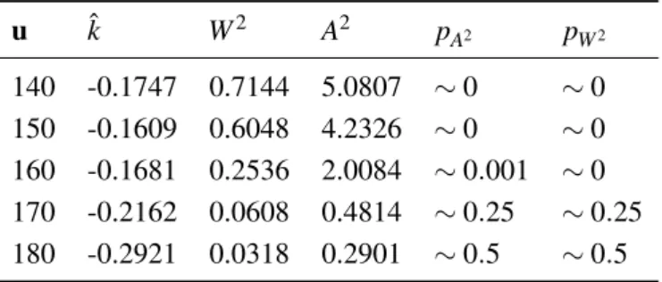
7.1 Cramér-von Mises and Anderson-Darling hypothesis testing for the Braga district . . . . 32

7.2 Model fitted to Braga . . . 32

7.3 Result of the deviance test for Braga . . . 33

7.4 Fitted GPD models to each Portuguese district and islands . . . 34

7.5 Extreme quantiles for each Portuguese district and islands. Empirical estimates forq0.995

are not included since for some districts there are few observations above this value. (*)

values greater than 300 mmHg . . . 38

7.6 Extreme quantiles for each Portuguese district and islands using the exponential model.

Empirical estimates for q0.995 are not included since for some districts there are few

observations above this value . . . 39

7.7 Cramér-von Mises e Anderson-Darling goodness-of-fit test for the GPD for the values of

SBP in Braga . . . 40

8.1 Summary of the systolic blood pressure by age in the uniform jitter-data, beta-jitter data

and non-jitter data . . . 44

8.2 Results of the automated threshold selection using the Cramér-von Mises goodness-of-fit

tests for the non-jitter dataset . . . 49

8.3 Results of the automated threshold selection using the Cramér-von Mises goodness-of-fit

tests for the uniform jitter dataset . . . 49

8.4 Results of the automated threshold selection using the Cramér-von Mises goodness-of-fit

tests for the beta-jitter dataset . . . 49

8.5 Extreme models for the non-jitter, beta-jitter and uniform-jitter data. (∗) the support does

not have an upper finite boundary . . . 50

8.6 Results of the deviance test for non-jitter model, uniform-jitter model and beta jitter-model 51

8.7 Extreme quantiles for the uniform-jitter model, beta-jitter model and non-jitter model . . 51

8.8 Extreme quantiles for the uniform-jitter model, beta-jitter model and non-jitter model

1

|

Introduction

Extreme events can be defined as low frequency episodes of some apparently random process. For example, floods transpire when the water level of some water body exceeds an uncommonly high th-reshold. Classical statistical methodologies are not suited to treat this kind of data, since they aim to make predictions about future behavior of the treated phenomena based on the most common events, i.e., classical statistics uses the centralized data to infer on future behavior by fitting the data to models based on asymptotic central limit like results. Such an approach might be considered too overly simplified to infer on rare events. Hence, the extreme value analysis paradigm arose out of the necessity to treat data that falls on this scope. It offers well suited statistical procedures to describe the tail distribution behavior of the underlying data creation process.

Extreme value theory (EVT) can be applied to an assortment of different scientific and economic branches, ranging from meteorology, hydrology and insurance, amongst others. It was introduced by Leonard Tippett (1902-1985) and Sir Ronald Aylmer Fisher (1890-1962). Tippett worked for the British cotton industry research association where he developed research to make the cotton threads stronger. He showed that the cotton thread is only as strong as its weakest fibers. Along with Fisher, Tippet laid the probabilistic frameworks of what became the extreme value theory as it is known today. Gumbel was also an outstanding contributer to the development of EVT, see [Gumbel, 1935].

Like classical statistics, EVT aims to fit known statistical models to the data. Since the interest is to fit models to the least common data, it is natural to consider models for the tail of the distribution. These were first introduced by Fisher and Tippet. They proved that, under the criteria of independent and identically distributed (i.i.d.) random variables, the sample maxima (or minima) could be modeled by one of three tail distributions of extremes as the sample size increases. This method is widely known

in the literature as theAnnual Maxima.

Other methods include thePeaks Over Thresholdapproach (POT). This methodology aims to fit a

tail-like model to the excesses over a high threshold. It was first developed by [Pickands, 1975] and [Balkema and de Haan, 1974]. Research into POT models is an ongoing topic. In this dissertation, we use several recently developed methods that provide further evidence in selecting the most suited th-reshold model for the data.

One of the most strenuous analysis using POT is the selection of the threshold value, i.e., the value over which the tail-like distribution model is fitted. We address several recent methods pertaining to this analysis, see [Lee et al., 2015], [Bader et al., 2018] and [Coles, 2001].

Models obtained by using EVT techniques are able to extrapolate on the likelihood of future extreme events, even if such events were not observed during the sampling process. For example, if one were to record Lisbon’s precipitation levels each day for a long period of time during the rainy season, one might never observe a flood or a dry spell. Though the data could be fitted to an EVT model that could extrapolate the likelihood of observing such events, the interest might also lie in finding the value that is exceeded, in mean, once every rainy season, which the latter also foresees.

Although not common, EVT can be used to treat medical data. Furthermore, some literature exists on this topic, [de Zea Bermudez and Mendes, 2012] fit EVT models to the total cholesterol recorded of Por-tuguese voluntary pharmacy attendees. In this dissertation we use POT techniques to fit threshold models to systolic blood pressure data. We use a database obtained during a study of risk factors associated with cardiovascular diseases in the Portuguese population, where in certain Portuguese pharmacies, voluntary

attendees had several biometric variables recorded, such as total cholesterol, triglycerides, systolic blood pressure, diastolic blood pressure and body mass index, amongst others.

Hypertensive individuals have a higher risk rate of contracting heart diseases, see [Hajar, 2016]. With the objective of analyzing this health issue in Portugal, a campaign was carried out by the National Pharmacy Association through its Department of Pharmaceutical Care in 2005, with the goal of iden-tifying individuals at risk. This dissertation aims to study individuals who suffer from isolated systolic hypertension (ISH), that is, individuals that have systolic blood pressure higher or equal to 140 mmHg and diastolic blood pressure lesser than 90 mmHg (current guidelines from the Portuguese Hypertension Society).

In the first chapters of this dissertation we outline the main EVT theorems and results. We delve more into the intricacies of the threshold models, where we formulate the POT’s asymptotic distribution of ex-cesses (or exceedances) above a sufficiently high threshold. This will be the main methodology applied throughout this dissertation. We then present several methods for threshold selection, namely an explo-ratory method using the mean residual life function as described by [Coles, 2001] and one method using goodness-of-fit hypotheses testing for the generalized Pareto distribution (GPD), with a rule to account for multiple ordered hypotheses testing, see [Choulakian and Stephens, 2001] and [Bader et al., 2018]. We also include a beginner’s guide to Bayesian statistics, since one of the methods proposed for threshold

selection requires some knowledge on this domain. This state-of-the-art method uses the predictive p

-value obtained by sampling from the predictive posterior distribution to calculate tail-area probabilities

by considering a range of threshold candidates. These p-values can be interpreted so that a suited

th-reshold is selected. The R code used in this dissertation for the application of this method was courte-ously made available by the authors who developed it, see [Lee et al., 2015]. Chapter 5 presents the basic concept of the delta method which will be used in subsequent chapters.

Chapter 6 presents the exploratory analysis of the individuals who volunteered to join the campaign. Several variables were examined alongside systolic blood pressure, such as age, body mass index, gender and district.

Chapter 7 and 8 pertain to the extreme value modeling of systolic blood pressure for the previously mentioned individuals who suffer from ISH. We perform a first approach for each Portuguese district using these methods, highlighting the difficulties involved with the threshold model analysis. On a

second stage, we model the systolic pressure of the elderly individuals (>=55) who suffer from ISH,

with the objective of applying more rigorous statistical analysis to obtain better suited models. This group is of particular interest, since elderly people have a higher prevalence of ISH [Bavishi et al., 2016].

2

|

Models for Extreme Values

2.1

Introduction

In today’s modernized and highly technological world, it is imperative to study the risk of extreme events associated with economical and natural disasters, such as the 2008 Wall Street stock market crash and Hurricane Maria that devastated Puerto Rico in 2017. The likelihood of these events is very low, meaning that if they were quantified through standard statistical analysis, they would fall on the tail-end of the distribution.

Let’s consider total rainfall as an example. We are interested in assessing the amount of rainfall that is needed to cause a flood and not the usual mild rain. This amount in not usually observed, hence being termed a rare event. Extreme value analysis offers well suited statistical techniques capable of predicting these events. It outlines statistical procedures to predict certain quantities of interest, such as

the most extreme value of a given distribution known asendpoint(if it is finite), the probability of some

extreme value being exceeded, termedtail probabilityand extreme quantile estimation ortail quantiles,

i.e., values that have a low probability of being exceeded.

In this chapter we explore the asymptotic frameworks of classical extreme theory.

2.2

Classical Extreme Value Theory

Although there is some literature on sequences of dependent variables for extreme value analysis, this setting does not fall under the scope of this thesis. [Coles, 2001] has a chapter dedicated to this topic. Hence we consider the standard sequence of independent variables with common distribution. Let

X be a random variable with distribution functionF and

Mn = max(X1,X2, ...,Xn), (2.1)

whereX1,X2, ...,Xnrepresents a random sample ofX. The aim is to study the distribution ofMn. We can

derive this distribution as follows:

P(Mn≤z) =P(X1≤z,X2≤z, ...,Xn≤z)

=P(X1≤z)×(X2≤z)×...×P(Xn≤z)

={F(z)}n_.

(2.2)

Theorem 2.2.1 (Fisher-Tippet Theorem) If there exist sequences of constants(an >0)and(bn)such that P Mn−bn an ≤z ! →G(z), n→∞

where G is a non-degenerate distribution function, then G belongs to one of the following families:

I :G(z) =exp ( −exp " − z−b a !#) , −∞<z<∞; II :G(z) =    0, z≤b, exp− z−_ab−α , z>b; III :G(z) =    exp − − z−b a α , z<b, 1, z≥b;

for parameters a>0, b∈_Rand, in the case of families II and III,α > 0. The parameters a, b andαare

the scale, location and shape parameters, respectively.

Theorem 2.2.1 shows that the distribution of the rescaled sample maximum converges in distribution, as the sample size grows to infinite, to one of the three distribution families, I, II and III also known as Gumbel, Fréchet and Weibull families, respectively. This theorem has a major importance in EVT

because it states that no matter the underlying distribution ofX, the rescaledMnhas one of the previously

mentioned asymptotic extreme distributions.

These distributions can be combined into a single family, termed the generalized extreme value dis-tribution (GEV).

Theorem 2.2.2 (The Generalized Extreme Value Distribution) If there exist sequences of constants

(an >0)and(bn)such that

P Mn−bn

an

≤z

!

→G(z), n→∞

where G is a non-degenerate distribution function, then G belongs to the GEV family

G(z) =exp ( − 1+ξ z−µ σ −1 ξ ) ,

with support{z: 1+ξ(z−µ)/σ >0}, where−∞<µ<∞,σ >0and−∞<ξ <∞.

See [Coles, 2001] for an outline proof of the GEV theorem. This family will be used in the next chapter

as an approximation of the distribution ofMnto deduce the conditional distribution necessary to draft the

3

|

Threshold Models

3.1

Introduction

In this chapter we will discuss the theoretical fundamentals of the threshold models used in this thesis.

Unlike theAnnual Maximaapproach, which uses the distribution of the largest order statistic observed

in each block (for instance the maximum monthly temperature recorded in some site), the threshold

approach models the data’s excesses (xi−u) above a high valueu. This approach is more adequate for

non blocked data, such as when only one observation per individual is obtained. Blocked data is usually related to a temporal structure, which may not exist in many applications. In further chapters, we will use this methodology to model the systolic blood pressure (in mmHg) obtained for each Portuguese pharmacy voluntary attendee.

LetX1,X2, ...,Xn, ...be a sequence of i.i.d. random variables, each having marginal distribution

func-tion F. We intend to find the distribution of the events whose values are higher than a fixed valueu,

termed threshold. To this intent we consider the following conditional probability

P(X>u+x|X>u) =1−F(u+x)

1−F(u) , x>0 (3.1)

whereX is an arbitrary term from theX1,X2, ...,Xn, ...sequence. IfFwere known, then the distribution

of the excesses could be established. In applications,F is usually not known. Therefore, approximations

for a high value ofushould be obtained.

3.2

The Generalized Pareto Distribution

Let X be a random variable following a generalized Pareto distribution with shape parameter k,

−∞<k<∞and scale parameterσ,σ>0. Xhas the following distribution function

F(x) =      1− 1+kx_σ −1_k k∈_R\ {0}, 1−e−σx k=0, (3.2)

with supportx∈_R:x>0 fork≥0 and supportx∈_R: 0<x<−σ

k fork<0. The distribution

3.3

The Generalized Pareto Distribution and Threshold Models

LetX1,X2,X3, ...,Xn, ...be a sequence of i.i.d. random variables with distribution functionF and

Mn=max(X1,X2,X3, ...,Xn).

Mnhas GEV distribution function for a large enoughn, as stated in theorem 2.2.2, thus

FMn(x) =F n₍ x)≈exp ( − 1−k x−µ σ 1_k) ,

for certain parametersµ,σ >0 andk. If we apply the natural logarithm to both terms, we obtain

nln(F(x))≈ − 1−k x−µ σ 1_k .

The linear Taylor expansion of ln(x)is defined as

ln(x)≈ln(a) +1

a(x−a)

fora>0. Leta=1 then

ln(F(x))≈(F(x)−1). Hence 1−F(x)≈1 n 1−k x−µ σ 1_k .

Computing 1−F(u+x)and 1−F(u)given by the previous approximation onto (3.1) we obtain

P(X>u+x|X>u)≈ 1 n 1−k u+x−µ σ 1_k 1 n 1−k u−µ σ 1_k = "1−k u+x−µ σ 1−k u−µ σ #1_k = "1−k u−µ σ −kx σ 1−k u−µ σ #1_k = " 1− kx σ−k u−µ #1_k . Letting ˜σ=σ−k u−µwe obtain P(X>u+x|X >u)≈ 1−kx ˜ σ 1_k , P(X−u<x|X>u)≈1− 1−kx ˜ σ 1_k , (3.3)

3.4

Methods for Threshold Selection

The previous result lays a framework to model excesses over a high thresholdu. Givenx1,x2, ...,xn, a

sample derived from i.i.d. random variables, letx_1u,x_2u, ...,xmube the data consisting of values larger than

u. We intend to fit a GPD to the excessesxiu−u, fori=1, ...,m, which are also considered realizations

of i.i.d. random variables.

Choosing an adequate threshold is a difficult task. Selecting too low a threshold may violate the asymptotic basis of the model, which leads to bias. If the threshold is too high it will lead to high variance, which will result in poor estimations of the parameters and extreme quantiles. An adequate threshold should be the lowest value that still provides an acceptable model approximation. Several methods are available for choosing the threshold.

Exploratory methods can be applied prior to the model estimation. Goodness-of-fit tests, which measure the fit of the data to the GPD, can also help in the selection of an adequate threshold. See [Scarrott and MacDonald, 2012] for an outline of several rules and methods for threshold selection. The following subsections will address some of these methods.

3.4.1 Mean Residual Life Function

We intend to fit a generalized Pareto distribution to the excessesxiu−uabove some high threshold

u, hence the resulting GPD will yield a null location parameter. LetY be a random variable that has a

generalized Pareto distribution with scale parameterσ>0, shape parameterk∈Rand location parameter

µ=0, then

E(Y) = σ

1−k, (3.4)

for k <1. This mean value is infinite for k≥1. Applying this mean value to the threshold models

framework, we obtain

e(u₀) =E(X−u₀|X>u₀) = σu0

1−k, (3.5)

for some thresholdu₀ selected from the sequenceX₁, ...,Xn, ...of whichX is a random term. As stated

in the previous section, if a GPD is suited for some thresholdu0, then it is also valid for some threshold

u>u0. Hence

E(X−u|X>u) = σu

1−k

From (3.3) we can deduce thatσu=σu0−k u, thus

E(X−u|X>u) =σu0−k u

1−k (3.6)

Equation (3.6) suggests thatE(X−u|X>u)is a linear function ofuwith intercept σ0

1−k and slope−

k

1−k. Letx₁,x₂, ...,xnbe a given sample, wherexiu,i=1, ...,mare the values of the sample that are greater than

u. The mean excess function is given by

ˆ e(u) = 1 nu nu

∑

This function provides an empirical estimate ofE(X−u|X>u), hence plotting(u,eˆ(u))should provide

a linear function for some high thresholdu.

Let’s consider the following example: the data was simulated from the mixture distributionXsim∼

0.3U(0,20) +0.7GPD(u=20,σ =18,k=−0.07),n=1000. We plot the mean residual life function

Fig. 3.1: Mean residual life plot for the dataset simulated from a mixture distribution

The plot shows that there is a clear change in the function’s behavior foru=20, alluding that 20 is

the adequate threshold. This method can be computed without the need to fit a GPD to the data, which is an upside. Being a graphical diagnostic technique, it has the downside of being hard to interpret in some circumstances.

3.4.2 Goodness-of-fit Tests for the Generalized Pareto Distribution

In this section we present a summarized description of the procedure using the Cramér-von Mises

(W2) and Anderson-Darling (A2) goodness-of-fit tests for the generalized Pareto distribution to ascertain

or select an adequate threshold, see [Choulakian and Stephens, 2001] and [Bader et al., 2018], while ac-counting for multiple testing error control as described by [Bader et al., 2018]. The null hypothesis is

H₀: the random samplex₁,x₂, ...,xncomes from a generalized Pareto distribution. The Anderson-Darling

statistic is a modification of the Cramér-von Mises statistic that gives more weight to the observations in the tail of the distribution. Their test statistics are as follows:

A2=−n−1 n n

∑

∑

wherezi=F(xi)andFis the distribution function of the GPD.

Several cases are outlined in [Choulakian and Stephens, 2001] regarding the amount of information

about the parameters of distribution. In the case study presented in a further chapter both σ andk are

unknown, and so an estimation of these is desired. The outline of the method is as follows:

1. Calculate estimates ofkandσ via maximum likelihood and computezi=F(xi)fori=1, ...,n.

2. Calculate the test statisticsA2andW2given in (3.8) and (3.9)

See [Choulakian and Stephens, 2001] for the tables containing asymptotic percentiles ofW2andA2 for

The aforementioned method can be used to ascertain the quality of the fit for a range of threshold candidates. The outlining of this procedure is as follows:

1. Select an array of sorted threshold candidatesu1<u2< ... <um.

2. Set a proper significance levelα.

3. For eachui,i=1, ...,mselect the excessesyj, j=1, ...,li.

4. ComputeW2andA2for eachui,i=1, ...,m.

5. Select the lowest value ofuifor which the null hypothesis is not rejected for the significance level

chosen in 2.

It is not desired to keep the null hypothesis at a low threshold. This problem can happen by chance,

hence procedures to avoid this situation are necessary. These tests are ordered, meaning that if H₀i is

rejected for somei, all otherH₀k, 1≤k<imust also have been rejected.

We now outline the FowardStop rule addressed by [Bader et al., 2018] and first proposed in the lite-rature by [G’Sell et al., 2015] to handle ordered multiple hypotheses testing. Let’s consider a sequence

of null hypothesis H₀1,...,H₀m, where H₀i: the excesses overui come from a generalized Pareto

distribu-tion with parameter vector (k,σ), wherekandσ should be estimated. Letp1,p2, ...,pm, be the resulting

p-values for each test. The idea is to create a function dependent on the previous p-values, which will

return a value that can be compared to a pre-specified significance levelα. The function considered is

the mean of a ln transformation of thesep-values, giving more weight to higherp-values and, conversely,

giving less weight to smaller p-values. Finally, we select the highest cutoff ˆi∈ {1, ...,m}such that the

returned value is still lower thanα. The rule can be formulated as follows:

ˆ i=max n i∈ {1, ...,m}:−1 i i

∑

By choosing ˆias the cutoff, we rejectH₀1,...,H₀iˆ, hence selecting the threshold associated with theH₀iˆ+1

hypothesis. Several other rules have been outlined by [Bader et al., 2018], such as the StrongStop.

3.4.3 Bayesian Method for Threshold Selection

In the present section, we outline the Bayesian procedure formulated by [Lee et al., 2015], using measures of surprise to quantify the level of incompatibility of the observed data to a generalized Pareto distribution. The fundamentals of Bayesian statistics are briefly reviewed in Chapter 5. [Lee et al., 2015] also outlines methods for threshold selection for the bivariate case. The latter falls outside the scope

of this thesis and will therefore not be subsequently referenced. In classical statistics, the p-value is

considered a measure of surprise. It measures the likelihood of observing a test statistic as extreme or more extreme than the one observed, under the null hypothesis. The goal of the method proposed by

[Lee et al., 2015] is to compute the predictive p-value for a dataset in order to quantify the degree to

which a GPD can be adequately fitted. The procedure is as follows: consider a samplex= (x1,x2, ...,xn),

a realization of i.i.d. random variables,

1. Select an array of sorted threshold candidatesu1<u2< ... <umin{x1,x2, ...,xn}. A rule of thumb

here is choosing equally distanced values, starting from the lowest (which can be the minimum observed value), such that between each candidate there is a substantial amount of data.

2. For eachui, i=1, ...,m, build the posterior distributionπ(θ|xui), wherexui ={xj ∈x:xj >ui

andθ = (k,σ). A Jeffreys’ prior is considered as the distribution forθ [Lee et al., 2015]. If an

analytical solution is not possible to derive, the posterior distribution can be obtained by means of numerical approximation or by simulation. Monte Carlo Markov Chains algorithms (MCMC) are simulation algorithms that can be used to sample from the posterior distribution. One such algorithm is the Metropolis-Hastings. This algorithm is outlined in [Turkman et al., 2018].

3. Obtain draws from eachπ(θ|xui),i=1,2, ..,m. This can be achieved by simulating a sample from

each posterior distribution.

4. Using the draws obtained from the previous step, we can input the retrieved values onto the GPD

model and generate samplesxu_isim from the predictive posterior distributionsm(yui|xui).

5. Compute the predictivep-value pm0 given byPm(T(X)≥T(xuisim))using an appropriate test

sta-tisticT. Repeat for each candidate threshold. The likelihood was the selected test statistic.

6. For eachi=1,2, ...,m, plot(ui,pm(i)).

[Meng, 1994] showed that the expected value of the posterior predictivep-value is 0.5 under the null

hypothesis. Hence, predictivep-values closer to 0 or 1 suggest high incompatibility of the data with the

null hypothesisH0: the samplex1,x2, ...,xnhas a generalized Pareto distribution, while p-values closer

to 0.5 show less incompatibility with the hypothesis. Note that no alternative hypothesis is specified, see

[Lee et al., 2015]. The aim is to find the lowest threshold value that produces a predictivep-value close to

0.5. The choice of the test statistic in step 5 is addressed in [Lee et al., 2015], where the authors present several alternatives and produce examples of their measuring capabilities. As previously mentioned, the R code used in this dissertation for the application of the method was courteously made available by the authors, see [Lee et al., 2015].

0 20 40 60 80 100 120 0 40 80 120 160 200 240 280 320 360 400

y

F

re

q

u

e

n

c

y

Histogram

of

the

y

data

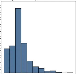
Fig. 3.2: Histogram of the mixture model

Let’s illustrate this method. By examining the following mixture distributionY ∼0.3U(0,20) +

0.7 exp(σ=15,µ =20), a sample of size 1000 is generated from this mixture. The histogram of the

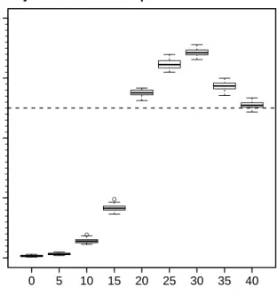
data is presented in Figure 3.2. Figure 3.3 shows the output of the Bayesian method when applied to

the generated sample at an array of thresholds(0,5,10, ...,40). Just as carried out when considering the

MEF, we set the threshold at 20. The output clearly shows thatu=20 is the lowest threshold such that the

resulting predictivep-value is closer to 0.5. This method will be used in subsequent chapters to ascertain

● ●

u

Predictiv

e p−v

alue

Bayesian method example

0.0 0.2 0.4 0.6 0.8 0 5 10 15 20 25 30 35 40

Fig. 3.3: Plotted predictivep-values from a mixture distribution for an array of ordered thresholds

3.5

The Peaks Over Threshold Methodology

Depending on the type of the observations, there are specific methods outlined in the literature to handle extreme value data, see e.g. [Pickands, 1975] and [Coles, 2001]. In this section we focus on the

Peaks Over Thresholdmethodology, which uses the exceedancesxiu,i=1, ...,nthat fall beyond a high

valueuto fit a generalized Pareto distribution to the excessesxiu−ufor some given samplex1,x2, ...,xN,

N is the sample size, while n is the number of exceedances. Most frequently, the parameters of the

GPD are estimated by maximum likelihood (ML), namely due to the favorable properties of this method, [Casella and Berger, 2002].

3.5.1 Maximum Likelihood Estimation

Suppose that the values z₁,z₂, ...,zn are the excesses for a given threshold u. We can obtain the

likelihood function for the generalized Pareto distribution from (3.2). Let Z have a GPD distribution

with shape parameterkand scale parameterσ then fork∈R\ {0}

dF(z) dz = 1 σ 1−kz σ 1_k−1 , (3.11) thus L(σ,k;z1,z2, ...,zn) = 1 σn n

∏

Applying the natural logarithm to both sides, we obtain

l(σ,k;z1,z2, ...,zn) =ln 1 σn + n

∑

∑

so that(1−k zi/σ)>0 fori=1, ...,n. In the case wherek=0 we can derive the likelihood function as follows dF(z) dz = 1 σe −z σ, hence L(σ;z1,z2, ...,zn) = 1 σn n

∏

applying the natural logarithm to both sides, we obtain

l(σ;z1,z2, ...,zn) =−nln(σ)− 1 σ n

∑

The usual analytical procedure for the maximization of the log-likelihood function does not provide

separate expressions for the estimates ofkandσ in the case where the former differs from 0. Hence, a

numerical technique is required, see [Grimshaw, 1993].

There is an abundance of literature on estimating the parameters of the GPD by other methods be-sides ML, such as the following: [Castillo and Hadi, 1997], [de Zea Bermudez and Kotz, 2010a] and [de Zea Bermudez and Kotz, 2010b]. Maximization of the previous functions with respect to the

parame-ters(σ,k)produces maximum likelihood estimators(σˆ,kˆ), which have been shown to be asymptotically

normal and asymptotically efficient under certain conditions of regularity. These conditions are needed,

since whenk>0, the support of the generalized Pareto distribution is dependent on its parameters.

Fork=0, the GPD is reduced to the exponential distribution. Simple derivation methods are

suffici-ent to obtain maximum likelihood estimators in this case. LetZ∼Exp(σ)andz1,z2, ...,zn be a sample

derived fromZ. Then, by maximizing (3.14), we obtain

dl(σ;z1,z2, ...,zn) dσ =0, −n σ+ 1 σ2 n

∑

∑

then, the estimator of sigma is ˆσ=Z.

Hence, the mean is a natural estimator ofσ. It is easy to derive confidence intervals forσ by the

asymptotic properties of ML estimators.

Fork6=0, [Castillo and Hadi, 1997] outlines an algorithm to compute statistically efficient estimators

fork andσ that rely only on two distinctive order statistics in a random sample. The authors also lay

methodology out to derive confidence intervals forkandσ using the delta method.

3.5.2 Estimation of Extreme Quantiles

The topic of extreme quantile estimation has been thoroughly studied in the literature, such as [Coles, 2001], [Grimshaw, 1993] and [Hosking and Wallis, 1987]. In this chapter, we summarize the method described in [Coles, 2001] for extreme quantile estimation. Consider that the generalized Pareto

distribution (for some unknown parameters k6=0 andσ) is suited to model the excessesx−uover a

P(X>x|X>u) = 1−k x−u σ 1_k , x>u, (3.16) also P(X>x|X>u) =P(X>x,X>u) P(X>u) ⇔P(X>x|X>u) =P(X>x) P(X >u) ⇔P(X>x) =P(X>x|X>u)×P(X >u), thus P(X>x) = 1−k x−u σ 1_k ×P(X >u).

Letτu=P(X>u). The extreme quantile, which is the valuexpsuch thatP(X>xp) =pfor a very small

p, is obtained as follows: 1−k xp−u σ 1_k ×τu=p, ⇔1−k xp−u σ = p τu k , ⇔xp= σ k 1− p τu k +u, (3.17)

where it is necessary that p is a probability close to 0 to ensure that xp>u. For k=0, we obtain xp

applying a similar procedure:

1−(1−e−x−σu) =

P(X>x)

P(X>u),

P(X>x) =e−x−σu×_τu, _τu=P(X>u),

then the extreme quantile with probability 1−pis obtained as follows:

τue− xp−u σ =p, hence xp=σln τu p +u. (3.18)

Note that in both cases we are estimating the(1−p)th quantile, for a very small probabilityp.

Extreme quantile estimation is obtained by imputation of the maximum likelihood estimates of the

GPD parameters. An estimate ofτuis also necessary, asτuis the probability that the random variableX

exceeds the thresholdu. An obvious estimator ofτuis

ˆ

τu=

M

n,

whereMis the amount of order statistics that exceeduandnis the sample size. The number of order

statistics exceeding uhas a binomial distribution, Bin(n,τu), where ˆτu is also the maximum likelihood

estimate ofτu. Therefore, the uncertainty ofτushould also be taken into account.

In the case wherek6=0, in order to calculate confidence intervals for the quantiles, it is necessary to

Mhas distribution Bin(n,τu) and let ˆτu= M_n, whereM is the number of upper order statistics that

exceedu. We can derive the variance of ˆτuas follows:

var M n = 1 n2var(M) = 1 n2[nτu(1−τu)] = 1 n[τu(1−τu)]

The variance-covariance matrix of(σˆ,kˆ,τˆu)is given by

V=   1 n[τu(1−τu)] 0 0 0 v11 v12 0 v21 v22  ,

where vi j are the terms of the variance-covariance matrix of(σˆ,kˆ). These are difficult to obtain. In

[Castillo and Hadi, 1997], the authors outline an algorithm to obtain efficient estimators forσandk, and

also calculate their variance-covariance matrix.

Finally, the standard error for ˆxpcan be obtained via the delta method where the gradient vector of

xpis as follows: ∇xp=    ∂xp ∂ τu ∂xp ∂ σ ∂xp ∂k   =   σpkτu−(k+1) k−1(1−(p/τu)k) −σk−2(1−(p/τu)k)−σk−1(p/τu)kln(p/τu)  

Thus, by the delta method, we obtain

var(xˆp)≈∇xTpV∇xp.

Chapters 4 and 5 present a summary of the delta method and an introduction to Bayesian statis-tics, respectively. These chapters were created so the reader could follow the implementation of both methodologies throughout this dissertation. Those who are acquainted with these domains can forgo the reading of the chapters mentioned above.

4

|

Basics of Bayesian Statistics

In this chapter we present the fundamentals of Bayesian statistics. The objective is to produce a brief account of Bayesian methodologies so the reader can properly interpret the method presented in chapter 3.

The classical statistics approach consists in obtaining a samplex1,x2, ...,xn produced by a random

variableX. X has unknown distribution familyQ_θ and unknown fixed parameter vectorθ. The aim is

to find a suitable model forX and, thus, estimateθ generally via maximum likelihood. Inference on the

parameters is performed by calculating point estimation, confidence intervals and hypothesis testing for

θ.

In this setting, the data is considered to be obtained through a random process, wherex1,x2, ...,xnis

a realization of the seriesX1,X2, ...,Xn, andXi(i=1, ..,n) andX have common distribution. Hypothesis

testing is carried out by considering a null hypothesisH0and a test statisticT following some sampling

distribution. We then calculate the probability that underH₀the test statistic produces a value as extreme

or more extreme than the one calculated from the observed data. This probability is called thep-value. If

the p-value is very low (close to 0), we reject the null hypothesis at some significance level. This means

that our choice is not only based on the observed data, but also on data that was not observed. In this

scope, it is incorrect to consider thep-value a true probabilistic measure of the likelihood ofH0, because

the distribution parameters on whichH0depends are fixed quantities. We will show that in the Bayesian

setting it is possible to obtain such measures.

The Bayesian layout consists in choosing a model, f(x|θ), for the observed data and a model forθ,

π(θ). The latter is termed prior probability distribution, meaning the distribution ofθ before the data is

observed. We then construct the posterior distribution ofθ,π(θ|x), using Bayes’ theorem. We can then

derive credible regions forθ. These can be interpreted as true probabilistic measures of the likelihood of

theθbeing contained in such regions. Using the posterior, distribution we can derive the distribution of

future observations, termed the posterior predictive distribution. Hypothesis testing is performed via the Bayes’ factor where we compute the chances of two distinct hypotheses.

The Bayesian framework offers the advantage of combining known information about the parameter with observed data. This known information about the parameter is incorporated via the prior distribu-tion. High variance prior distributions can be considered when no prior knowledge about the parameter is available, i.e., vague or non-informative prior distributions. A major advantage of Bayesian analysis is that the posterior distribution can be updated as new data becomes accessible, which makes this a great methodology for processing data which becomes available sequentially. This way, a model can be

updated as new data is collected. As the(i+1)th dataset becomes available, theith posterior becomes

the(i+1)th prior.

The Bayesian sphere does not rely on asymptotic theory. There is no distinction in the procedure for small or large samples. Informative priors become more important when the available data is scarce.

The freedom in choosing the prior distribution for the model’s parameters might be a downside if not addressed correctly. The posterior distributions are influenced by the selected prior. Hence, if no information is available, one should choose a prior that yields the least amount of information.

This methodology comes with huge computational burden due to the usual numerical costs of cal-culating the posterior distribution. As an example, the Bayesian method for threshold selection using measures of surprise required one to two hours of computational effort to process information about

8174 individuals, using an i7 intel core processor.

4.1

Bayes’ Theorem

In this section we present the Bayes’ theorem and how it is derived in the discrete and continuous

case. Let A and B be two events (events are sets with measureP). The conditional probability of A given

B is given by

P(A|B) =P(A∩B)

P(B) , P(B)>0.

Using the law of total probability, we can writeP(B) =P(A∩B) +P(A¯∩B). Thus

P(A|B) = P(B|A)P(A)

P(A∩B) +P(A¯∩B) =

P(B|A)P(A)

P(B|A)P(A) +P(B|A¯)P(A¯).

4.1.1 The Discrete Case

LetX be a random variable wherex is the observed data (of size n) and f(x|θ) is an appropriate

model for it. We considerπ(θ)the prior distribution ofθ which is the parameter vector with a discrete

support. θcan only take values in{θ1,θ1, ...,θm}. Using Bayes’ theorem, we can write

π(θi|x) =

f(x|θi)π(θi)

∑mj=1f(x|θj)π(θj)

,i=1, ...,m,

whereπ(θi|x)is the conditional distribution ofθigivenx, also known as the posterior distribution ofθi.

4.1.2 The Continuous Case

Without loss of generality, we consider the case whereθ is an unidimensional parameter and has a

continuous distributionπ(θ)with support

Θ={θ:π(θ)>0},

and letX be a random variable with density function f(x|θ) that belongs to the family of distributions

ϒ={f(x|θ):θ ∈Θ}. Now, let(x1,x2, ...,xn) be a realization of the series of i.i.d. random variables

(X1,X2, ...,Xn)that have common distribution withX. Then, using Bayes’ theorem, we can write

π(θ|x1,x2, ...,xn) = f(x1,x2, ...,xn|θ)π(θ) R Θf(x1,x2, ...,xn|θ)π(θ)dθ ,θ∈Θ ⇔π(θ|x1,x2, ...,xn) = ∏ni=1f(xi|θ)π(θ) R Θ∏ n i=1f(xi|θ)π(θ)dθ ,θ∈Θ.

LetL(θ|x1,x2, ...,xn) =∏ni=1f(xi|θ)be the likelihood function of the observed data. We can write the previous relation as π(θ|x1,x2, ...,xn)∝L(θ|x1,x2, ...,xn)×π(θ), since Eθ(L(θ|x1,x2, ...,xn)) = Z Θ n

∏

4.2

Predictive Posterior Distribution

Irrespectively of the approach which is used (classical or bayesian), one of the purposes of data modeling is the prediction of future observations. In a Bayesian framework, the prediction of future observations is performed by means of the predictive distribution. The distribution of a future observation

yis given by

m(y|x) =

Z

Θ

f(y|θ)π(θ|x)dθ,

wherex= (x1,x2, ...,xn)is the observed data.π(θ|x)represents the posterior distribution ofθand f(y|θ)

represents the model for the future datay. In the formula written above, yandx are considered to be

conditionally independent givenθ. This distribution is notθ-dependent, since the parameter is integrated

out.

4.3

Bayes’ Factor

Similar to classical hypothesis testing, in the Bayesian sphere, we consider a null hypothesis H₀:

θ∈Θ. The key difference is thatθhas known prior and posterior distributions, unlike classical statistics,

where the parameters are fixed. Hence, it is possible to answer the question: what is the probability of

H₀? This question can be further divided. What is the probability of H₀ a priori, i.e., before seeing

the data? What is the probability ofH0 a posteriori? What is the probability ofH0 against some other

hypothesisH1? In this section we present a methodology that will produce answers to these questions.

Letθ∈Θbe the parameter we intend to infer on. Letπ(θ)andπ(θ|x)be the prior and the posterior

distribution ofθ, respectively. We consider the null hypothesisH0: θ∈Θ0 vs H1: θ∈Θ0. The prior

odds ofH0againstH1is defined as

O(H₀,H₁) =P(H0)

P(H1)

.

The posterior odds ofH0againstH1can be obtained similarly

O(H0,H1|x) =

P(H0|x)

P(H1|x)

.

Considering thatθ has a continuous distribution, then

O(H0,H1) = R Θ0π(θ)dθ R Θ0π(θ)dθ , and O(H₀,H₁|x) = R Θ0π(θ|x)dθ R Θ0π(θ|x)dθ .

Low values (close to 0) ofO(H0,H1)suggest thatH1is more likely thanH0, while the converse suggests

thatH₀is more likely thanH₁. The interpretation of the posterior odds is the same. Bayes’ factor ofH₀

againstH1is given by

B=O(H0,H1|x)

O(H0,H1)

.

It has similar interpretation to the prior and posterior odds. High values ofBpoint towardsH₀while low

values (close to 0) favorH1. B measures to what extent the strength of the evidence changed our belief

inH0againstH1.

Table 4.1: Bayes’ factor output interpretation by [Kass and Raftery, 1995]

B Strength of the evidence in favor ofH0

1 to 3 not worth more than a bare mention

3 to 20 positive

20 to 150 strong

>150 very strong

4.4

Predictive

p

-values

Traditionalp-values can be interpreted as the probability of obtaining test statistic values as large as

or greater than the one observed under the null hypothesis, thus calculating some probability area of the

distribution’s tail. Something similar can be obtained in the Bayesian framework. The predictivep-value

can be computed using the following condition

pm=P(T(y)≥T(x)|x,H0), H0:θ∈Θ0,

where yare future observations, i.e., data generated from the predictive posterior distribution, xis the

observed data andT a given test statistic. IfT is free of nuisance parameters, then pm can be

calcula-ted. [Meng, 1994] addresses the topic of calculating the predictive p-value whenT includes nuisance

parameters.

We now outline a bootstrap procedure to compute an estimate of the predictivep-value:

1. Calculate the predictive posterior distributionm(y|x).

2. Generateyi=yi1,yi2, ...,yim,i=1, ...,n, fromm(y|x).

3. Choose a test statisticT.

4. ComputeT for eachyiand for the observed datax.

5. The predictivep-value is given as: pm=k_n, wherek=#{T(yi)>T(x),i=1, ...,n}.

5

|

The Delta Method

Given a random variableX, it is sometimes necessary to obtain the distribution of a function ofX.

For example, the transformation of an estimator ˆθ byg(.), whereg(.)might be a quantile function.

De-pending on the selected transformation functiong(.), direct estimation of the desired distribution might

range from trivial to impossible. Hence, we must rely on approximation methods to obtain the intended distribution for the latter case. The delta method provides an algorithm to obtain such approximation

under certain conditions of regularity for X andg(.).

Theorem 5.0.1 (Taylor’s series with remainder) Let f ∈Cn+1with domain that contains a. The Taylor formula for every x in this interval is given by

f(x) = n

∑

For interested readers, [Apostol, 1967] presents a demonstration of this theorem. Regarding the remainder, it can be shown that

lim x→a

Rn(x)

(x−a)n =0. (5.3)

Hence, we can approximate f by a polynomial functionPn(x)with degreen. Asx→a, this

approxima-tion has an error of smaller order than(x−a)n.

We will use aTaylor seriesof first order as a tool to obtain an approximation ofg(.). We assume that

Znis a sequence of random variables such that

√

n[Zn−θ]

D

−→N(0,σ2),σ>0. (5.4)

The goal is to obtain the distribution of g(Zn). Let g(.)∈C1, such that g0(z)6=0. We consider the

following first order Taylor expansion ofg(.)aroundθ.

g(Zn)≈g(θ) +g0(θ)(Zn−θ). (5.5)

Note that for this approximation we assume that the remainderR1(Zn)is 0, the reason being that we are

computing the Taylor series in θ, the assumed mean value ofZn. Hence, we infer that as long asn is

large enough,Zn→θin probability. Thus by (5.3),R1(Zn)→0 in probability.

Here we outline how to estimate the expectation and variance ofg(Zn). Taking expectation on both

sides of (5.3), we obtain

E[g(Zn)]≈E[g(θ) +g0(θ)(Zn−θ)]

=g(θ) +E[g0(θ)((Zn−θ)]

=g(θ) +g0(θ)E[(Zn−θ)] =g(θ).

Similarly, we apply the variance to both sides of (5.3). Consequently, Var[g(Zn)]≈Var[g(θ) +g0(θ)(Zn−θ)] =Var[g0(θ)(Zn−θ)] =g0(θ)2Var[(Zn−θ)] =g0(θ)2σ2. (5.7)

Let’s "play"with the expression√n[g(Zn)−g(θ)]. Replacingg(Zn)by its Taylor first order

approxi-mation, we obtain _√ n[g(θ) +g0(θ)(Zn−θ)−g(θ)] = √ n[g0(θ)(Zn−θ)] =g0(θ) √ n[Zn−θ]. (5.8) Hence,√n[g(Zn)−g(θ)]≈g0(θ) √

n[Z−θ]. Using this approximation, we want to obtain the distribution

family for√n[g(Zn)−g(θ)]. LetB=

√ n[Z−θ],B∼N(0,σ2)by construction. Consequently P(g0(θ)B≤b) =P B≤ b g0_(θ) =FB b g0_(θ) ,

whereFB(b)is the distribution function ofB. We now calculate the derivative

F_B0 b g0(θ) = fB b g0(θ) d d b b g0(θ) = fB b g0(θ) 1 g0(θ), where fB(b) = 1 σ √ 2π e− b 2 2σ2. Hence F_B0 b g0(θ) = 1 σ √ 2π e− b g0(θ) 2 2σ2 1 g0(θ) = 1 g0(θ)σ √ 2π e− b2 2σ2g0(θ)2_,

which corresponds to the density function of Normal distribution N(0,σ2g0(θ)2). Thus,g0(θ)√n[Z−

θ]≈N(0,σ2g0(θ)2). Since √ n[g(Zn)−g(θ)]≈g0(θ) √ n[Z−θ], we say that √ n[g(Zn)−g(θ)]∼N(0,σ2g0(θ)2).

This methodology is well suited to obtain the distribution of transformations of maximum-likelihood estimators. We will now present the case where we intend to infer on a transformation of a vector of

maximum likelihood estimators. Let ˆθ= (θˆ1,θˆ2, ...,θˆm), the vector of estimators with meansE(θˆi) =θ

such that ˆθ−→D N(0,Σ), whereΣis the variance-covariance matrix of ˆθ. Letg:Rn−→Rwith non null

first order partial derivatives. The Taylor’s first order expansion ofg(.)around ˆθ = (θ1,θ2, ...,θm)is as

follows:

g(θˆ) =g(θ) +∇Tg(θ)(θˆ−θ), (5.9)

where ∇Tg(θ) is the gradient vector of g(.), ∇Tg(θ) = [_{∂ θ}∂g

1, ∂g

∂ θ2, ..., ∂g

∂ θm].Taking expectations on both

sides, we obtain

E[g(θˆ)] =E[g(θ) +∇Tg(θ)(θˆ−θ)]

=g(θ) +∇Tg(θ)(E[θˆ]−θ)

=g(θ).

(5.10)

We now apply the variance to both sides of (5.9), hence obtaining

Var[g(θˆ)] =Var[g(θ) +∇Tg(θ)(θˆ−θ)],

=Var[∇Tg(θ)(θˆ−θ)]

=∇Tg(θ)Σ∇g(θ).

Similar to the univariate case, we can show that√n[g(θˆ)−g(θ)]−→D N(0,∇Tg(θ)Σ∇g(θ)).

Confi-dence intervals for the univariate and multivariate cases can be constructed using the following formulas:

IC1−α=g(θ ∗ )±z₁₋α 2 × r g0(θ∗)2σ2 n , (5.12) IC1−α=g(θ ∗_)± z₁−α 2 × r ∇Tg(θ∗)Σ∇g(θ∗) n , (5.13) where z₁₋α

2 is the quantile with probability 1−

α

2 from a standardized normal distribution, α is the

6

|

Descriptive Analysis of the Biometric

Variables Recorded in Portuguese

Vo-luntary Pharmacy Attendees

6.1

Introduction

Hypertension, also known as high blood pressure, is described as an abnormal pressure on the blood vessels caused by blood flow. As blood is pumped through the body, the blood vessels are impacted by this flow, thus creating blood pressure and blood vessel tension. The higher the tension, the more strength the heart needs in order to pump the blood. Diagnosing hypertension is done by measuring two blood pressure markers. Systolic blood pressure is the tension measured by the compliance of the blood vessels to the blood flow during a heartbeat. Diastolic blood pressure is the tension measured between heartbeats.

According to the World Health Organization (WHO), hypertension is a global public health issue. It is highly associated with incidents of heart disease, stroke, kidney failure, premature mortality and disability. In Portugal medical practitioners state that half of the adults of age 40 and higher suffer from hypertension and one third has not been diagnosed. This is due to most of the early onset symptoms of the disease being very mild. It is also the risk factor most associated with the leading death causes in the country.

Hypertension has been linked to unhealthy diets, sedentary lifestyle, drug abuse and tobacco use, see [Schröder et al., 2003] and [Wakabayashi, 2004]. The former studies the relationship between diet, body mass index, cholesterol, leisure-time physical activity and diet on the Mediterranean Southern-Europe population, while the latter studies the relationship of the body mass index with blood pressure and serum cholesterol concentrations at different ages. See also [Hajar, 2016], where the author outlines the history of the study of risks associated with hypertension.

With the goal of addressing this public health issue, the Portuguese National Association of Pharma-cies developed a campaign in 2005 through their Department of Pharmaceutical Care to study the risk factors associated with the leading death causes in the country.

In the following section, we will descriptively analyze several biometric variables as a factor of some other measures of interest (on the individuals who suffer from isolated systolic hypertension), such as the relation between systolic blood pressure and age, tobacco consumption, body mass index and gender.

In the next two chapters, we will apply the aforementionedPeaks Over Thresholdmethodology to the

individuals who suffer from isolated systolic hypertension, which are characterized by havingdiastolic

blood pressure <90 mmHg and systolic pressure ≥140 mmHg. The classification categories in terms of blood pressure conditions are presented in table 6.1 (guidelines of the Portuguese Cardiology

Association). The goal is to fit a generalized Pareto distribution to the excesses above a high thresholdu

for each Portuguese district, and subsequently estimate tail probabilities and extreme quantiles. With this study, we hope to answer questions about the condition of the most extreme isolated systolic hypertension cases for each district.