Point Sensitivity for Radial Visualization under Dimensional Anchor Motion

Point Sensitivity for Radial Visualization under Dimensional

Anchor Motion

A. Russell University of Massachusetts USA 01854, Lowell, MA arussell@ cs.uml.edu F. Kamayou University of Massachusetts USA 01854, Lowell, MA fkamayou@ cs.uml.edu R. Marceau University of Massachusetts USA 01854, Lowell, MA rmarceau@ cs.uml.edu K. Daniels University of Massachusetts USA 01854, Lowell, MA kdaniels@ cs.uml.edu G. Grinstein University of Massachusetts USA 01854, Lowell, MA grinstein@ cs.uml.edu

ABSTRACT

This paper extends prior work withnormalized radial visualizations(NRVs) that includes the RadViz mapping onto the two-dimensional unit disk. Here we examine point sensitivity under varying assumptions about dimensional anchor motion. First, we describe the role of the barycenter of the dimensional anchors as the position where records map to under a NRV when all of their dimensional values are equal. Next, we explore the intuition that data records whose standard deviation across the dimensions is small map close to the barycenter under a NRV; such data records have low mobility. When the dimensional anchors are arranged uniformly on the RadViz circle, our distance formulation provides a preprocessing test that is sufficient for concluding that a record will lay within a circle of radius 1₂ around the barycenter. This test is independent of the ordering of the dimensional anchors on the circle. Then, for RadViz we employ a robotic motion planning analogy which utilizes the Minkowski sum to show that when some of the dimensional anchors’ positions are free to move on the unit circle, then a data record maps inside an annulus, whose center, inner and outer radii are computable. Extending the motion planning analogy, we are able to determine a dimensional anchor configuration which places a data record image point at a chosen position. To illustrate this, the Weave visualization system has been enhanced to include interactive point sensitivity features.

Keywords

Computer Graphics, Radial Visualization, Visual Analytics

1

INTRODUCTION

Radial visualizations, with some variety in con-struction, originated in the 19th _century.

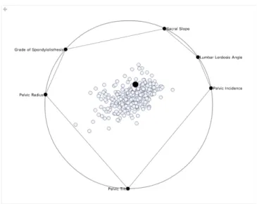
Rad-Viz [HGM+97b] is a 2Dvisualization that displays d dimensional data by arranging labels at points on the circumference of the unit circle. Figure 1 shows an example of a basic RadViz image for a dataset with 14 dimensions. RadViz can be viewed as a partic-ular instance of a Normalized Radial Visualization (NRV) [DGRG12], which describes a transformation in Euclidean space fromEd→Ed′, whered′=2 (see Section 1.1). Each ofndata records are then associated with points on the interior of the circle by way of the RadViz algorithm. The labels located on the unit circle

Permission to make digital or hard copies of all or part of this work for personal or classroom use is granted without fee provided that copies are not made or distributed for profit or commercial advantage and that copies bear this notice and the full citation on the first page. To copy otherwise, or re-publish, to post on servers or to redistribute to lists, requires prior specific permission and/or a fee.

Figure 1: A RadViz image of a 14ddata set [DGRG12]. are called Dimensional Anchors (DAs), one for each of theddimensions.

This paper examines point sensitivity for this type of ra-dial visualization under varying assumptions about di-mensional anchor motion. That is, we observe how a data record’s position in the image space changes as di-mensional anchors move (how sensitive the point is to changes in DA positions). The literature on this topic is scarce. The closest work appears to be Reem’s [Ree11] examination of how the geometric characteristics of

a Voronoi diagram [Aur91] change under small per-turbations of the sites. Yi et al. [YMSJ05] discuss data records moving towards dimensional representa-tives (see Section 1.1).

Our approach begins in Section 2 by highlighting the NRV barycenter (average, center or centroid) of the dimensional anchors as the position where records map to when all of their dimensional values are equal. This can differ from the RadViz unit disk’s center. Records whose standard deviation across the dimensions is small map close to the barycenter, and we derive a bound on this distance that applies to arbitrary dimension of the NRV image space. Such records have low mobility under motion of the dimensional anchors. Next Section 3 uses a motion planning analogy (see Section 1.2) in the RadViz context to show that, when some of the dimensional anchors’ positions are free to move on the unit circle, then a data record maps inside an annulus, whose center and inner and outer radii we provide. The motion planning analogy extends further to allow us to, given any point on a data record’s annulus, reverse-engineer to recover a set of dimensional anchor positions that yield that point. An earlier version of Sections 2 and 3 appears in the PhD thesis [Rus13]. Section 2 extends beyond [Rus13] the bound on barycenter distance to arbitrary dimension of the NRV image space. Section 3 generalizes the annulus center and radius calculation to accommodate moving an arbitrary number of DAs.

These results are beneficial to the visualization analyst who wants to understand the freedom of movement of data record image points under motion of the dimen-sional anchors. For this paper the Weave visualization system [DSFG12] has been enhanced to include inter-active point sensitivity features. Weave is a highly in-teractive open source web-based visualization platform that provides the ability to integrate, analyze, and visu-alize distributed data and databases, and to disseminate the results in a web page. Weave is available on the github public code repository. Section 4 provides con-clusions and offers avenues for future research.

1.1

Normalized Radial Visualization

Early examples of radial visualizations are William Playfair’s pie charts and Florence Nightingale’s polar plots [WGK10]. Draperet al.provide a comprehensive survey of radial visualizations [DLR09]. Diehl et al. empirically evaluate the strengths and weaknesses of radial visualization for a task such as memorizing positions of visual elements, and they suggest that radial visualization, while outperformed in some ways by Cartesian coordinates, can help the user focus on specific data dimensions [DBB10]. Some additional examples of advances in the use of radial visualiza-tions include Circle Segments [AKK96], 2D Star

Coordinates [Kan00], 3D Star Coordinates [SY06], RadViz [HGM+97a], and SphereViz [SDC07]. Yiet al.[YMSJ05] describe a radial visualization that employs “magnets”, which exhibit and attraction force with a point based on the product of the dimension’s value in the data record and the strength of the magnet. In a manner similar to the RadViz DAs, the magnets act upon only a single dimension. The magnets may also be moved and the motion of the particles examined. Unlike RadViz, the magnet may also repel a particle. Tominskiet al.[TA04] describe several different visual-ization methods which take high dimensional data and map it to a 2Dimage space. Although their TimeWheel is oriented toward datasets that have a temporal com-ponent, it may be used for other datasets where an in-dependent variable is chosen as the variable of focus. Once this focus variable is placed in the center, the ordering of the remaining variables poses a difficulty as in RadViz and Parallel Coordinate [ID90] visualiza-tion. Both their MultiComb and spike glyph are sim-ilar, however less sensitive to the arrangement of the non-focal component. This is in contrast with RadViz, where there is no particular component that is the focus of the analysis.

Daniels et al. [DGRG12] establish a number of theoretical properties of radial visualizations as well as rigorously formulate a broader class of Radial Visualizations – the aforementioned NRVs. RadViz is shown there to be a special instance of NRVs. RadViz has been shown in the literature to be useful for multi-dimensional data. For example, DiCaro

et al. [DCFMFM10] use d _≤ 8, Figure 1 shows

d =14, Daniels et al. include a RadViz example from bioinformatics with 6817 genes, each associated with a dimensional anchor, and RadViz is applied in bioinformatics for supervised learning in [KB10]. Other RadViz research includes integration of RadViz with Parallel Coordinates by Bertini et al.[BAS+05], Vectorized RadViz [Sha04, SGM08, Zim11] and using RadViz to visualize time series data [NS11].

Prior to Daniels et al. other authors, such as Nováková [Nov09] and McCarthy et al.[MMH+04], had offered informal observations on properties for-mally stated and proved in Daniels et al.[DGRG12], such as points which lie on a line crosscutting the origin map to a single point in the RadViz plane. McCarthy [MMH+04] states “points with approxi-mately equal dimensional values will lie close to the center.” In this paper we show that thebarycenterof the DAs is actually involved; in McCarthy’s case the barycenter is coincident with the center of the unit disk. The RadViz mapping is analogous to spring forces us-ing Hooke’s Law. Informally we may picture each data image in RadViz as being tethered to multiple springs, one for each dimension, with each of these springs

at-Figure 2: An illustration of RadViz’s spring force anal-ogy [GYLG05].

tached to one of the DAs (see Figure 2). These springs “pull” the data image towards the circumference of the circle. To formulate the mapping [DGRG12], we start with the stretching forces (~F) ofd springs under Hooke’s law for theithdata recordvi. At equilibrium

we have: d−1

∑

j=0 ~ Fj=0= d−1

∑

j=0 vi,j(~Sj−~x) (1)

whereF~j=k~xfor ksome spring constant and k~xk is

the stretched distance. The stretched distance is the dis-tance from the DA to a point in the two-dimensional image space. We substitute forkthe data record’s value for the jthdimension: vi,j. Forxwe substitute the

dis-tance between the DA~Sjon the unit circle and the data

record’s imagexand then solve for~x:

~x=∑ d−1

j=0~Sjvi,j

∑dj=0−1vi,j

. (2)

In two-dimensional RadViz we then have:

xi,1= ∑d_j=0−1cos(θj)vi,j ∑dj=0−1vi,j xi,2= ∑d_j=0−1sin(θj)vi,j ∑dj=0−1vi,j . (3) In the above expressions~Sjis decomposed into its

com-ponents for thexi,1andxi,2position of the DA (respec-tively, in Cartesian coordinates, cos(θj)and sin(θj)).

These expressions are generalizable to higher dimen-sional NRVs [DGRG12]. Thus, RadViz is a spe-cial case of an NRV. Here we list several character-istics of NRVs which were established in Daniels et al.[DGRG12] and are applied in this paper:

1. The scaling transformation η, where for the ith recordviin a data set ofd dimensions,ηiis a

per-spective transformation:

ηi=

1 ∑d_j=0−1vi,j

. (4)

2. Theη transformation projects each data point onto a simplex facet which is the intersection of the pro-jective hyperplane∑jj==0d−1Dj=1 with the positive

orthant. HereDjis a variable for the jthdimension.

3. The η transformation is composed with an affin-ity [FR87, Far02] which takes points from the sim-plex facet to inside the convex hull of the DAs. This does not require the DAs to be cocircular.

4. An NRV maps lines to lines, ellipsoids to ellipsoids, and preserves point ordering and convexity.

Usingηwe can reformulate Eq. 2 as:

~x=ηi d−1

∑

j=0

~Sjvi,j. (5)

DAs need not be on the circle in an NRV, but for some of our RadViz results we assume that they are, as is customary.

1.2

Motion Planning

In Section 3 we demonstrate a link between some con-cepts from robotic motion planning and point sensitiv-ity. O’Rourke [O’R98] explores in depth the motion planning subfield of a so-called “robot arm.” This arm is a succession of fixed length segments with one end in a fixed position referred to as the “shoulder,” where the shoulder is assumed to be at the origin. For anm-link robot arm we label each of themlinks asℓm. Given

m link lengths connected to an arm, the reachability problem asks: “which points in the plane can them-link arm’s outer tip reach?”

O’Rourke relates results attributed to Hopcroft et al. [HJW85] that address this. Hopcroft et al. also prove a theorem which allows us to compute the inner and outer radii of the annulus: “The reacha-bility region for an m-link arm is an origin centered annulus with outer radius ri,O =∑ml=1ℓl and inner

radius ri,I =0 if the longest link length ℓM is less

than or equal to half the total length of the links, and ri,I =ℓM−∑l6=Mℓl otherwise.” The annulus

results rely on the Minkowski sum of two setsB1and

B2, which is defined as the set of pairwise sums of points from each of the two sets. Formally we write B1⊕B2={b1+b2|b1 ∈B1,b2∈B2} [dBvKOS00]. The Minkowski sum is associative [GS93].

A recursive procedure is described by O’Rourke which, when supplied with a point pin the annulus, reverse-engineers angles for the robot arm’s links that allow the arm to reach that point. The base case is one involving 3 links, which can be solved using several cases based

on intersection of a circle with an annulus. At theith level of the recursion the problem is to reach a pointpi.

A circle of radiusℓiis constructed, centered at pi, and

that circle is intersected with the annulus for the first i₋1 links to produce a pointti. A set ofi−1 angles are

determined recursively in order to reachtiand then link

li is added to the result to allow connection oftito pi.

The procedure’s running time is linear in the number of links.

O p

Figure 3: An example of an annular reachability re-gion for a robot arm, with 4 links, shouldered at O, together with a link configuration allowing the arm to reach pointp.

Figure 3 illustrates an example of an annular reacha-bility region for a 4-link robot arm. In Figure 3 the arrangement of 4 links allowing the tip of the arm to reach pointpforms a link configuration.

2

BARYCENTER PROXIMITY

The barycenter (average, center, or centroid)bP of the

DAs is expressed as:

bP=

∑dj=0−1~Sj

d (6)

Figure 4 illustrates the barycenter of a set of di-mensional anchors for the 310 records from the 6-dimensional Vertebral Column dataset [BL13]. Note that the barycenter of the DAs in Figure 4 is not at the unit disk’s center. Data record images that are close to bP are undesirable, partly because they can represent

cancellation of opposing DA contributions. In addition, we show that the barycenter is the place where records of all equal dimensional values map to. Starting from Eq. 3 we have: xi,1= ∑dj=0−1cos(θj)v0 ∑dj=0−1v0 =∑ d₋1 j=0cos(θj) d (7) and, similarly, xi,2= ∑dj=0−1sin(θj)v0 ∑dj=0−1v0 =∑ d₋1 j=0sin(θj) d (8)

Figure 4: The barycenter and convex hull for an ar-rangement of DAs. Data points represent the 310 records from the 6d Vertebral Column dataset [BL13] shown in Weave [DSFG12].

This yields Eq. 6. We note that this result extends to all NRV’s. Furthermore, it does not require the DAs to be cocircular. The impact is that, regardless of where the DAs are placed, such recordsalwayslie at the barycen-ter of the DAs.

We observe that having records of all equal dimensional values map to the barycenter implies a corollary to Lemma 2.1 of Danielset al.[DGRG12]. That lemma, which applies to NRV transformations, involves the

η mapping and is summarized in item 2 in our Sec-tion 1.1. The corollary is that the linex1=x2=···=xd,

which is perpendicular to the simplex facet associated withη, maps under theη transformation to the center of the simplex facet, which then maps, under the affin-ity which takes the simplex facet into the NRV image space, to the barycenterbPof the dimensional anchors.

Thus, the linex1=x2=···=xdmaps to the barycenter.

2.1

Upper Bound on Distance from

Barycenter

Here we relate a data image’s distance in thed′ -dim-ensional image space from the NRV barycenter bP to

the standard deviation of the data values across thed dimensions in the original data space. The 2DRadViz context is the special case in whichd′=2. This devel-opment does not assume that the dimensional anchors are uniformly placed on a circle, nor must they even be cocircular.

First we formulate dimensional value vi,j for data

record vi in the data space in terms of the standard

deviationσiof its dimensional component values, and

the record’s mean ¯vi=

∑dj=0−1vi,j

σi= v u u t 1 d d−1

∑

j=0 (vi,j−v¯i)2 (9) (vi,j−v¯i)2=σi2d− d₋1

∑

l6=j (vi,l−v¯i)2 (10) vi,j= v u u tσ_i2d− d₋1

∑

l6=j (vi,l−v¯i)2 + v¯i. (11)

Let us call the square root termγ. So, the NRV map-ping, as expressed in Eq. 5 usingηi from Eq. 4, now

looks like this (for the kth component in the image space): xi,k = ηi(S0k(γ0+v¯i) +···+Sd−1k(γd−1+v¯i)) = ηi d−1

∑

j=0 Sjk(γj+v¯i) ! . (12) We notice that ¯vi= ∑d_j=−01vi,j d = η−1 i d . So we may rewrite this as: xi,k=ηi d−1

∑

j=0 Sjk(γj+ η−1 i d ) ! . (13) If we cancel theη′

isand group terms conveniently we

have: xi,k=bP,k+ηi d−1

∑

j=0 Sjkγj ! . (14) wherebP,kis thekthcomponent of the barycenter. Thus,

the distance of, for example, the kth component of the NRV projected point to the kth component of the barycenter of the DAs is:

xi,k−bP,k=bP,k+ηi d−1

∑

j=0 Sjkγj ! −bP,k (15) or just: ηi d−1

∑

j=0 Sjkγj ! . (16)

If we make some substitutions to remove the γ terms we have: ηi d−1

∑

j=0 Sjk(vi,j−v¯i) ! . (17)

The Euclidean distance, in the image space, from the barycenter is: Dist(xi,bP)=ηi v u u t d′

∑

k=1 d−1

∑

j=0 Sjk(vi,j−v¯i) !2 . (18)

Finally, if we holdηi(vi,j−v¯i)≤ d√1ρ, whereρ is an arbitrary constant, we then have:

Dist(xi,bP)≤ s 1 √_ρ 2 + 1 √_ρ 2 (19) Dist(xi,bP)≤ s 2 ρ. (20)

Thus, we are able to identify a circular region, centered at bP with radius Dist(xi,bP)≤

q

2

ρ, in which points satisfying this condition must lay.

In the case whenσi=0 any of thevi,j are equal to ¯vi

and so the total distance frombPis 0, as we would

ex-pect from earlier in this section. The alternate way of showing this result using the standard deviation assists in appealing to our intuition concerning the relationship between the data record values and the point locations within the circle.

In RadViz, as σi increases the distance from bP

in-creases to a maximum of 2, the maximum possible in the unit circle. The maximum distance of 2 may be closely approached in a case such as the following ex-ample: givend DAs place all but one at(0,1). Place the one remaining DA at(0,−1). We are then able to see that the distance may be calculated as 1+(d₋2)/d. For the 100ddata record<1,0,0, . . . ,0>with D0 the DA at(0,−1)we find that we have a distance of 1.98. The restriction of points to lay within a circle of ra-diusq_ρ2 centered atbPhas particular significance for

RadViz with uniform placement of DAs. Specifically, if ρ=8 points will then lay within a circle of radius

1

2. Points in that region are of limited usefulness to the user due to, among other factors, the cancellation of forces from opposing DAs. The user would have difficulty assessing which DAs are most influential for points in this region. In the case where we uniformly place DAs on the unit circle we are able to identify, without completing the RadViz transformation, which points are restricted to lay within this region.

3

CIRCULAR DIMENSIONAL

AN-CHOR MOTION

Here we examine the effects on a data image’s posi-tion of dimensional anchor moposi-tion. We assume that

DAs are cocircular and move in circular paths along the common RadViz circle. Section 3.1 allows one DA to move, which moves a data image in a corresponding circle. Section 3.2 moves multiple DAs. This creates an annular region, as in motion planning for a “shoulder-based” multi-link robot arm (Section 1.2). Reverse-engineering a configuration of DA angles for a given position on an annulus is covered in Section 3.3.

3.1

Moving One Dimensional Anchor

Without loss of generality let us move the 0th_{DA in a}

360◦arc, and we solve for recordvi’s image~x:

vi,0(S~0−~x) +···+vi,d−1(S~d−1−~x) =0 (21) ~x= ηi d−1

∑

j=1 ~ Sjvi,j ! +ηiS~0vi,0. (22)

So, by moving any one DA the movement of the point will trace a circular path with center

ηi∑dj=1−1cosθjvi,j,ηi∑dj=1−1sinθjvi,j

and radiusηivi,0. This effect can be seen in Figure 5. Note that the point circle’s center location is determined only by the data record values and DAs that are fixed in position and that the point circle’s radius is determined by the data record values associated with DAs that are moving.

Figure 5: The circular path traced by the single high-lighted point (indicated by the arrow) when the DA for Lumbar Lordosis Angle is moved around the circle. Data points represent records from the Vertebral Col-umn dataset [BL13] shown in Weave [DSFG12]. Cen-ter =(−0.20,0.18)and radius = 0.27.

3.2

Moving Multiple Dimensional

An-chors

To examine the effects of moving multiple DAs we will consider (again, without loss of generality) the case of moving the 0thand 1stDAs in a 360◦arc. The two DAs move independently of each other. In Section 3.1 we

saw that moving any one DA in a 360◦arc results in the data point tracing a circular path. In this case of multi-ple DAs we then have a composition of circular paths. This composition of circular paths may be expressed using the Minkowski sum defined in Section 1.2. As shown in Figure 6 the result of varying more than one DA results in any one data image forming an annulus. In what follows we derive the center and inner and outer radii of the annulus.

Figure 6: The annular path traced by the single high-lighted point (indicated by the arrow) when the DAs for Pelvic Incidence and Pelvic Tilt are moved around the circle. Data points represent records from the Vertebral Column dataset [BL13] shown in Weave [DSFG12]. Center = (−0.14,0.36) and inner radius = 0.14 and outer radius=0.20.

First, returning to our DAs we have:

~x= ηi d₋1

∑

j=2 ~ Sjvi,j ! +ηiS~0vi,0⊕ηiS~1vi,1 . (23) Since the Minkowski sum is associative, varying addi-tional DAs follows similarly. For example, varying a third DA, say, the 2nd one, would be expressed as:

~x = ηi d₋1

∑

j=3 ~ Sjvi,j ! (24) + ηi~S0vi,0⊕ηiS~1vi,1 ⊕ηiS~2vi,2 . See Figure 7 for an example.

For a given data record value, the center of the annu-lus is completely determined by the fixed dimensional anchors (Eq. 26). In general, ifT is a set ofm+1 di-mensional index values for which DAs are varying and Tjis the jthindex inT, then the annulus is:

~x=ci,T+ m

M

l=0

where the center of the annulus is given by ci,T=ηi d−1

∑

j=0,Tj∈/T ~ Sjvi,j. (26)

To obtain its inner and outer radii we use the analogy from robot motion planning summarized in Section 1.2. In our case the robot arm will not necessarily have its shoulder at the origin but this does not affect our appli-cation of this theorem; our shoulder is at the center of the annulus.

For data recordvi, we interpret the radius of each

circu-lar path traced when varying any one DA as the length of any linkℓ. Thus, when varying the 0th_{DA for record}

vi, ℓ0=ηivi,0 and, in general, ℓl =ηivi,l. The outer

radius is therefore: ri,T,O= Tm

∑

l=T0 ℓl= Tm

∑

l=T0 ηivi,l (27)

The inner radius ri,T,I depends, as indicated in

Sec-tion 1.2, on the relative link lengths. Again, letℓM be

the maximum link length for the moving DAs. If this is at most half of the total link lengths, thenri,T,I=0.

Otherwise: ri,T,I=ℓM−

∑

l∈T,l6=M ℓl=ℓM−

∑

l∈T,l6=M ηivi,l. (28)

Since these radii all have ηi as a common factor, the

reach of these links can be seen, then, to be directly proportional to the value vi,j of the record for

dimen-sion j. From this we note that our ability to reposition a data image also is directly dependent onvi,j. The result

of the center, link lengths, inner and outer radii calcula-tions, according to the above, is illustrated in Figure 7 for the case where D0, D1 and D2 are moving.

The outer radius of the annulus associated with a partic-ular data record point is dependent upon the data record value for the dimensions for which the DAs are mobile. It is independent of the location of the fixed DAs or the value of the point’s coordinate in the dimensions which correspond to the fixed DAs. Figure 8 illustrates this by altering the size of the point in the RadViz visualization in proportion to the outer radius of the point’s annulus. This feature provides a use case for the visualization analyst to further explore data relationships by showing the relative mobility of the records.

3.3

Reverse-Engineering Dimensional

Anchor Configuration

Section 3.2 allows us to solve the following problem. Given a point pdetermine if there are DA positions al-lowing a data image to lie atp. This is accomplished by constructing the annulusAand then testing ifpis inA.

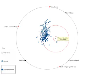
Figure 7: The annular path traced by the single high-lighted point (indicated by the yellow text box) when the DAs for Lumbar Lordosis Angle, Pelvic Radius, and Grade of Spondyloisthesis are moved around the circle. Data points represent records from the Vertebral Column dataset [BL13] shown in Weave [DSFG12]. Center = (0.23,−0.04) and inner radius = 0.07 and outer radius=0.43.

Figure 8: The size of the point varies with the outer ra-dius of the annulus. The annulus outer rara-dius for the selected anchors (in red), is used for setting point size. Points closer to Pelvic Radius and Grade of Spondy-lolisthesis are larger, indicating a stronger expression for these anchors.

Ifpis inA, a natural next question is: can we find a set of DA positions producingp? This reverse-engineering task is addressed here. Again, we use a motion planning analogy; this is the one from Section 1.2 which uses a recursive approach.

The algorithm described by O’Rourke [O’R98] (sum-marized in Section 1.2) is formulated in a recursive fashion. Since our goal is a high-dimensional visual-ization, from a practical point of view we need to avoid recursion stack depth overhead. Our prototype imple-mentation of the algorithm written in Perl uses an it-erative interpretation of the recursive algorithm which

takes into account the properties of our annuli and that our “links" are DAs.

Our iterative algorithm receives as input the data record array, the target point, and an array which contains the indices of the fixed DAs. We start with creating a circle centered at the final target point and an annulus com-posed of the remaining moving dimensions. At each iteration we perform the same intersecting of the circle and annulus as in the recursive algorithm. We select one point from the points of intersection as the target point for the next iteration. As each moving DA is placed we compose a new annulus with the remaining DAs. As with the recursive procedure we conclude when two DAs remain and the annulus problem has reached our base case of intersecting two circles (this is in contrast to O’Rourke’s base case mentioned in Section 1). Fig-ure 3 in Section 1 illustrates an example of a robot arm link configuration.

As an illustration of another use case, the data ana-lyst has moved the point in Figure 7 to a new location (within the annulus). A new configuration for the mov-ing DAs has been calculated and all of the points in the RadViz image have been placed with the new DA con-figuration. The result of moving this point, as it appears in Weave, may be seen in Figure 9.

Figure 9: In comparison with Figure 7, the indicated point was moved to a different location on the annulus and a new configuration of the moving the DAs was calculated.

4

CONCLUSION

This paper contributes to the understanding of point sensitivity in NRVs, that is, where and how data record images move under DA motion. We have shown that the barycenter of the DAs in a NRV is important be-cause data records whose dimensional values are all equal map to the barycenter, regardless of the posi-tions of the DAs. (Note that the barycenter changes

when the DA positions change.) Our bound on the dis-tance from a data record’s image to the barycenter can form the basis for a preprocessing step for exploration in radial visualization where the DAs are placed uni-formly. We have presented a correspondence between robot arm motion in the 2Dplane and circular motion of DAs. This confines a data record’s image to an an-nulus, whose center and inner and outer radii we pro-vide. Given a point in an annulus we also show how to recover an associated DA configuration. This can po-tentially be extended to solve the following problem: givenkpoints, what is an optimal DA arrangement to place these points closest to the boundary? Examples of our point sensitivity features are demonstrated using the Weave system. The insights provided in this pa-per lay a foundation for additional avenues for future visualization work on point sensitivity and possibly di-mensional anchor placement heuristics. One promis-ing direction for future work with dimensional anchor placement heuristics would seek dimensional anchor configurations that help to visualize clustered multi-dimensional data; in this context prior work such as that in the FreeViz system [DLZ07] and by Albuquerqueet al.[AEL+10] may be relevant.

5

REFERENCES

[AEL+10] Georgia Albuquerque, Martin Eisemann, Dirk. J. Lehmann, Holger Theisel, and Marcus Magnor. Improving the visual analysis of high-dimensional datasets using quality measures. In Proc. IEEE Symposium on Visual Analytics

Sci-ence and Technology (VAST) 2010, pages 19–26,

Salt Lake City, Utah, USA, October 2010. [AKK96] M. Ankerst, D. Keim, and H-P. Kriegel.

Cir-cle Segments: A Technique for Visually Explor-ing Large Multidimensional Data Sets. Human Factors, pages 5–8, 1996.

[Aur91] Franz Aurenhammer. Voronoi diagrams - A Survey of a Fundamental Geometric Data Struc-ture. ACM Computing Surveys, 23:345–405, September 1991.

[BAS+05] Enrico Bertini, Luigi Dell Aquila, Giuseppe Santucci, Sistemistica Universit, Roma La, and Via Salaria. SpringView : Cooperation of Radviz and Parallel Coordinates for View Optimization and Clutter Reduction. InThird International Conference on Coordinated and Multiple Views in Exploratory Visualization, pages 22–29, 2005. [BL13] K. Bache and M. Lichman. UCI Machine

Learning Repository, 2013.

[DBB10] Stephan Diehl, Fabian Beck, and Michael Burch. Uncovering Strengths and Weaknesses of Radial Visualizations–an Empirical Approach. IEEE Transactions on Visualization and Com-puter Graphics, 16(6):935–42, 2010.

[dBvKOS00] Mark de Berg, M. van Krefeld, M. Over-mars, and O. Schwarzkopf. Computational Ge-ometry: Algorithms and Applications, Second Edition. Springer, 2nd edition, February 2000. [DCFMFM10] Luigi Di Caro, Vanessa Frias-Martinez,

and Enrique Frias-Martinez. Analyzing the Role of Dimension Arrangement for Data Visualiza-tion in Radviz. In Mohammed Zaki, Jeffrey Yu, B. Ravindran, and Vikram Pudi, editors,Advances

in Knowledge Discovery and Data Mining,

vol-ume 6119 ofLecture Notes in Computer Science, pages 125–132. Springer Berlin / Heidelberg, 2010.

[DGRG12] Karen Daniels, Georges Grinstein, Adam Russell, and Mason Glidden. Properties of Nor-malized Radial Visualizations. Information Visu-alization, 11(4):273–300, October 2012.

[DLR09] Geoffrey M. Draper, Yarden Livnat, and Richard F. Riesenfeld. A Survey of Radial Meth-ods for Information Visualization. IEEE Trans-actions on Visualization and Computer Graphics, 15:759–776, September 2009.

[DLZ07] Janez Demsar, Gregor Leban, and Blaz Zu-pan. FreeViz–an Intelligent Multivariate Visu-alization Approach to Explorative Analysis of Biomedical Data. Journal of Biomedical

Infor-matics, 40(6):661–71, December 2007.

[DSFG12] Andy Dufilie, Paul Stickney, John Fallon, and Georges Grinstein. Weave: A Web-Based Architecture Supporting Asynchronous and Real-Time Collaboration. InProceedings of the national Conference on Advanced Visual Inter-faces, Capri, 2012.

[Far02] Gerald Farin.Curves and Surfaces for CAGD: A Practical Guide, fifth edition. Morgan Kauf-mann, 2002.

[FR87] F. Flohr and F. Raith. Fundamentals of Math-ematics, Volume II: Geometry: Affine and Eu-clidean Geomety. MIT Press, 1987.

[GS93] P. Gritzmann and B. Sturmfels. Minkowski Addition of Polytopes: Computational Complex-ity and Applications to Gröbner Bases. SIAM Journal on Discrete Mathematics, 6(2):246–269, 1993.

[GYLG05] A. Gee, M. Yu, H. Li, and G. Grinstein. Dynamic and Interactive Dimensional Anchors for Spring-Based visualizations. Technical Report 2005-012, Department of Computer Science, Uni-versity of Massachusetts Lowell, Lowell, Mas-sachusetts, 2005.

[HGM+97a] P. Hoffman, G. Grinstein, K. Marx, I. Grosse, and E. Stanley. DNA Visual and Ana-lytic Data Mining. InVisualization ’97., Proceed-ings, pages 437–441, October 1997.

[HGM+97b] Patrick Hoffman, Georges Grinstein, Kenneth Marx, Ivo Grosse, and Eugene Stan-ley. DNA Visual and Analytic Data Mining. In VIS ’97: Proceedings of the 8th conference on Visualization ’97, pages 437–441, Los Alamitos, CA, USA, 1997. IEEE Computer Society Press. [HJW85] J. Hopcroft, D. Joseph, and S.

White-sides. On the Movement of Robot Arms in 2-Dimensional Bounded Regions.SIAM Journal on

Computing, 14(2):315–333, 1985.

[ID90] Alfred Inselberg and Bernard Dimsdale. Par-allel Coordinates: A Tool for Visualizing Multi-dimensional Geometry. InProceedings of the 1st Conference on Visualization ’90, VIS ’90, pages 361–378, Los Alamitos, CA, USA, 1990. IEEE Computer Society Press.

[Kan00] Eser Kandogan. Star Coordinates: A Multi-dimensional Visualization Technique with Uni-form Treatment of Dimensions.In Proceedings of the 7th ACM International Conference on

Knowl-edge Discovery and Data Mining, pages 107–116,

2000.

[KB10] G. Knopf and A. Bassi.Smart Biosensor Tech-nology. CRC Press, 2010.

[MMH+04] J. F. McCarthy, K. A. Marx, P. E. Hoff-man, A. G. Gee, P. O’Neil, M. L. Ujwal, and J. Hotchkiss. Applications of Machine Learning and High-Dimensional Visualization in Cancer Detection, Diagnosis, and Management.Annals of

the New York Academy of Sciences, 1020(1):239–

262, 2004.

[Nov09] Lenka Nováková. Visualization Data for

Data Mining. PhD thesis, Czech Technical

Uni-versity in Prague, 2009. Supervisor- ˆStêpánková, Olga.

[NS11] Lenka Nováková and Olga ˆStêpánková. Vi-sualization of Trends Using RadViz. Journal of Intelligent Information Systems, 37(3):355–369, April 2011.

[O’R98] Joseph O’Rourke. Computational Geometry in C. Cambridge University Press, 2nd edition, 1998.

[Ree11] Daniel Reem. The Geometric Stability of Voronoi Diagrams with Respect to Small Changes of the Sites. InSymposium on Computational Ge-ometry, pages 254–263, 2011.

[Rus13] A. Russell. Formulation and Application of Radial Visualization Properties. PhD thesis, Uni-versity of Massachusetts, Computer Science De-partment, 2013.

[SDC07] Marco Soldati, Mario Doulis, and Andre Csillaghy. SphereViz - Data Exploration in a Virtual Reality Environment. InInternational Conference on Information Visualization, pages

680–683, Los Alamitos, CA, USA, 2007. IEEE Computer Society.

[SGM08] John Sharko, Georges Grinstein, and Ken-neth A. Marx. Vectorized Radviz and Its Applica-tion to Multiple Cluster Datasets. InIEEE Trans-actions on Visualization and Computer Graphics, volume 14, pages 1444–1451, 2008.

[Sha04] John Sharko. RadViz Extensions with Appli-cations. PhD thesis, University of Massachusetts Lowell, 2004.

[SY06] J.S. Shaik and M. Yeasin. Visualization of High Dimensional Data using an Automated 3D Star Co-ordinate System. InNeural Networks, 2006. IJCNN ’06. International Joint Conference on, pages 1339–1346, July 2006.

[TA04] Christian Tominski and James Abello. Axes-Based Visualizations with Radial Layouts. In Proceedings of ACM Symposium on Applied

Com-puting, pages 1242–1247. ACM Press, 2004.

[WGK10] Matthew Ward, Georges Grinstein, and Daniel Keim. Interactive Data Visualization: Foundations, Techniques, and Applications. A. K. Peters Ltd, 2010.

[YMSJ05] Ji Soo Yi, Rachel Melton, John Stasko, and Julie a Jacko. Dust & Magnet: Multivariate Infor-mation Visualization Using a Magnet Metaphor. Information Visualization, 00(April):1–18, June 2005.

[Zim11] M. Zimmerman. Radviz Extensions with Ap-plications. BiblioLabsII, 2011.