Introduction
Most of the discoveries from gene expression data are driven by a single study claiming an optimal subset of genes that play a key role in a specific disease within a particular clini-cal setting: diagnostic, prognostic, or response to treatment. However, poor agreement between the results of differentially expressed gene analysis from different gene expression experi-ments with a similar research question has been reported,1–4 which is possibly due to the well-known “curse of dimension-ality” in microarray data.5
Meta-analysis of the available datasets potentially helps in getting reliable results so that a real-life application may be more successful. Given the costs of experiments and the public availability of datasets, combining existing information from multiple gene expression experiments is an efficient tool to increase statistical power and to obtain more generalizable results. Guidelines in conducting a meta-analysis of micro-array gene expression studies have been offered by Ramasamy et al.6 and recently by Gan et al.7 to specifically combine Affymetrix-based datasets. The proposed meta-analysis tech-niques have found their application in gene expression studies, eg, by Yi and Park,8 Li and Gosh,9 and Chang et al.10, as well as their application to find promising biomarkers.11,12
The common goal of a meta-analysis is to increase the precision of the effect estimate. A cumulative meta-analysis combines studies in chronological order so that the change of the effect size estimate can be observed when a study is added to the analysis.13 However, in general, there is no adjustment for repeatedly testing the null hypothesis; nor can the power of the statistical analysis be quantified. As an alternative, sequential meta-analysis (SMA) has been proposed. SMA is not commonly applied yet, but it can be an efficient decision-making tool.14 In an SMA, we are able to see whether we already have enough evidence to draw a conclusion, a property that an “ordinary” meta-analysis does not have. This may be particularly useful if a series of experiments have already been done, to decide to start a new study or not and potentially save resources.
This study focuses on the application of SMA to find significant gene expression signatures across a number of microarray experiments. The sequential method in this study is applied to evaluate whether accumulated samples already show enough evidence for a certain effect size or whether more experiments should be initiated. Application of an SMA is illustrated by an example in acute myeloid leukemia (AML). We incorporated the between-study variance in the SMA to
Expression Studies
Putri W. novianti
1, Ingeborg van der tweel
1, Victor L. Jong
1,2, Kit C. B. roes
1and
marinus J. C. eijkemans
11Biostatistics and Research Support, Julius Center for Health Sciences and Primary Care, University Medical Center Utrecht, Utrecht, The Netherlands. 2Department of Viroscience, Erasmus Medical Center Rotterdam, Rotterdam, The Netherlands.
Supplementary Issue: Statistical Systems Theory in Cancer Modeling, Diagnosis, and Therapy
AbstrAct: Most of the discoveries from gene expression data are driven by a study claiming an optimal subset of genes that play a key role in a specific disease. Meta-analysis of the available datasets can help in getting concordant results so that a real-life application may be more successful. Sequential meta-analysis (SMA) is an approach for combining studies in chronological order while preserving the type I error and pre-specifying the statistical power to detect a given effect size. We focus on the application of SMA to find gene expression signatures across experiments in acute myeloid leukemia. SMA of seven raw datasets is used to evaluate whether the accumulated samples show enough evidence or more experiments should be initiated. We found 313 differentially expressed genes, based on the cumulative information of the experiments. SMA offers an alternative to existing methods in generating a gene list by evaluating the adequacy of the cumulative information.
Keywords: differentially expressed genes, gene expression, sequential meta-analysis, triangular test
SUPPLEMENT: statistical systems theory in Cancer modeling, Diagnosis, and therapy CITATIoN: novianti et al. an application of sequential meta-analysis to Gene expression studies. Cancer Informatics 2015:14(s5) 1–10 doi: 10.4137/CIn.s27718. TYPE: methodology
RECEIvED: april 15, 2015. RESUbMITTED: June 03, 2015. ACCEPTED foR PUbLICATIoN: June 04, 2015.
ACADEMIC EDIToR: J.t. edird, editor in Chief
PEER REvIEw: eight peer reviewers contributed to the peer review report. reviewers’ reports totaled 730 words, excluding any confidential comments to the academic editor.
fUNDING: The study was financially supported by the University Medical Center Utrecht, the Netherlands. This funding in no way influenced the outcome or conclusions of the study. The authors confirm that the funder had no influence over the study design, content of the article, or selection of this journal.
CoMPETING INTERESTS: Authors disclose no potential conflicts of interest.
CoRRESPoNDENCE: [email protected]
CoPYRIGhT: © the authors, publisher and licensee Libertas academica Limited. this is an open-access article distributed under the terms of the Creative Commons CC-BY-nC 3.0 License.
Paper subject to independent expert blind peer review. all editorial decisions made by independent academic editor. Upon submission manuscript was subject to anti-plagiarism scanning. Prior to publication all authors have given signed confirmation of agreement to article publication and compliance with all applicable ethical and legal requirements, including the accuracy of author and contributor information, disclosure of competing interests and funding sources, compliance with ethical requirements relating to human and animal study participants, and compliance with any copyright requirements of third parties. this journal is a member of the Committee on Publication ethics (CoPe). Published by Libertas academica. Learn more about this journal.
adjust for the different nature of the experiments, such as the experimental setting and sample characteristics.
Methods
We describe the details of the proposed approach in this sec-tion and summarize them in Figure 1. We distinguished three major steps, namely data collection, data preparation, and data analysis. Raw gene expression datasets are obtained either as available data from different laboratories and/or from a sys-tematic search in the online repositories. The raw datasets are then preprocessed prior to the data analysis. Finally, SMA is applied to combine the gene expression studies. As an illustra-tion, we apply the proposed approach to find genes that are differentially expressed between normal controls and patients with AML. All statistical analyses described in this section were performed in R software.
step 1: data collection. In addition to finding a gene
signature list, the sequential approach that was applied in this example also acts as a tool to evaluate the necessity of the next
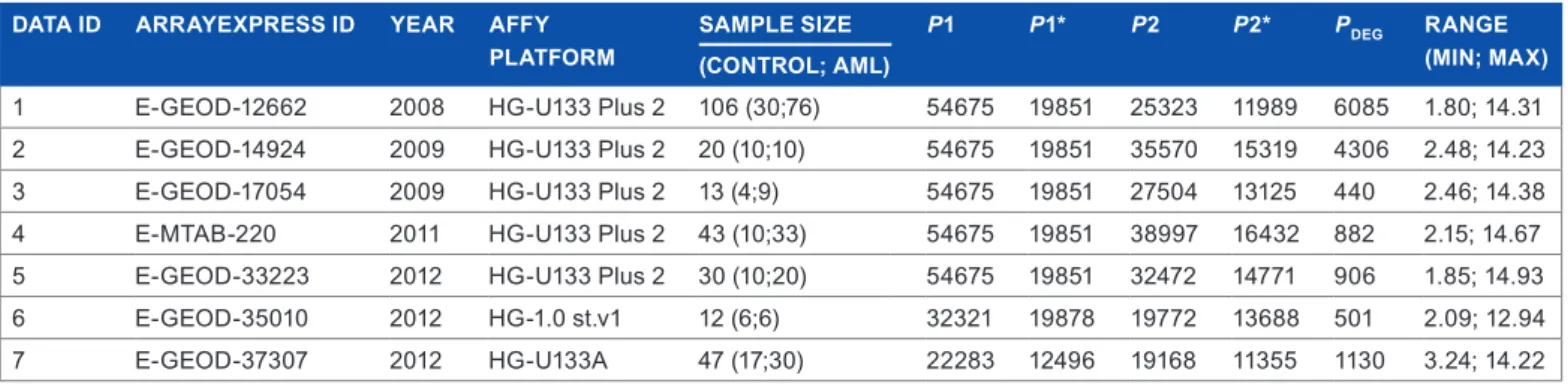
prospective experiment. A new experiment needs to be per-formed when we have not decided yet for all or at least a sub-stantial number of observed genes to be either differentially or nondifferentially expressed, due to insufficient evidence from the experiments done so far to draw a conclusion for each gene. The datasets may be combined from different experi-ments/laboratories and/or collected from systematic search in online repositories. We recommend using raw data to reduce the source of variability due to different preprocessing pro-cedures. We used the downloaded gene expression datasets from ArrayExpress by using acute, myeloid, and leukemia as keywords. We included experiments that had been done in Homo sapiens and had not used DNA by array assay technol-ogy. We left out experiments that had samples without class labels or that had no raw cell files. As a result, we found seven gene expression datasets, as summarized in Table 1 and briefly described below.
E-GEOD-12662. The main objective of this study was to characterize acute promyelocytic leukemia (APL), which is a subtype of AML. The experiment was conducted on 106 sam-ples. The RNA samples were drawn from 76 de novo adult
patients with AML and 30 healthy bone marrow donors.15
E-GEOD-14924. Peripheral blood samples from newly diagnosed patients with AML were used to observe the effect of having AML on the patients’ T cells. The peripheral blood T cells from healthy volunteers served as a control to be com-pared with patients with AML. The study used CD8 and CD4 T cells in the experiment for both patients with AML and normal controls, resulting in four groups with 10 samples each. In our analysis, we took the 20 samples from CD4 T cells from patients with AML and normal controls.16
E-GEOD-17054. Gene expression datasets were obtained from University of Michigan and Stanford University to study dysregulated pathways between normal bone mar-row hematopoietic stem cells (HSC) and leukemic stem cells from patients with AML (AML LCC) samples. A set from Stanford University only was available and therefore included
Step 1 Data collection
Collect the datasets from the possible resources of gene expression studies, eg, using available data from different laboratories and/or doing systematic search from the online repository by following these steps
(i) Define keywords, inclusion and exclusion criteria (ii) Manual screening
(iii) Download gene expression raw datasets
Step 2 Data preparation
(i) Preprocess gene expression raw datasets (ii) Annotate probes
Step 3 Data analysis
(i) Pool gene expression datasets by sequential meta-analysis (ii) Interpret result
figure 1. General proposed approach to apply sequential meta-analysis
to gene expression datasets. the details for each step are described in the methods section.
Table 1. Characteristics of the seven selected microarray experiments.
DATA ID ARRAYExPRESS ID YEAR AffY PLATfoRM
SAMPLE SIzE P1 P1* P2 P2* PDEG RANGE
(MIN; MAx) (CoNTRoL; AML)
1 e-GeoD-12662 2008 HG-U133 Plus 2 106 (30;76) 54675 19851 25323 11989 6085 1.80; 14.31 2 e-GeoD-14924 2009 HG-U133 Plus 2 20 (10;10) 54675 19851 35570 15319 4306 2.48; 14.23 3 e-GeoD-17054 2009 HG-U133 Plus 2 13 (4;9) 54675 19851 27504 13125 440 2.46; 14.38 4 e-mtaB-220 2011 HG-U133 Plus 2 43 (10;33) 54675 19851 38997 16432 882 2.15; 14.67 5 e-GeoD-33223 2012 HG-U133 Plus 2 30 (10;20) 54675 19851 32472 14771 906 1.85; 14.93 6 e-GeoD-35010 2012 HG-1.0 st.v1 12 (6;6) 32321 19878 19772 13688 501 2.09; 12.94 7 e-GeoD-37307 2012 HG-U133A 47 (17;30) 22283 12496 19168 11355 1130 3.24; 14.22
Notes: P1: the initial number of probesets. P1*: the number of unique genes among P1 (replicated genes were summarized by their median). P2: the number
of probesets after filtering. P2*: the number of unique genes among P2 (replicated genes were summarized by their median). PDeG: the number of differentially
expressed genes determined by LImma and fDr 5% for the corresponding gene expression dataset. range: the range of gene expression datasets after normalization and log2 transformation (1).
in our analyses, which contains nine AML LCCs and four normal HSCs.17
E-MTAB-220. C133+ cell fractions were isolated from the bone marrow of 33 patients with AML and 10 healthy donors, and their transcriptional profiles were assessed with Affymetrix HG U133 Plus 2.0. The experiment had been ini-tiated to assess the association of WNT/β-catenin signaling
with AML.18
E-GEOD-33223. Thirty peripheral blood mononuclear cell (PBMC) samples were included in an experiment that was aimed at observing the factors that influence the prognosis in CEBPA-mutated AML. The participants were categorized into three groups, ie, control patients (n = 10), AML patients with multilineage dysplasia (MLD, n = 9), and AML patients
without MLD (n = 11). We regrouped the samples into AML
and normal controls.19
E-GEOD-35010. Short-term (ST-HSC) and long-term HSC (LT-HSC), as well as granulocytic monocytic and pro-genitors (GMP) from patients with AML were compared in gene expression to healthy controls. The gene expression data from the GMP were used in our analysis, with six patients in the AML group and six healthy controls.20
E-GEOD-37307. Microarray gene expression experi-ment was carried out in 30 AML patients and 19 normal HSC donors to identify genes that were differentially expressed between those groups. The gene expression data were obtained either from cryopreserved mononuclear cells or from testis cells. We excluded the two samples that had been obtained from testis cells.
step 2: data preparation. We followed a common
pro-cedure in preprocessing raw gene expression datasets for fur-ther analysis.
Preprocessing data. Methods are widely available for the preprocessing steps, eg, normalization, background correc-tion, and logarithmic transformation. The choices for pre-processing microarray gene expression data have been widely discussed in the literature.21,22 A different choice of prepro-cessing methods may lead to a different result. However, this particular issue will not be covered in this study. The investigator may choose preprocessing methods by familiar-ity, with good knowledge of their properties. In the practi-cal example of our proposed SMA approach, we normalized the raw datasets by quantile normalization, performed back-ground correction according to manufacturer’s platform rec-ommendation, and transformed the expression values to the log2 scale.23 For the Affymetrix platforms, median polish was used as a summarization method of probes into probesets, to deal with outlier probes.24
As is common in microarray studies, we also applied a filtering step to reduce the number of noninformative probe-sets. We only used detection call filtering to minimize the risk of excluding informative genes, ie, we retained all probe-sets whose log2 expression values were greater than 5 in at least 10% of the samples. The differentially expressed genes
resulting from the SMA from filtered and nonfiltered data were then compared.
Gene annotation. Deciding the “objects” to be combined from multiple studies is another point to consider in pooling multiple studies, eg, combining expression values either at the probeset level or at the gene level. Due to the fact that different platforms may have different probeset names for the same genes, we mapped the probesets to the gene level to increase the agreement among the experiments. Since all the selected experiments had been performed on Affymetrix chips, we used the array-specific AffymetrixID by using the Bioconductor package (annotation packages: hgu133plus2.db, hgu133a.db, hugene10stprobeset.db, hugene10sttranscript-cluster.db, and hugene10stv1probe).25 To deal with multiple probesets referring to the same gene, in each experiment we summarized the replicated genes by taking the median of their expres sion values.6
step 3: sequential meta-analysis. In each individual
dataset, we performed a differential expression analysis by fitting a linear model using “limma” in R26 and controlling the false discovery rate at 5%, defined as the expected propor-tion of false rejecpropor-tion among the rejected hypotheses, using the Benjamini and Hochberg (BH) procedure.27 The resulting differentially expressed genes (DEGs) from each study were compared between studies.
Next, we applied an SMA following Whitehead’s bound-aries approach for a double triangular test (TT).28 Sequen-tial design and analysis was originally developed to monitor results of a randomized clinical trial (RCT) in order to draw a conclusion when enough evidence is available. There, the patient is the unit of analysis. The method can also be applied on a higher level, in the setting of a meta-analysis, where the unit of analysis is the study. The method can also be applied to nonrandomized studies. The application of SMA to micro-array experiments is challenging, in the sense that we are deal-ing with thousands of end points (expression value of genes) that are analyzed simultaneously, and far more complex than sequential analysis in the clinical setting, where we usually have a single end point.
As previously described, the SMA is applied to each and every single gene by testing the null hypothesis that the average expression value is equal between two groups against the alternative hypothesis that there is a certain difference in average expression values between two groups. For gene i, the two-sided hypothesis testing is formulated as
H0 :θ =i 0 H1:| |θi =θR
where θi is the standardized mean difference, also known as Cohen’s effect size, between average expression values in the two groups, and θR is the prespecified relevant effect size.29 The same θR is assumed for all the genes. The effect size of gene i in experiment j is estimated as
θij ij ij ij
Y Y
s
= 0− 1, (1)
where Y Yij0
( )
ij1 is the mean of (base 2) logarithmically trans-formed expression values of gene i in Group 0 (1). Whitehead30 defined sij as the square root of the pooled variance estimate of the within-group variances. We, however, adopted the defini-tion of sij as in the limma procedure, by borrowing information of variances from all tested genes. To be more specific, sij is the square root of the shrunken variance to a common variance by applying the empirical Bayes method.31 The estimation of θij is slightly biased in small sample sizes. A common simple correc-tion factor J is J n n ij j j = − +
(
)
− 1 3 4 0 1 9,where nj0 and d nj1 are the sample sizes in Group 0 and Group 1, respectively. The unbiased estimate of the effect size becomes
Jij∗θij, and the variance estimate is redefined as J sij2∗ij2.32 Construction of the double triangular test. The expression values of gene i are analyzed in chronological order of experi-ments. In the TT test, each gene in each experiment contrib-utes to two statistics, namely Z and V, where Z is the efficient score for θi and V is Fisher’s information. The expression val-ues for gene i in experiment j are transformed to Z and V values by the following formulas30:
Z n n Y Y n s V n n n Z n ij j j ij ij j ij ij j j j ij j = 0 1
(
0− 1)
= 0 1− 2 2 * and , (2)where nj is the total sample size in experiment j, ie, nj0+nj1. We defined sij* as the square root of the shrunken variance to a common variance from a limma model with intercept only [while White-head30 defined the s
ij* as the maximum likelihood (ML) standard deviation assuming equal means]. To incorporate heterogeneity, a weight is assigned to Equation (2), which is calculated by
w V ij ij ij = + 1 1 τ 2 .
The newly adjusted Z and V are then defined as Vij* =wij and Zij* =wij ijθ. Methods are available in practice to esti-mate the heterogeneity or between-study variance τij2: eg, the most commonly used method of moments (also known as Der Simonian–Laird (DL) method), restrictive maximum likeli-hood (REML),33 and the variance-component estimator.34 We used the recommended Paule–Mandel (PM) method to estimate the between-study variance.35
The cumulative information from k studies can be entered into a TT test as Zij Z V V j k ij ij j k ij = = = =
∑
∑
1 1 * and *. (3)Cumulative (Zij,Vij) values are then plotted in a TT plot (Fig. 2). The boundaries in a TT are based on three prespeci-fied parameters, namely the type 1 error α, the statistical power (1 −β), and the relevant effect size to be detected θR. We used the computer software PEST36 to calculate the boundaries for the TT with the aforementioned parameters.
A gene i is declared differentially expressed if its sam-ple path [ie, the path of (Z, V)-values] crosses the upper or lower red boundary, and we reject the null hypothesis. We do not reject the null hypothesis if the sample path crosses one of the blue dashed lines (Fig. 2). We are not able to draw a conclusion (yet) if the sample path falls within the boundar-ies. This also implies that more information is needed from future studies.
For a practical example of our proposed approach, we only took fully replicated genes, ie, the genes that appeared in all experiments, in order to visualize the sample path in the TT plot more clearly. As a result, we analyzed 12,211 unduplicated genes sequentially in the nonfiltered datasets. The boundar-ies of the TT were constructed with θrR= 0.8, α= 0.5% and (1 −β ) = 80% (this sequential design is named Design 1). Fur-ther, we applied a Bonferroni correction to α= 5%, resulting in
α= 0.0004%. (with the same levels of θRr and (1 −β ) as men-tioned before) to construct a new sequential design, referred to as Design 2. Additionally, we also applied similar prespecified
40 30 20 10 10 20 30 40 50 60 V Z Do not reject H0 Do not reject H0 Reject H0 Reject H0 0 −10 −20 −30 −40
figure 2. example of a double triangular test (tt) that is designed by
prespecified α,1 −β. and θR. a decision can be made when the sample path crosses one of the boundaries, ie, rejecting the null hypothesis in favor of the alternative hypothesis when it crosses the red lines; and failing to reject the null hypothesis if the sample path crosses the blue dashed lines. no decision can be made if the sample path stays inside the boundaries: then more studies need to be included in the analysis. the
y-axis and x-axis represent the Z and V score, respectively. more detailed explanation for the Z and V score is provided in the methods section.
parameters [θRr = 0.8, (1 − β ) = 80%, for each α = 5% and
α= 5% with Bonferroni correction (equal to α= 0.0007%)] in filtered gene expression data.
results
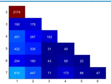
The raw microarray gene expression datasets were collected from the ArrayExpress online repository by using the keywords acute, myeloid, and leukemia, yielding 377 experiments. The number of experiments reduced to 56 after excluding nonhuman experi-ments and had not used DNA by array assay technology (last checked on April 15, 2014). Manual screening of the retained studies resulted in seven microarray experiments that provided raw cell files and had class label in each individual sample. The raw datasets of those experiments were then downloaded. Five datasets were generated from gene expression experiments that had used Affymetrix HG-U133 Plus 2 (54,675 probesets), while the others had used Affymetrix HG-1.0 st. v1 (32,321 probesets) and HG-U133A (22,283 probesets), respectively. Due to different probeset names across platforms, we mapped probesets into the genes level. The number of genes in each dataset after the mapping process is presented in Table 1, as an additional column to the other basic information as well as the number of DEGs in each of seven experiments. We performed pairwise comparisons of the selected differentially expressed genes between the two datasets, and the results are shown in Figure 3. There is a high degree of overlapping informative genes that were obtained by Data 1 and Data 2, ie, 2,174 genes. Meanwhile, there are only 22 genes that were stated as differ-entially expressed genes by both Data 5 and Data 6. Although in general there is a considerable overlap in DEGs between two experiments, we found no gene that was stated as a DEG by all experiments, which confirms our motivation to aggregate the available information as accumulated evidence through SMA.
Based on the cumulative information of the seven experiments that were evaluated by TT using Design 1, with
prespecified parameters θRr= 0.8, α= 0.5%, and (1 −β) = 80%, there are 313 DEGs, 2,838 non-DEGs, and 9,060 genes that needed more experiments in order to draw a conclusion. Of the 12,211 tested genes, the selected α. level yielded an expected number of 62 false-positive genes. Methods for con-trolling the number of false-positive findings are widely avail-able. For α = 5%, with a conservative Bonferroni correction of α= 0.0004% (Design 2), 60 DEGs from the seven experi-ments were found, in which those were also stated as differen-tially expressed genes by Design 1. As compared to Design 1, Design 2 yielded far less DEGs, given the conservative cor-rection in the type 1 error rate for 12,211 tested genes.
The TTs for the two designs in nonfiltered datasets are summarized in Figure 4. The figures are dominated by the orange region, which implies more experiments are to
2174 2 3 4 5 6 7 1 2 3 4 5 6 190 451 422 335 31 49 59 22 47 88 173 71 447 610 43 180 254 287 162 178
figure 3. Pairwise comparisons of the differentially expressed genes
in individual selected experiments. the number within each block represents the overlap of differentially expressed genes between two experiments, which is then represented by the color. the x-axis and
y-axis represent the experiment number.
Cumulative experiments Genes
Cumulative experiments
1 2 3 4 5 6 7 1 2 3 4 5 6 7
figure 4. Heatmaps of the 12,211 fully replicated genes. the colors represent the status of each gene in sequential tests: orange, no decision can be made;
red, do not reject the null hypothesis; white, reject the null hypothesis. the y-axis represents the genes that appeared in all experiments, while the x-axis is the cumulative number of experiments used in the sequential test following Whitehead’s boundaries approach. the boundaries were constructed for a relevant effect size θR= 0.8, power 1 −β= 80%, and a type 1 error α= 0.5% (left) or α= 0.0004% (right, Bonferroni correction for α= 5% and 12,211 tests).
be initiated in order to make a conclusion for the genes of interest, especially when Design 2 is used to construct the tri-angular test.
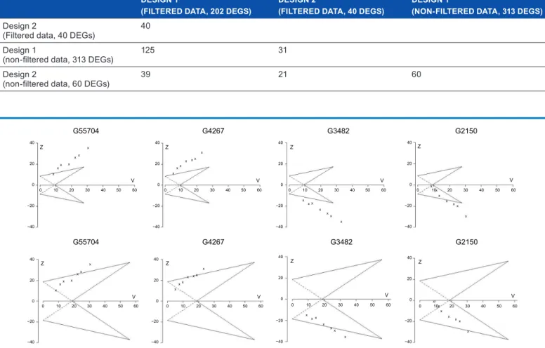
We selected four genes, presented in Figure 5, to show the sample paths of cumulative evidence based on SMA for Designs 1 and 2. The sample paths for the two differ-ent designs are iddiffer-entical in pattern but they do differ in the moment the conclusion can be drawn, due to the fact that the TTs have wider boundaries for the Bonferroni-corrected design. Considering gene G55704 for instance, two experi-ments are enough to decide that the gene is informative when it is evaluated by a TT that was constructed with Design 1. Meanwhile, we need cumulated samples from six experiments in order to draw a conclusion when Design 2 is used to evalu-ate the gene.
We filtered genes with low expression values and took 7,455 genes that appeared in seven experiments. We then performed TTs by applying Design 1. The sequential analy-ses detected 202 genes as DEG, while 1,392 and 5,861 genes were classified as uninformative and undecided, respectively.
When the boundaries of the TT were constructed by
α = 0.0007% (Bonferroni correction for α = 5% in 7,455 tests) with the same relevant effect size and statistical power as in Design 1, we found 40 DEGs with 580 genes classified as uninformative and 6,835 genes that needed more experi-ments in order to make a conclusion. As compared to the nonfiltered data, we found fewer DEGs in the filtered data, which might be due to the exclusion of potential informa-tive genes during the filtering process. The comparisons of the DEGs found based on the nonfiltered and filtered data as well as with and without multiple testing correction are given in Table 2.
discussion
This study has extended the application of SMA into the genomic field. We described and applied the proposed algo-rithm to find potential differentially expressed genes in AML by taking advantage of the public availability of gene expression datasets from published studies as suggested by the MIAME (Minimum Information About a Microarray Experiment)
G55704 40 20 0 0 10 20 30 40 50 60 0 10 20 30 40 50 60 0 10 20 30 40 50 60 0 10 20 30 40 50 60 V V V V Z x Z Z Z x x x x x x x x x x x x x x x x x x x x x x x x x x x −20 −40 40 20 0 −20 −40 40 20 0 −20 −40 40 20 0 −20 −40 0 10 20 30 40 50 60 V Z x x x x x x x 40 20 0 −20 −40 0 10 20 30 40 50 60 V Z x x x x x x x 40 20 0 −20 −40 0 10 20 30 40 50 60 V Z x x x x x x x 40 20 0 −20 −40 0 10 20 30 40 50 60 V Z x x x x x x x 40 20 0 −20 −40 G55704 G4267 G4267 G3482 G3482 G2150 G2150
figure 5. Triangular tests of four selected genes. The boundaries were constructed for a pre-specified effect size θR= 0.8, power 1 −β= 80%, and type 1 error α= 0.5% (the upper row) or α= 0.0004% (the lower row, Bonferroni correction for α= 5%). the y-axis and x-axis represent the Z and V score, respectively. more detailed explanation for the Z and V score is provided in the methods section.
Table 2. Comparisons of the differentially expressed genes that were found with and without incorporating Bonferroni correction in the filtered and non-filtered gene expression data. The numbers represent the number of overlap differentially expressed genes between two different
settings.
DESIGN 1
(fILTERED DATA, 202 DEGS) DESIGN 2 (fILTERED DATA, 40 DEGS) DESIGN 1 (NoN-fILTERED DATA, 313 DEGS)
Design 2
(filtered data, 40 DeGs) 40 Design 1
(non-filtered data, 313 DEGs) 125 31
Design 2
guideline.37 The systematic search in the ArrayExpress online repository and manual screening resulted in seven microarray studies to be analyzed further. We followed a published rec-ommendation6 to conduct a meta-analysis in microarray gene expression data by downloading raw datasets in order to reduce the source of variation due to preprocessing procedures that might vary across experiments.
To the best of our knowledge, application of an SMA (following Whitehead’s boundaries approach) to combine microarray gene expression studies has not yet been employed to detect differentially expressed genes. It is worth mention-ing, however, that sequential analysis has been proposed in single microarray experiments for interim analysis.38 An “ordinary” meta-analysis is also a well-known method to com-bine information from different experiments in genome-wide association studies (GWAS). As mentioned in Introduction, the goal of a meta-analysis is to estimate the effect size (or fold change, in case of differentially expressed gene analysis) without evaluating the adequateness of cumulative evidence to draw a conclusion. The SMA approach could also be a useful tool to decide whether more experiments are needed to draw a conclusion for each and every gene of interest, a property that an “ordinary” meta-analysis lacks.
The effect size described in Equation (1) is similar to the t-statistic to assess the mean difference between two groups, where the denominator is the square root of the pooled variance. The estimation of variance is known to be unstable in small samples. Severe underestimation of vari-ance would inflate the statistic, causing false-positive find-ings. On the other hand, large fold-changed genes would have small statistics if the variance is overestimated. In the analysis of micro array data, empirical Bayes moderated t-statistics came as one of the alternatives to produce stable variances by shrinking extreme variances toward the overall mean variance. Empirical Bayes t-statistics has been proven to outperform ordinary t-statistics.39 Hence, we adopted for the concept of variance estimation from empirical Bayes t-statistics in the estimation of the effect size for each and every gene.
The summaries of the TTs from the 12,211 genes show that almost all the genes need more than one experiment to be declared as either noisy or informative (Fig. 4). Further, the 271 samples from seven experiments are even not enough to draw a conclusion for 9,060 genes when evaluated by Design 1 and 10,994 genes by Design 2 in nonfiltered data. On the other hand, 274 and 55 genes are already classified as redundant genes by single experiments in Designs 1 and 2, respectively. This result also tells us that the signal of expression values differ across the genes. A gene may have a strong signal, so it is easy to be classified as an informative gene without involv-ing a large sample size. Since microarray technology simulta-neously measures thousands of genes, more experiments are needed to cumulatively gather information, particularly for indecisive genes.
Given the curse of dimensionality in microarray studies, filtering redundant genes is commonly applied in practice, eg, removing genes with low variations and/or low expres-sion values.40 The filtering procedure has a risk of exclud-ing the informative genes when gene expression datasets are cumulated across experiments via SMA. This was clearly shown by the identification of some differentially expressed genes on nonfiltered data that were not found in the result of SMA on filtered data. The consequence is even more severe when hard filtering by removing genes with low expression and low variance is applied. Hence, we recommend avoiding any filtering procedure if the computational resources allow doing so.
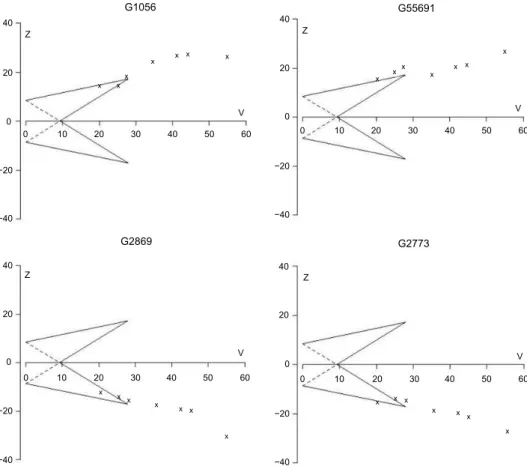
We kept analyzing every gene until information from all experiments was gathered, although the sample paths for some genes had already crossed one of the TT’s boundaries. With the common sequential design, the analysis can be stopped once the sample path crosses a boundary for reason of efficacy or futility. However, investigators might also continue the sequential analysis although the boundary is crossed, in order to optimize the available information, a condition called over-running.28,41 In some genes, the overrunning analysis has as a consequence inconsistency in conclusions. We found genes that were declared noisy genes (non-differentially expressed genes) by TT once they crossed a lower boundary, but then turned out to be informative genes (differentially expressed genes) as more information was accumulated. The inverse case was also found, ie, informative genes became noisy genes when more studies were included. Although more information was gathered and the conclusion changed, the overall fraction of rejected null hypotheses was close to the predetermined type 1 error rate. We provided examples of genes that changed the conclusion when the overrunning analysis was performed (Fig. 6). We also noticed that the phenomenon of a switched conclusion happened only for the genes that had a sample path close to the inner boundary of the TT. We found no gene that crossed both upper and lower boundaries during the sequen-tially cumulated process.
FMS-related tyrosine kinase 3 (FLT3) is an important gene in the development of AML. However, all designs in TTs could not classify FLT3 as being differentially expressed, since the selected cumulative samples could not provide enough information to make a conclusion for this particular gene (Fig. 7). Further, the selected studies15–20 also did not mention this particular gene as a potential biomarker for distinguish-ing patients with AML from normal healthy controls.
The boundaries of a TT depend on prespecified para-meters, namely the effect size, type I error rate, and statisti-cal power. In this study, we used θrR equal to 0.8, which is a relatively large effect size in epidemiological settings.29 It is important to keep in mind that the gene expression data was analyzed on the log2 scale, so that our chosen θRr= 0.8 is equal to a fold change of 1.7 on the original scale. This refer-ence fold change is relatively low compared to the common
G1056 40 20 0 0 10 20 30 40 50 60 0 10 20 30 40 50 60 V V Z Z x x x x x x x x x x x x x x −20 −40 40 20 0 −20 −40 G55691 0 10 20 30 40 50 60 V Z x x x x x x x 40 20 0 −20 −40 G2773 0 10 20 30 40 50 60 V Z x x x x x x x 40 20 0 −20 −40 G2869
figure 6. triangular tests of four selected genes that have inconsistent conclusions. the boundaries were constructed for a relevant effect size θR= 0.8, power 1 −β= 80%, and type 1 error α= 0.5%. the sequential analyses were continued although the sample paths crossed the boundaries (so-called overrunning).28,41
the y-axis and x-axis represent the Z and V score, respectively. more detailed explanation for the Z and V score is provided in the methods section.
0 10 20 30 40 50 60 V Z xxx xxxx 40 20 0 −20 −40 0 10 20 30 40 50 60 V Z x xxx xxx 40 20 0 −20 −40 0 10 20 30 40 50 60 V Z x x xx xx x 40 20 0 −20 −40 0 10 20 30 40 50 60 V Z xx xxxxx 40 20 0 −20 −40
figure 7. Triangular tests for the FLT3 gene. The boundaries were constructed for a prespecified effect size θR= 0.8, power 1 −β= 80%, and type 1 error
α= 0.5% (the first column) or α= 0.0004% (the second column, Bonferroni correction for α= 5%). The first (second) row is the triangular tests when full (filtered) data is used for analysis. The y-axis and x-axis represent the Z and V score, respectively. more detailed explanation for the Z and V score is provided in the methods section.
cut-off value to state a gene as differentially expressed, eg, two or threefold.
Type 1 error is another crucial parameter in the determi-nation of the boundaries of TT. We employed the conserva-tive Bonferroni approach to correct for multiple testing, which depends on the number of tested genes. In the given example, we analyzed the genes that occurred in seven experiments. When a new study is available and Bonferroni correction is applied, the whole process of sequential analysis can be repeated if the investigator would like to include the fully replicated genes only in the analysis. When non-fully-replicated genes (ie, genes that appeared in less than seven experiments) are also included in the analysis, applying Bonferroni correction is most likely to change the conclusions for some previously evaluated genes, since the sequential design is also changed due to different levels of α used. One solution is dividing the chosen classical α= 5%, for instance, by the total number of known genes in the whole genome, which yields an extremely conservative type 1 error rate. The methods involving ordering of the P-values, such as the Benjamini–Hochberg correction, are unfortunately less easy to apply in a triangular test, since we were unable to automatically produce P-values associated with the Z and V statistics in R software. The other option to correct for the multiple testing is to use a lower but less con-servative α, for instance, choosing α= 0.5% rather than the classical α= 5% to reduce false-positive findings.
The TT is one of a group of sequential methods. We specifically chose TT following Whitehead’s boundaries approach. Other similar methods like the sequential probabil-ity ratio test (SPRT) may also be considered. With the same prespecified parameters, it is easier for the SPRT compared to the TT to detect the required effect size earlier in the sequen-tial testing if the effect size is real or if no relevant difference exists. However, TT minimizes the maximum amount of information needed to come to a conclusion compared to the SPRT. We refer to van der Tweel and van Noord42 for further details regarding the comparison of TT and SPRT particu-larly in the case–control study setting. We analyzed the gene expression data also by SPRT and found comparable results with the TT (results are not shown).
We tested gene expression values from different micro-array experiments with a group sequential method. Further, we showed that the time to make a decision varies across the tested genes. This study shows the application of a sequential method in continuous outcome data. Such application may also be extended to count data (Poisson-distributed outcome data, such as in RNA sequencing) or survival outcome data. conclusion
We have shown that samples from one experiment are most likely not enough to classify a gene as informative or nonin-formative. This study showed a method to determine whether there is enough evidence at a certain time point to draw a conclusion for a particular gene or to hold the conclusion
until the evidence is adequate to make conclusion for all the genes under study. SMA following Whitehead’s boundaries approach offers an alternative method to find a gene signature list by evaluating the adequacy of the accumulated evidence. Acknowledgments
The authors would like to thank to S Nikolakopoulos (Bio-statistics and Research Support, Julius Center for Health Sciences and Primary Care, UMC Utrecht) for discussion about group sequential designs. They would also acknowl-edge the anonymous reviewers for their comments and constructive suggestions.
Author contributions
Conceived and designed the experiments: PWN, MJCE, IvdT. Analyzed the data: PWN. Wrote the first draft of the manuscript: PWN. Contributed to the writing of the manu-script: PWN, IvdT, VLJ, KCBR, MJCE. Agreed with the results and conclusions: PWN, IvdT, VLJ, KCBR, MJCE. Jointly developed the structure and arguments for the paper: PWN, MJCE, IvdT. Made critical revisions and approved final version: PWN, IvdT, VLJ, KCBR, MJCE. All authors reviewed and approved of the final manuscript.
references
1. Catherino WH, Segars JH. Microarray analysis in fibroids: which gene list is the correct list? Fertil Steril. 2003;80(2):293–4.
2. Tan PK, Downey TJ, Spitznagel EL Jr, et al. Evaluation of gene expression measurements from commercial microarray platforms. Nucleic Acids Res. 2003; 31(19):5676–84.
3. Fortunel NO, Otu HH, Ng HH, et al. Comment on “‘Stemness’: transcriptional profiling of embryonic and adult stem cells” and “a stem cell molecular signa-ture”. Science. 2003;302(5644):393; author reply 393.
4. Evsikov AV, Solter D. Comment on “‘Stemness’: transcriptional profiling of embryonic and adult stem cells” and “a stem cell molecular signature”. Science. 2003;302(5644):393; author reply 393.
5. Ein-Dor L, Zuk O, Domany E. Thousands of samples are needed to generate a robust gene list for predicting outcome in cancer. Proc Natl Acad Sci U S A. 2006;103(15):5923–8.
6. Ramasamy A, Mondry A, Holmes CC, Altman DG. Key issues in conduct-ing a meta-analysis of gene expression microarray datasets. PLoS Med. 2008; 5(9):e184.
7. Gan Z, Wang J, Salomonis N, et al. MAAMD: a workflow to standardize meta-analyses and comparison of affymetrix microarray data. BMC Bioinformatics. 2014;15:69.
8. Yi SG, Park T. Integrated analysis of the heterogeneous microarray data. BMC Bioinformatics. 2011;12(suppl 5):S3.
9. Li Y, Ghosh D. Assumption weighting for incorporating heterogeneity into meta-analysis of genomic data. Bioinformatics. 2012;28(6):807–14.
10. Chang LC, Lin HM, Sibille E, Tseng GC. Meta-analysis methods for combin-ing multiple expression profiles: comparisons, statistical characterization and an application guideline. BMC Bioinformatics. 2013;14:368.
11. Liu W, Peng Y, Tobin DJ. A new 12-gene diagnostic biomarker signature of melanoma revealed by integrated microarray analysis. PeerJ. 2013;1:e49. 12. Zodro E, Jaroszewski M, Ida A, et al. FUT11 as a potential biomarker of clear
cell renal cell carcinoma progression based on meta-analysis of gene expression data. Tumour Biol. 2014;35(3):2607–17.
13. Borenstein M, Hedges LV, Higgins JPT, Rothstein HR. Cumulative Analysis. Introduction to Meta-Analysis. Chichester, England: John Wiley & Sons, Ltd; 2009:371–6.
14. van der Tweel I, Bollen C. Sequential meta-analysis: an efficient decision-mak-ing tool. Clin Trials. 2010;7(2):136–46.
15. Payton JE, Grieselhuber NR, Chang LW, et al. High throughput digital quan-tification of mRNA abundance in primary human acute myeloid leukemia sam-ples. J Clin Invest. 2009;119(6):1714–26.
16. Le Dieu R, Taussig DC, Ramsay AG, et al. Peripheral blood T cells in acute myeloid leukemia (AML) patients at diagnosis have abnormal phenotype and genotype and form defective immune synapses with AML blasts. Blood. 2009;114(18):3909–16. 17. Majeti R, Becker MW, Tian Q , et al. Dysregulated gene expression networks
in human acute myelogenous leukemia stem cells. Proc Natl Acad Sci U S A. 2009;106(9):3396–401.
18. Beghini A, Corlazzoli F, Del Giacco L, et al. Regeneration-associated WNT signaling is activated in long-term reconstituting AC133bright acute myeloid leukemia cells. Neoplasia. 2012;14(12):1236–48.
19. Bacher U, Schnittger S, Macijewski K, et al. Multilineage dysplasia does not influence prognosis in CEBPA-mutated AML, supporting the WHO proposal to classify these patients as a unique entity. Blood. 2012;119(20):4719–22. 20. Barreyro L, Will B, Bartholdy B, et al. Overexpression of IL-1 receptor
acces-sory protein in stem and progenitor cells and outcome correlation in AML and MDS. Blood. 2012;120(6):1290–8.
21. Bolstad BM, Irizarry RA, Astrand M, Speed TP. A comparison of normaliza-tion methods for high density oligonucleotide array data based on variance and bias. Bioinformatics. 2003;19(2):185–93.
22. Qiu X, Wu H, Hu R. The impact of quantile and rank normalization procedures on the testing power of gene differential expression analysis. BMC Bioinformatics. 2013;14:124.
23. Gautier L, Cope L, Bolstad BM, Irizarry RA. affy – analysis of Affymetrix GeneChip data at the probe level. Bioinformatics. 2004;20(3):307–15. 24. Irizarry RA, Hobbs B, Collin F, et al. Exploration, normalization, and summaries of
high density oligonucleotide array probe level data. Biostatistics. 2003;4(2):249–64. 25. Gentleman RC, Carey VJ, Bates DM, et al. Bioconductor: open software
development for computational biology and bioinformatics. Genome Biol. 2004; 5(10):R80.
26. Bates D, Maechler M. lme4: Linear Mixed-Effects Models Using S4 Classes. R Pack-age Version 0.999375–322009. 2009.
27. Benjamini Y, Hochberg Y. Controlling the false discovery rate: a practical and powerful approach to multiple testing. J R Stat Soc Series B Methodol. 1995;57(1): 289–300.
28. Whitehead J. The Design and Analysis of Sequential Clinical Trials. New York, USA: Wiley; 1997.
29. Cohen J. A power primer. Psychol Bull. 1992;112(1):155–9.
30. Whitehead A. Estimating the Treatment Difference in an Individual Trial. Meta- Analysis of Controlled Clinical Trials. Chichester, England: John Wiley & Sons, Ltd; 2002:23–55.
31. Smyth GK. limma: linear models for microarray data bioinformatics and compu-tational biology solutions using R and bioconductor. In: Gentleman R, Carey V, Huber W, Irizarry R, Dudoit S, eds. Bioinformatics and Computational Biology Solutions Using R and Bioconductor. New York: Springer; 2005:397–420. 32. Borenstein M, Hedges LV, Higgins JPT, Rothstein HR. Effect Sizes Based on
Means. Introduction to Meta-Analysis. Chichester, England: John Wiley & Sons, Ltd; 2009:21–32.
33. DerSimonian R, Kacker R. Random-effects model for meta-analysis of clinical trials: an update. Contemp Clin Trials. 2007;28(2):105–14.
34. Hedges LV. A random effects model for effect sizes. Psychol Bull. 1983;93:388–95. 35. Novianti PW, Roes KC, van der Tweel I. Estimation of between-trial
vari-ance in sequential meta-analyses: a simulation study. Contemp Clin Trials. 2014;37(1):129–38.
36. Whitehead J, Marek P. A FORTRAN program for the design and analysis of sequential clinical trials. Comput Biomed Res. 1985;18(2):176–83.
37. Brazma A, Hingamp P, Quackenbush J, et al. Minimum information about a microarray experiment (MIAME)-toward standards for microarray data. Nat Genet. 2001;29(4):365–71.
38. Marot G, Mayer CD. Sequential analysis for microarray data based on sensitivity and meta-analysis. Stat Appl Genet Mol Biol. 2009;8:Article3.
39. Jeffery IB, Higgins DG, Culhane AC. Comparison and evaluation of methods for generating differentially expressed gene lists from microarray data. BMC Bio-informatics. 2006;7:359.
40. Suarez-Farinas M, Shah KR, Haider AS, Krueger JG, Lowes MA. Personal-ized medicine in psoriasis: developing a genomic classifier to predict histological response to Alefacept. BMC Dermatol. 2010;10:1.
41. Whitehead J. Overrunning and underrunning in sequential clinical trials. Con-trol Clin Trials. 1992;13(2):106–21.
42. van der Tweel I, van Noord PA. Sequential analysis of matched dichotomous data from prospective case-control studies. Stat Med. 2000;19(24):3449–64.