The foundations of lesion-function
inference in the human brain
Institute of Neurology UCL
Submitted in partial fulfilment of the requirement for a degree of Doctor of Philosophy
I, Yee-Haur Mah confirm that the work presented in this thesis is my own. Where information has been derived from other sources, I confirm that this has
Abstract
Understanding the functional architecture of the brain has long been a
challenge in neuroscience with a variety of techniques having been developed to explore this structure-function relationship. However, in order to be able to accurately identify the underlying system we require techniques that have the capabilities of describing the complexities therein.
In order to perform lesion-function studies a cohort of brain scans with the location of the lesion identified must be collected. Utilising diffusion weighted magnetic resonance imaging, normally collected in the clinical setting, I propose a new unsupervised lesion segmentation routine.
The cohort of brain scans also need to be spatially normalised such that homologous regions of the brain are brought into register with each other. However, this process can be perturbed by the presence of a lesion within the scan. Though a series of simulations I evaluate the performance of 12 different spatial normalisation routines on brains scans that possess a lesion.
Historically lesion-function mapping studies have tended to use a univariate statistical approach, where different locations within the brain are treated as being spatially independent from each other. Here I show that biases within the structure of the data have the potential to distort the lesion-function inferences we draw. Though a series of simulations, I show that a mass univariate
technique is vulnerable to these biases and assess three different multivariate methods (Support Vector Machines, Relevance Vector Machines and Flexible Bayesian Modelling) as potential solutions to this problem.
Asides from making lesion-function inferences, these multivariate models can be used to predict future events. Using a data set of paired admission diffusion
weighted magnetic resonance imaging scans and functional outcome scores I apply these techniques to the clinical scenario of predicting the functional outcome of patients after a cerebral vascular event.
Acknowledgements
I am very grateful to Professor Husain and Dr Nachev for supervising this thesis. Their patience and professionalism throughout this process are deeply appreciated.
I am heavily indebted to Dr Nachev, for introducing me to this field of research. Without his generosity and guidance, none of this work would have been possible, and it is to whom I owe my utmost gratitude.
I would also like to extend my thanks to Professor Jackson (Nottingham
University), Dr Yu, So Young Kim and Sun Young Choi (Korea University, Anam Hospital) who kindly assisted in obtaining the data used in §6 of this thesis.
Contents
1 The foundations of lesion-function inference in the human brain 24
1.1 Introduction 24 1.2 Overview 28
1.3 Lesion segmentation 30
1.3.1 Manual segmentation 30
1.3.2 Automated segmentation 31
1.3.2.1 Supervised (semi-automated) segmentation 31 1.3.2.2 Unsupervised (fully automated) segmentation 33
1.3.3 Learning algorithms 34
1.3.3.1 Unsupervised learning algorithms 35
1.3.3.1.1 k-means clustering 35
1.3.3.1.2 Mean-shift clustering 40
1.3.3.2 Supervised learning algorithms 43
1.3.3.2.1 Support Vector Machines 44
1.3.3.2.1.1 The kernel trick 45
1.3.3.2.1.2 Maximum margin / Hyperplane 47
1.3.3.2.1.3 Soft margins 49
1.3.3.2.1.4 Kernel selection 50
1.3.3.2.2 Anomaly measures 52
1.3.3.2.2.1 k-nearest neighbour (k-NN) density estimator 54
1.3.3.2.2.2 Gamma (g) density score 56
1.3.3.2.2.3 Zeta (z) anomaly score 57
1.4 Spatial normalisation 61
1.4.1 Automated spatial normalisation algorithms 61
1.4.1.1 Landmark based methods 62
1.4.1.3 Volume based methods 63
1.4.1.4 Differentiable homeomorphism 64
1.4.2 Spatial normalisation of lesioned brains 64
1.5 Inference 66
1.5.1 Univariate methods 67
1.5.1.1 Template overlay method 68
1.5.1.2 Subtraction overlay method 71
1.5.1.3 Voxel-based Lesion Symptom Mapping (VLSM) 71
1.5.2 Multivariate approaches 74
1.5.2.1 Support Vector Machines 75
1.5.2.2 Relevance Vector Machines 76
1.5.2.3 Comparisons between SVM and RVM 80
1.5.2.4 Bayesian Inference with Markov Chain Monte Carlo sampling 81
1.5.2.4.1 Monte Carlo integration 82
1.5.2.4.2 Markov Chains 84
1.5.2.4.3 Markov Chain Monte Carlo methods 85
1.5.2.4.4 Auto correlation functions and burn in periods 85
1.5.3 Predictive tool 87
1.5.3.1 Cross-validation 87
1.5.4 Assessing model generalizability 89
1.5.4.1 Leave-one-out cross-validation 91
1.5.4.2 k-fold cross-validation 91
1.5.4.3 Split sample cross-validation 92
1.5.4.4 Bootstrapping 93 1.6 Conclusion 95
2 A new method for unsupervised high-dimensional brain lesion
segmentation 97
2.2 Methods 102 2.2.1 Imaging 102
2.2.1.1 Focally lesioned brains 102
2.2.1.2 Non-lesioned reference brains 103
2.2.1.3 Non-lesioned recipient brains 103
2.2.2 Image preprocessing 103
2.2.2.1 Normalisation 103
2.2.2.2 Manual segmentation 106
2.2.2.3 Chimeric image creation 108
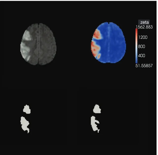
2.2.3 Zeta (z) anomaly score 112
2.2.4 Zeta map thresholding 113
2.2.5 Evaluation 117 2.3 Results 118
2.3.1 Evaluation of the 38 native lesions 118
2.3.2 Evaluation of the 2850 chimeric lesions 120
2.3.2.1 Chimeric images partitioned by lesion 120
2.3.2.2 Chimeric images partitioned by subject 122
2.3.2.3 Visual comparison between the manual segmentation and unsupervised segmentation result for a cortical and
sub-cortical example lesion 124
2.4 Discussion 127 2.4.1 Advantages 127 2.4.2 Disadvantages 129 2.5 Conclusion 132
3 Optimal inter-subject registration of human magnetic resonance brain imaging in the presence of focal lesions 133
3.1 Introduction 133 3.2 Methods 138 3.2.1 Data 139
3.2.1.1 Recipient set 139
3.2.1.2 Donor set 139
3.2.2 Image preprocessing 140
3.2.2.1 Registration of focally lesioned images and binary mask creation 140
3.2.2.2 Chimeric brain creation 141
3.2.2.3 Midline alignment 145
3.2.2.4 Enantiomorphically corrected brain creation 145
3.2.3 Normalisation methods 148
3.2.3.1 Unified segmentation-normalisation 152
3.2.3.2 New segment 153
3.2.4 Evaluation 154 3.3 Results 158
3.3.1 Assessment partitioned according to the background
(recipient) brain scan 158
3.3.2 Assessment partitioned according to the lesion (donor) brain scan 166 3.4 Discussion 192 3.5 Conclusion 197
4 Lesion function mapping using mass univariate techniques 198
4.1 Introduction 198 4.2 Methods 202 4.2.1 Imaging 202
4.2.2 Image preprocessing 202
4.2.3 Data analysis 206
4.2.3.1 Visualisation of a high dimensional data set in two
dimensions 206
4.2.3.2.1 Voxel-wise simulations examining the dependence of a putative function of interest on a single voxel 207
4.2.3.2.1.1 Statistical analysis 210
4.2.3.2.1.2 Calculation of the vector displacement 210 4.2.3.2.1.3 Visualisation of the vector displacement 212 4.2.3.2.2 Brodmann area simulations examining the
dependence of a putative function of interest on a
single cluster of voxels 212
4.2.3.2.2.1 Statistical analysis 212
4.2.3.2.2.2 Calculation of the vector displacement 213 4.3 Results 214 4.3.1 Visualisation of a high dimensional data set in two dimensions
using Isomap and tSNE 214
4.3.2 Mass univariate simulations – Dependence of a putative
function of interest on a single voxel 218
4.3.3 Mass univariate simulations – Dependence of a putative
function of interest on a single Brodmann area 220
4.4 Discussion 223 4.5 Conclusion 226
5 Lesion function inference in the context of spatially
distributed function 227 5.1 Introduction 227 5.2 Methods 232 5.2.1 Imaging 232 5.2.1.1 Image preprocessing 232 5.2.2 Hardware 236 5.2.3 Simulations 236
5.2.3.1 Simulation one : Comparison of mass univariate (Fisher’s exact test) technique against a multivariate
(SVM) technique 237
5.2.3.1.1 Lesion symptom model 237
5.2.3.1.2 Data preparation 237
5.2.3.1.3 Mass univariate analysis (Fisher’s exact test) 237
5.2.3.1.4 Multivariate analysis (SVM) 238
5.2.3.1.5 Comparison of the mass univariate with the
multivariate technique 239
5.2.3.2 Simulation two : Comparison of different multivariate
techniques 240
5.2.3.2.1 Lesion symptom model 240
5.2.3.2.2 Data preparation 240
5.2.3.2.3 Support Vector Machines (SVM) 241
5.2.3.2.4 Relevance Vector Machines (RVM) 242
5.2.3.2.5 Flexible Bayesian Modelling (FBM) 242
5.2.3.2.6 Comparison of SVM, RVM and FBM 243
5.3 Results 245 5.3.1 Simulation one : Comparison of a mass univariate
(Fisher’s exact test) technique against a multivariate
(SVM) technique 245
5.3.1.1 Mass univariate analysis (Fisher’s exact test) 245
5.3.1.2 Multivariate analysis (SVM) 254
5.3.2 Simulation two : Comparison of different multivariate
techniques 256
5.3.2.1 Support Vector Machines (SVM) 257
5.3.2.2 Relevance Vector Machines (RVM) 265
5.3.2.3 Flexible Bayesian Modelling (FBM) 269
5.3.2.4 Predictions 279 5.4 Discussion 280
5.4.1 Simulation one : Comparison of a mass univariate technique (Fisher’s exact test) with a multivariate technique (SVM) 281 5.4.2 Simulation two : Comparison of three different multivariate
techniques on a two loci model 281
5.5 Conclusion 284
6 Post stroke outcome prediction using acute stroke imaging and high-dimensional multivariate algorithms 285
6.1 Introduction 285 6.2 Methods 289 6.2.1 Hardware 289 6.2.2 Data 289
6.2.2.1 National Hospital for Neurology and
Neurosurgery images 289
6.2.2.2 Korea University Anam Hospital images 290
6.2.2.3 Outcome data : Barthel Index 292
6.2.3 Image preprocessing 292
6.2.4 Support Vector Machine model generation 293
6.2.4.1 Classification of patients’ outcome into dependent and
independent groups 293
6.2.4.2 Support Vector Machine based on a linear kernel 293 6.2.5 Evaluation 296
6.2.5.1 Visualisation of the weights associated with
each dimension 298
6.3 Results 299 6.3.1 Functional independence described as a Barthel index of
6.3.2 Functional independence described as a Barthel index of
greater than or equal to 60 302
6.3.3 Functional independence described as a Barthel index of
greater than 40 305
6.3.4 Visualisation of the weights extracted from the Support Vector
Machine model 308
6.4 Discussion 312 6.5 Conclusion 315
7 Conclusion 316
7.1 Spatial biases within lesion imaging data 317
7.2 Automation of image analysis 320
7.3 Inference and prediction 322
7.4 Future work 324
8 Appendix 326
8.1 Appendix A 326
8.2 Appendix B 329
8.2.1 Statistical Parametric Mapping 5 (SPM5) settings 329
8.2.1.1 SPM5 co-registration defaults 329
8.2.1.2 SPM5 preproc (unified segmentation-normalisation routine) 329 8.2.2 Statistical Parametric Mapping 8 (SPM8) settings 330
8.2.2.1 SPM8 Segment 330 8.2.2.2 SPM8 Co-register 330 8.2.2.3 SPM8 Normalise 331 8.2.2.4 SPM8 Reorient 332 8.2.3 SPM8 settings used in §2 335 8.2.3.1 Unified Segment
8.2.3.2 Create deformation field from sn file
[ULP, ULPD, ULC, ULCD, ULE, ULED] 336
8.2.3.3 Import tissue classes for use with DARTEL
[ULPD, ULCP, ULED] 336
8.2.3.4 Create DARTEL Templates
[ULPD, ULCD, ULED] 338
8.2.3.5 Transform the DARTEL flow field into MNI space 339 8.2.3.6 Create deformation field from DARTEL flow field
[ULPD, ULCD, ULED] 340
8.2.3.7 New Segment
[NSPD, NWPD, NSED, NWED] 341
List of Figures
1 The foundations of lesion-function inference in the human brain
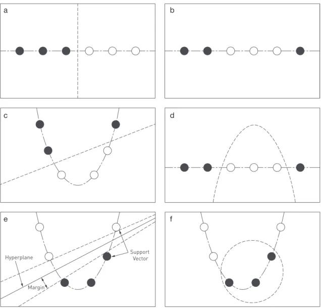
Figure 1.1 k means clustering 36
Figure 1.2 Mean shift clustering 41
Figure 1.3 Support Vector Machines (SVM) 46
Figure 1.4 k-nearest neighbour (k-NN) 55
Figure 1.5 Gamma (g) and Zeta (z) anomaly score 58
Figure 1.6 Template overlay method 70
Figure 1.7 Illustraion of under-fitting and over-fitting 90
2 A new method for unsupervised high-dimensional brain lesion segmentation
Figure 2.1 Lesion coverage map 107
Figure 2.2 Chimeric image creation flow diagram 110
Figure 2.3 Table of abbreviations for figure 2.2 111
Figure 2.4 Outline of zeta segmentation method 116
Figure 2.5 Native brain performance 119
Figure 2.6 Chimeric brain performance partitioned by lesion 121
Figure 2.7 Chimeric brain performance partitioned by subject 123
Figure 2.8 Zeta segmentation (cortical) 125
3 Optimal inter-subject registration of human magnetic resonance brain imaging in the presence of focal lesions
Figure 3.1 Image preprocessing 142
Figure 3.2 Table of abbreviations for figure 3.1 144
Figure 3.3 Enantiomorphically corrected image creation 147
Figure 3.4 Table of abbreviations for the different
normalisation methods 149
Figure 3.5 Unified segmentation-normalisation routine base
methods 150
Figure 3.6 New segment routine base methods 151
Figure 3.7 Unified segmentation-normalisation routines
(recipient): mean root mean squared differences 160
Figure 3.8 Unified segmentation-normalisation and DARTEL routines (recipient): mean root mean squared
differences 161
Figure 3.9 New segment and DARTEL routines (recipient):
mean root mean squared differences 162
Figure 3.10 Unified segmenation-normalisation routines
(recipient): mean volume change ratios 163
Figure 3.11 Unified segmentation-normalisation and DARTEL routines (recipient): mean volume change ratios 164
Figure 3.12 New segment and DARTEL routines (recipient):
Figure 3.13 Unified segmentation-normalisation routines:
Log10(RMSD) vs Log10(lesion volume) 168
Figure 3.14 Unified segmentation-normalisation and DARTEL routines: Log10(RMSD) vs Log10(lesion volume) 169
Figure 3.15 New segment and DARTEL routines:
Log10(RMSD) vs Log10(lesion volume) 170
Figure 3.16 ANCOVA comparing ULPD and ULED 172
Figure 3.17 ANCOVA comparing NSPD and NSED 173
Figure 3.18 ANCOVA comparing ULPD and ULCD 175
Figure 3.19 ANCOVA comparing ULP and ULE 177
Figure 3.20 ANCOVA comparing ULP and ULC 178
Figure 3.21 ANCOVA comparing ULE, ULED and NSED 180
Figure 3.22 ANCOVA comparing ULC and ULCD 181
Figure 3.23 ANCOVA comparing ULC and ULE 183
Figure 3.24 ANCOVA comparing ULC, ULE, NSED and ULCD 184
Figure 3.25 Unified segmentation-normalisation routines:
mean volume change ratio vs Log10(lesion volume) 186
Figure 3.26 Unified segmentation-normalisation and DARTEL routines:
mean volume change ratio vs Log10(lesion volume) 187
Figure 3.27 New segment and DARTEL routines:
Figure 3.28 2 sample t-test assessing ULC vs ULE and
ULC vs ULED 190
Figure 3.29 2 sample t-test assessing ULC vs ULE 191
4 Lesion function mapping using mass univariate techniques
Figure 4.1 Lesion overlay map of the 581 lesion masks 204
Figure 4.2 Lesion overlay map of the 581 lesion masks
collapsed on the right hemisphere 205
Figure 4.3 Flow diagram illustrating the single voxel dependence of a putative function of interest
simulation 209
Figure 4.4 Illustration for the calculation of the centre of
mass 211
Figure 4.5 A 2 dimensional embedding of the high
dimensional data set of 581 brains using tSNE
(lesion volume) 216
Figure 4.6 A 2 dimensional embedding of the high
dimensional data set of 581 brains using tSNE
(lesion location) 217
Figure 4.7 Displacement vector map for the simulation using a single voxel dependence of a putative function
of interest 219
Figure 4.8 Table of the displacement means, standard deviations and inter-quartile ranges for the 41
Figure 4.9 Plot of the mean displacement for 41 Brodmann areas as a function of minimum percentage
volume involvement 222
5 Lesion function inference in the context of spatially distributed function
Figure 5.1 Lesion overlay map of the 581 lesion masks 234
Figure 5.2 Lesion overlay map of the 581 lesion masks
collapsed on the right hemisphere 235
Figure 5.3 Plots comparing univariate (left) and
multivariate (right) models: peak 247
Figure 5.4 Plots comparing univariate (left) and
multivariate (right) models: 5% 248
Figure 5.5 Plots comparing univariate (left) and
multivariate (right) models: 10% 249
Figure 5.6 Plots comparing univariate (left) and
multivariate (right) models: 20% 250
Figure 5.7 Plots comparing univariate (left) and
multivariate (right) models: 40% 251
Figure 5.8 Plots comparing univariate (left) and
multivariate (right) models, with the superior
temporal gyus outline: 20% 252
Figure 5.9 Plots comparing univariate (left) and
multivariate (right) models, with the superior
Figure 5.10 Receiver operating curve comparing the
univariate and multivariate models 255
Figure 5.11 Plots comparing SVM and FBM models:
peak and 5% 258
Figure 5.12 Plots comparing SVM and FBM models:
10% and 15% 259
Figure 5.13 Plots comparing SVM and FBM models:
20% and 30% 260
Figure 5.14 Plots comparing SVM and FBM models:
40% and 50% 261
Figure 5.15 Plots comparing SVM and FBM models:
peak, 5%, 10%, 15% 264
Figure 5.16 Plots comparing SVM and FBM models:
20%, 30%, 40%, 50% 264
Figure 5.17 Plot displaying the RVM model: sagittal plane 267
Figure 5.18 Plot displaying the RVM model: axial plane 268
Figure 5.19 Autocorrelation functions for 12 randomly selected voxels from the FBM 1000 iteration model 270
Figure 5.20 Autocorrelation functions for 12 randomly selected voxels from the FBM 2000 iteration model 271
Figure 5.21 Mean trace plot for the FBM 1000 iteration model 273
Figure 5.22 Mean trace plot for the FBM 2000 iteration model 274
Figure 5.24 Autocorrelation function for the FBM 2000 model 276
Figure 5.25 Receiver operating curve comparing the
SVM, FBM1000 and FBM2000 models 278
Figure 5.26 Table showing the predictive performance of the
4 different multivariate models 279
6 Post stroke outcome prediction using acute stroke imaging and high-dimensional multivariate algorithms
Figure 6.1 Lesion coverage map 291
Figure 6.2 Cross-validation flow diagram 295
Figure 6.3 Plots showing sensitivity, specificity and accuracy as a function of the C parameter for an SVM model based on a linear kernel: independence
specified as a BI equal to 100 300
Figure 6.4 Plots showing positive predictive value, negative predictive value and accuracy as a function of the C parameter for an SVM model based on a linear kernel: independence
specified as a BI equal to 100 301
Figure 6.5 Plots showing sensitivity, specificity and accuracy as a function of the C parameter for an SVM model based on a linear kernel: independence
Figure 6.6 Plots showing positive predictive value, negative predictive value and accuracy as a function of the C parameter for an SVM
model based on a linear kernel: independence
specified as a BI greater than or equal to 60 304
Figure 6.7 Plots showing sensitivity, specificity and accuracy as a function of the C parameter for an SVM model based on a linear kernel: independence
specified as a BI greater than 40 306
Figure 6.8 Plots showing positive predictive value, negative predictive value and accuracy as a function of the C parameter for an SVM
model based on a linear kernel: independence
specified as a BI greater 40 307
Figure 6.9 Colour map of SVM model: Functional independence described as a Barthel Index
equal to 100 309
Figure 6.10 Colour map of SVM model: Functional independence described as a Barthel Index
greater than or equal to 60 310
Figure 6.11 Colour map of SVM model: Functional independence described as a Barthel Index
7 Conclusion 8 Appendix
Figure 8.1 Descriptive statistics of stroke lesion
segmentation results on diffusion weighted
MR images 327
Figure 8.2 Table of mislocalisation for each Brodmann area calculated from the dataset of 581 lesion masks 328
1
The foundations of
lesion-function inference in the
human brain
1.1
Introduction
Lesion-function inference refers to understanding the localisation of function in the human brain with the aid of lesions. Over the history of neuroscience a variety of techniques has contributed to our current understanding of this functional architecture. The first of these, historically, were lesion studies that examined the relationship between regions of localised injury and the observed behaviour or functional deficits exhibited by the afflicted patients. In the past, lesion studies relied on post mortem examination of the patient’s brain to
identify the anatomy of the lesion (Broca, 1861; Wernicke, 1874). However, with the development of non-invasive brain imaging such as computer tomography (CT) and magnetic resonance imaging (MRI), the regions of damage could be examined in vivo, therefore not only improving the spatial resolution of the technique but also facilitating the collection of suitable control subjects (Bates et al., 2003; Bird et al., 2006; Rorden and Karnath, 2004). In parallel with this, other techniques for functional brain mapping such as transcranial magnetic stimulation (TMS), transcranial direct current stimulation (tDCS) and especially functional magnetic resonance imaging (fMRI) have emerged: as a result it would be an understatement to say that lesion studies have faded in popularity, particularly relative to fMRI. The question I wish to examine here is whether or
not, and to what extent, lesion mapping remains a valuable tool for determining the functional architecture of the brain.
Functional magnetic resonance imaging (fMRI) has become a popular tool for investigating the functional architecture of the brain as it provides a non-invasive approach to visualising, in vivo, the functioning brain (Heeger and Ress, 2002; Matthews and Jezzard, 2004). The technique relies on the different magnetic properties of oxygenated and deoxygenated haemoglobin – blood oxygen level dependent (BOLD) signal – and the association between increased neuronal activity and local changes in oxygen saturation. Critically, the BOLD signal is only an indirect measure of neuronal activity and may be influenced by many factors not captured in the experimental design. In addition, the signal measured appears to be related principally to input, rather than output, from the neural tissue (Logothetis, 2003), reflecting only a limited aspect of neural function. In comparison with lesion studies where the experimenter is confident that the injured areas are no longer functional, the degree of certainty with fMRI with regards to the level of involvement of an identified region is far more variable. Most importantly, even where BOLD is a reliable indicator of neural function the presence or absence of activity can only be correlated with a function of interest. A correlation establishes neither necessity nor sufficiency for any function: the two conditions that need to be satisfied for any substrate to be argued to mediate a given function. As a result, fMRI is useful in identifying candidate regions potentially critical for a function, i.e. generating hypothetical functional models of the brain, but less useful in discriminating between them. Logically, in order to test whether a specific region is critical for a particular function, one must be able to show the loss of function (or expression of the symptom) when the region is inactivated (Aue et
al., 2009). For strong inference we must therefore turn to techniques that either generate or exploit disruption of brain function.
Transcranial magnetic stimulation (TMS) is a non invasive procedure that renders a region of the brain dysfunctional by the application of a rapidly changing magnetic field over the exterior surface of the skull (Walsh and Cowey, 2000). The fluctuating magnetic field causes the depolarization and hyperpolarizaton of the neurons directly beneath the electric coil, temporarily disturbing the normal functioning of the region of brain. The ability to examine the same brain in the two different states significantly increases the inferential power of the technique as it allows within-subject comparisons, although it should be appreciated that the reported behavioural effects of TMS have largely been on increasing reaction time, rather than altering other aspects of performance (e.g. errors). However, the anatomical range of TMS is limited, particularly in depth, as the effects of stimulation are confined to superficial cortical regions and cannot be used to investigate deep medial or subcortical structures (Epstein et al., 1990; Rudiak and Marg, 1994; Walsh and Cowey, 2000; Zangen et al., 2005). Furthermore, if we were to treat the surface of the brain as a two dimensional surface, the effect of TMS within this plane would always be ill-defined, as the extent of influence exerted by a magnetic field decreases logarithmically with increasing distance from the source (Sack and Linden, 2003).
Procedural modifications have been developed to counteract this issue, include stimulating multiple overlapping regions and determining the localization of the behaviour by subtractive inference, thereby improving the spatial resolution to the order of millimetres. However, it should be borne in mind, that the surface of the brain consists of multiple folds and overlapping gyri, greatly complicating the modelling of field spread. Furthermore, although a specific region of the cortex is stimulated by the TMS coil, the relation of this region to the functional
outcome may not be direct. Remote cortical and subcortical regions may be implicated in generating the observed outcome in a complex network via a series of connections, impacting on the spatial specificity of the technique (Paus et al., 1997; Ruff et al., 2009). Although multiple stimulation sites may be used to help improve the spatial resolution, there is still a practical limitation to the total number of sites one can stimulate concurrently. This will also place a restriction on our ability to test multiple site localisation.
Similar difficulties complicate transcranial direct current stimulation (tDCS), which involves applying an electric current between two electrodes over the surface of the skull to modulate the brain tissue between them (Utz et al., 2010). Unlike TMS, it does not induce polarization and hyperpolarization of the underlying neurons, but modulates their resting potential, thereby modifying the excitability of the neurons. A further difficulty here is the uncertainty about the location of these effects: any region of the brain between the electrodes may be affected. As a tool for making anatomical inferences about brain function its power is necessarily limited.
These objections are not exhaustive. But they give us enough grounds to return to lesion-function mapping as a technique that can provide both
anatomical precision and strong inferential power to test the many hypotheses generated by functional imaging. Though lesions in the human cannot be induced experimentally (for obvious ethical reasons) there is a wealth of such data in clinical populations, in particular from cerebrovascular injury. We need to consider how such data should best be used to make lesion-function inferences in the human brain.
1.2
Overview
In order to make inferences that may be generalised to the population, studies involving cohorts of multiple patients are required (Rorden and Karnath, 2004). As a consequence, unlike single case reports, the neuro-imaging data must be appropriately preprocessed into a format suitable for analysis across a group. The journey from data to inference can be divided conceptually into 3 broad steps. First, the lesioned regions of the brain must be differentiated from the healthy parts. This process of identifying lesioned from healthy tissue is known as lesion segmentation (Fiez et al., 2000). Second, the anatomical labels of the brain must be identified. This is achieved by bringing the imaging data into register with a standard labelled template through a process also known as spatial normalisation (Ashburner and Friston, 1997, 1999; Friston et al., 1995). This ensures homologous parts of the brain are aligned and in register with a known map, so as to allow across-subject comparisons. Third are the statistical calculations that are performed on the preprocessed data: the lesion-function inference proper (Rorden and Karnath, 2004).
Though these are, conceptually speaking, simple practicalities it should be borne in mind that the context is complex. Any study here is dependent on the anatomical consistencies – across subjects – of the functional specialization within the brain. If no relationship – consistent amongst
different people – exists, no technique comparing groups will be able to find one. The preprocessing steps aim to minimize the noise introduced into the process and thus to improve our ability to identify true relationships: but that is as far as they go. Furthermore, the structure-function relationships our inferential techniques use to model the brain must be sensitive to the potential relationships that may exist. In the syndrome of visusospatial neglect (in which patients fail to pay attention towards contralesional space), for example, the effects of a symptomatic lesion in the right parietal lobe can be reversed by
a second lesion in the left frontal lobe (Vuilleumier et al., 1996). This would suggest that the brain is not limited to simple monotonic relationships, but has the potential for far more complex, non-monotonic interactions within distributed systems. Our inferential techniques used to model the brain must be able to handle these possibilities. Critically, any bias introduced into the system, such as through the sampling of the lesions, is of grave concern as these effects unlike noise will persist or even amplify as the data set is increased.
1.3
Lesion segmentation
Lesion segmentation is the process of differentiating between healthy and injured tissue, and is essential before any spatial inference about the behavioural effects of a lesion can be made. Inevitably, in clinical practice it reduces to the question of normal vs abnormal brain image signal, for we do not ordinarily have any other means of exploring the human brain in vivo (Bhanu Prakash et al., 2008; Fiez et al., 2000). The difficulty is that it is not just the signal abnormality at a given point, but the pattern across the brain, that would naturally compel us to label an area as damaged. For example, an island of normal tissue within a damaged area might have entirely normal signal but clearly cannot be functional, for it will be disconnected from the rest of the brain. This kind of complexity, (quite apart from the difficulty of analysing brain images even in terms of isolated signal abnormalities), means the gold standard is manual segmentation: doing it by eye (Mort et al., 2003). With this in mind, it is clear that the process of segmentation and registration are closely intertwined, since deciding whether an area is injured or abnormal relies on comparing its appearance with what we would normally expect to find at that location. There is also the issue of the definition of an abnormal signal itself being contextual, and not an absolute value. Not only do brains differ from one person to the next in the normal population, but from a technological stand point it is particularly relevant with magnetic resonance imaging, as there is no standard signal scale.
1.3.1
Manual segmentation
Manual segmentation refers to the process of lesion segmentation performed by a person. A trained operator draws around a lesion on the basis of
his expertise, whatever it is that might be said to consist in. The obvious difficulty of not having a perspicuous set of criteria aside, this approach is
labour intensive, rendering large scale analyses infeasible. Moreover, the flexibility that gives manual segmentation its strength is also the source of its greatest weakness: the structure of any bias in drawing around the lesion is unpredictable (itself being very complex), and the variability shows the potential for bias is not insubstantial (Van Leemput et al., 2001; Tan et al., 2002). Indeed, one study examining intra and inter- operator variability on a small set of 10 brains, defined as the percentage of non-overlapping voxels between the binary masks derived from the same lesioned brain image, found a mean variability of 31% and 33% respectively. This is certainly potentially large enough — if associated with bias — to distort data (Fiez et al., 2000).
1.3.2
Automated segmentation
The case in favour of avoiding manual segmentation can be made with ease; the question is what should take its place. We now look at various approaches, in order of decreasing requirement for human input (supervision).
1.3.2.1 Supervised (semi-automated) segmentation
Supervised (semi-automated) segmentation is a very broad category, with a range of computer assistance offered to the operator. Methods to simplify the more complex task of delineating the normal-abnormal boundary have been attempted with algorithms that work “on-the-fly”, guided by the operator’s hand (Barrett and Mortensen, 1997; Falcao et al., 1998, 2000). Whilst the operator assesses the image and identifies “seeds” along the boundary line, the algorithm uses these “seeds” to calculate its own boundary line based on local information, adjusting in real-time the position of the boundary line placement. The operator can then, if necessary, review and adjust sections of the boundary at will. One such method, the ultra fast user-steered “live wire on-the-fly”, allows the operator to visualize the position of the boundary line
calculated as he moved the cursor around the 2d image (Falcao et al., 2000). This arrangement resulted in an increase in operator accuracy, a reduction in variability and a significant drop in time costs of the magnitude of 1.2—31 times.
Alternative supervised methodologies have looked at further reducing operator involvement by trying to completely automate boundary extraction. One such example is by Filippi et al. (Filippi et al., 1995). Here they looked at the effect of (a relatively simplistic method of) computer assisted segmentation on intra- and inter-operator variability. Assistance took the form of a rudimentary thresholding method which subsequently required manual post processing to refine the lesion edge. Just as Fiez et al found, there was indeed intra- and inter-operator variation, but more importantly they reported that their computer assisted method reduced both these forms of variation. Unlike the earlier described method, the first-pass boundary extraction has been performed largely by the algorithm alone, with refinements performed on a second pass analysis.
More recently Ashton et al. (Ashton et al., 2003) examined the performance of 2 semi-automated techniques against manual segmentation, looking specifically at the inherent variability of each method. The first of these semi-automated methods, geometrically constrained region growth (GEORG), required the operator simply to identify each of the lesions present in the brain volume with a single mouse click. The algorithm would subsequently identify the boundaries of each of the lesions flagged by the operator. In the second, directed multispectral segmentation (DMSS), an example lesion within the brain volume needed to be first delineated by the operator (either manually or semi-automated), with the algorithm then searching the rest of the brain volume for further lesions. This method proved itself to be very useful to screen for any missed lesions, particularly in diseases like multiple sclerosis, where
there are usually multiple lesions, but was less helpful in diseases generally characterized by a single lesion. Nevertheless, manual segmentation was shown to exhibit the most amount of intra- and inter-operator variability, with both semi-automated algorithms displaying improved accuracy and reduced variability on artificially lesioned brain volumes. The authors suggested that some of the variability was due to the remaining operator involvement as the DMSS algorithm is dependent on the lesion selected and the GEORG method required the operator identifying each lesion within the brain.
It may be paradoxical that these studies focus on measures of operator
variability while retaining the one element sure to guarantee it: the involvement of any kind of operator. Despite the improvements seen, a completely
automated procedure is clearly the only answer to the problem of unknown bias from an operator. It is to these algorithms that I will dedicate greater space, looking at the various methodologies currently available to us and later examining how they have been adapted to the problem of lesion segmentation.
1.3.2.2 Unsupervised (fully automated) segmentation
The process of labelling an image without the aid of an operator — whether in terms of diseased vs normal or not — is termed unsupervised segmentation. Since there is nothing or little but the data to guide the labelling process, its theoretical background falls within the domains of supervised and
unsupervised learning algorithms. With advancements in digital imaging and computing power following Moore’s law (where the number of transistors on an integrated circuit doubles approximately every 2 years), there has been increasing interest in developing computer algorithms to fully automate the process. Irrespective of current hardware / technological limitations, designing a fully automated algorithm is still not an easy task. The problems with these algorithms reduce to 3 main points: first, there is no clear definition of what
is correct and what is not. Unless a “ground-truth” answer is available, it is difficult to differentiate between the appropriateness of one result compared with another, particularly with high dimensional data. The feature(s) one algorithm prioritises over another is often unknown to the operator and deciding which of these (abstract) measures is more pertinent is open to debate. All that is amenable to comparison is the final result. Second, these algorithms are very sensitive to the dimensionality of the data set. As the number of dimensions increase, the algorithm must search a more complex feature space, thereby increasing the computational load, generally in a non-linear fashion, and reducing the probability a good solution may be found. Lastly, these algorithms are sensitive to the parameters of the process. A fully automated method is akin to a ballistic motor action. The operator must first set the parameters of the algorithm prior to its execution, and then await the final output result. Although not all these parameters are problematic to identify, some pose significant obstacles to complete automation. For example returning to the semi-automated technique of GEORG the algorithm needs to know a priori the number of lesions present in the data set (Ashton et al., 2003).
There is an entire mathematical field dedicated to learning algorithms and I do not claim to provide a comprehensive review (Duda and Hart, 1973; Forgy, 1965; MacKay, 2003; MacQueen, 1967). The following sections aim to provide an introduction to some of the concepts behind the mathematics and how their restrictions may impinge on their applicability to the task of lesion segmentation.
1.3.3
Learning algorithms
To differentiate between healthy and damaged tissue, segmentation algorithms must learn some feature(s) that separates them. Although a complete profile of differences would be optimal, it is not necessary and often not possible
with the data available. Careful consideration is required to appropriately parameterise the data to facilitate the identification of these discriminatory features. Broadly speaking, learning algorithms can be divided into two groups – unsupervised and supervised algorithms – depending on the source of the information on which the discrimination is made.
1.3.3.1 Unsupervised learning algorithms
Unsupervised techniques are methods that do not require a priori knowledge of the sub groups within the data, using only the information contained within the test data itself. They are also referred as clustering algorithms, identifying structure within the data without the aid of a separate label. Though many such algorithms have been proposed, here I examine two that have found application within our field of interest: k-means clustering (Forgy, 1965; MacQueen, 1967) and mean-shift clustering (Fukunage and Narendra, 1975).
1.3.3.1.1 k-means clustering
K-means clustering is an iterative algorithm that seeks to partition a dataset into a fixed number (k) of groups and achieves this by minimizing some measure of within-group dissimilarity (Forgy, 1965; MacQueen, 1967). By knowing the number of centres within the data set, the algorithm seeks to minimize the maximum distance of every point from its closest centre. Data points are then grouped into their most appropriate cluster where the objective is to minimize the sum distance from its centre.
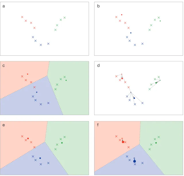
Figure 1.1 - k-means clustering.
The following 6 panels illustrate the process of k-means clustering. The above example displays a collection of 12 data points distributed in a 2 dimensional feature space, with a single feature along the horizontal and vertical axis. There are 3 groups within the dataset represented by a different colour. The starting locations of the centroids can either be explicitly specified or randomly determined. Since k=3, there are three centroids, represented as a filled circle, in this scenario (b). The algorithm then proceeds to assign each data point to the closest of the three centroids using a series of perpendicular bisectors (c). After all data points have been assigned, the centroids’ locations are then shifted to the mean location of the corresponding centroid groups (d and e), and the process is repeated until no further displacement occurs (f).
a c e b d f
37
Consider a dataset distributed in 2-dimensional space with one feature along the x axis and another along the y as illustrated in figure XX. The value of k refers to the number of starting points (centroids) the algorithm will use to explore the feature space. This is essence
specifies the maximum number of clusters you expect to find within the dataset. The example in figure XX uses a k value of 3. Next the data points are then assigned to their closest centroid by using a series of perpendicular bisectors resulting in the formation of 3 clusters based on the entire dataset. For each cluster the associated centroid is updated to the mean of its constituent data points. The process is then repeated, slowly moving each centroid to the minimum distortion point (MacKay 2003) with termination of the process defined by a minimum displacement. In this way the algorithm does not necessarily need to evaluate all ������
� pair-wise dissimilarities.
To evaluate the displacement between iterations, a method to calculate the distance is necessary ���� �� �12 ����� ���� � Variables used: ����� ���� ����� ���� � ��� �� ��������� ��� ������ ����� ������� �������� ��� ������� ������� ������ �������� ��� �������� ���� ����� �� �������� �� ������ �� ������ ��������� �������� ����������� ����� �������� � ��������� �� ���������
Each data point is assigned to the nearest centroid within the set of centroids using the distance measure above.
������ ������
� �������� ������ ������ �1 �� ������ �
� �� ������ �
After assigning each data point to its closest centroid, the means are adjusted to match the sample means of the data points they are responsible for, i.e. the locations of the set of centroids are updated.
�����∑ �� �������� ���� Here ���� is the total responsibility of the mean k.
Consider a dataset distributed in 2-dimensional space with one feature along the x axis and another along the y as illustrated in figure 1.1. The value of k refers to the number of starting points (centroids) the algorithm will use to explore the feature space. This in essence specifies the maximum number of clusters you expect to find within the dataset. The example in figure 1.1 uses a k value of 3. The starting locations of the centroids can either be specified by the operator or randomly determined. Next the data points are then assigned to their closest centroid by using a series of perpendicular bisectors resulting in the formation of 3 clusters based on the entire dataset. For each cluster the associated centroid is updated to the mean of its constituent data points. The process is then repeated, iteratively moving each centroid to the minimum distortion point (MacKay, 2003) with termination of the process defined by a minimum displacement. In this way the algorithm does not necessarily need to evaluate all pair-wise dissimilarities, where n is the number of data points.
To evaluate the displacement between iterations, a method to calculate the distance is necessary
Variables used:
Consider a dataset distributed in 2-dimensional space with one feature along the x axis and another along the y as illustrated in figure XX. The value of k refers to the number of starting points (centroids) the algorithm will use to explore the feature space. This is essence
specifies the maximum number of clusters you expect to find within the dataset. The example in figure XX uses a k value of 3. Next the data points are then assigned to their closest centroid by using a series of perpendicular bisectors resulting in the formation of 3 clusters based on the entire dataset. For each cluster the associated centroid is updated to the mean of its constituent data points. The process is then repeated, slowly moving each centroid to the minimum distortion point (MacKay 2003) with termination of the process defined by a minimum displacement. In this way the algorithm does not necessarily need to evaluate all ������
� pair-wise dissimilarities.
To evaluate the displacement between iterations, a method to calculate the distance is necessary ���� �� �12 ����� ���� � Variables used: ���� � ���� ����� ���� � ��� �� ��������� ��� ������ ���� � ������� �������� ��� ������� ������� ������ �������� ��� �������� ���� ����� �� �������� �� ������ �� ������ ��������� �������� ����������� ����� �������� � ��������� �� ���������
Each data point is assigned to the nearest centroid within the set of centroids using the distance measure above.
����� � ������
� �������� ������
����� � �1 �� ������ � � �� ������ �
After assigning each data point to its closest centroid, the means are adjusted to match the sample means of the data points they are responsible for, i.e. the locations of the set of centroids are updated.
���� �∑ �� ��������
����
Here ���� is the total responsibility of the mean k.
Consider a dataset distributed in 2-dimensional space with one feature along the x axis and another along the y as illustrated in figure XX. The value of k refers to the number of starting points (centroids) the algorithm will use to explore the feature space. This is essence
specifies the maximum number of clusters you expect to find within the dataset. The example in figure XX uses a k value of 3. Next the data points are then assigned to their closest centroid by using a series of perpendicular bisectors resulting in the formation of 3 clusters based on the entire dataset. For each cluster the associated centroid is updated to the mean of its constituent data points. The process is then repeated, slowly moving each centroid to the minimum distortion point (MacKay 2003) with termination of the process defined by a minimum displacement. In this way the algorithm does not necessarily need to evaluate all ������
� pair-wise dissimilarities.
To evaluate the displacement between iterations, a method to calculate the distance is necessary ���� �� �1 2 �� ���� ���� Variables used: ����� ���� ����� ���� � ��� �� ��������� ��� ������ ����� ������� �������� ��� ������� ������� ������ �������� ��� �������� ���� ����� �� �������� �� ������ �� ������ ��������� �������� ����������� ����� �������� � ��������� �� ���������
Each data point is assigned to the nearest centroid within the set of centroids using the distance measure above.
������ ������
� �������� ������ ������ �1 �� ������ �
� �� ������ �
After assigning each data point to its closest centroid, the means are adjusted to match the sample means of the data points they are responsible for, i.e. the locations of the set of centroids are updated.
�����∑ �� �������� ����
38
Each data point is assigned to the nearest centroid within the set of centroids using the distance measure above.
After assigning each data point to its closest centroid, the means are adjusted to match the sample means of the data points they are responsible for, i.e. the locations of the set of centroids are updated.
The process is then repeated until there is no further change in location for the set of centroids.
Although the algorithm tends towards a local minimum, it may not necessarily be a global minimum (Kanungo et al., 2002). In fact, depending on the
starting point, the algorithm can discover a variety of solutions. To increase the probability of finding the optimal solution it is recommended to perform multiple runs of the algorithm at different start locations (Bradley and Fayyad, 1998; Duda and Hart, 1973).
These problems partly arise from the multi-dimensionality of the data and how the algorithm processes this information. Although it is possible to manually screen the images first (thereby forcing the algorithm to be at best
semi-automated), this assumes the algorithm will always be able to correctly identify normal tissue and cluster these data points into one group. However k-means Consider a dataset distributed in 2-dimensional space with one feature along the x axis and another along the y as illustrated in figure XX. The value of k refers to the number of starting points (centroids) the algorithm will use to explore the feature space. This is essence
specifies the maximum number of clusters you expect to find within the dataset. The example in figure XX uses a k value of 3. Next the data points are then assigned to their closest centroid by using a series of perpendicular bisectors resulting in the formation of 3 clusters based on the entire dataset. For each cluster the associated centroid is updated to the mean of its constituent data points. The process is then repeated, slowly moving each centroid to the minimum distortion point (MacKay 2003) with termination of the process defined by a minimum displacement. In this way the algorithm does not necessarily need to evaluate all ������
� pair-wise dissimilarities.
To evaluate the displacement between iterations, a method to calculate the distance is necessary ���� �� �12 ����� ���� � Variables used: ����� ���� ����� ���� � ��� �� ��������� ��� ������ ����� ������� �������� ��� ������� ������� ������ �������� ��� �������� ���� ����� �� �������� �� ������ �� ������ ��������� �������� ����������� ����� �������� � ��������� �� ���������
Each data point is assigned to the nearest centroid within the set of centroids using the distance measure above.
������ ������
� �������� ������ ������ �1 �� ������ �
� �� ������ �
After assigning each data point to its closest centroid, the means are adjusted to match the sample means of the data points they are responsible for, i.e. the locations of the set of centroids are updated.
�����∑ �� �������� ���� Here ���� is the total responsibility of the mean k.
Consider a dataset distributed in 2-dimensional space with one feature along the x axis and another along the y as illustrated in figure XX. The value of k refers to the number of starting points (centroids) the algorithm will use to explore the feature space. This is essence
specifies the maximum number of clusters you expect to find within the dataset. The example in figure XX uses a k value of 3. Next the data points are then assigned to their closest centroid by using a series of perpendicular bisectors resulting in the formation of 3 clusters based on the entire dataset. For each cluster the associated centroid is updated to the mean of its constituent data points. The process is then repeated, slowly moving each centroid to the minimum distortion point (MacKay 2003) with termination of the process defined by a minimum displacement. In this way the algorithm does not necessarily need to evaluate all ������
� pair-wise dissimilarities.
To evaluate the displacement between iterations, a method to calculate the distance is necessary ���� �� �12 ����� ���� � Variables used: ����� ���� ����� ���� � ��� �� ��������� ��� ������ ����� ������� �������� ��� ������� ������� ������ �������� ��� �������� ���� ����� �� �������� �� ������ �� ������ ��������� �������� ����������� ����� �������� � ��������� �� ���������
Each data point is assigned to the nearest centroid within the set of centroids using the distance measure above.
������ ������
� �������� ������ ������ �1 �� ������ �
� �� ������ �
After assigning each data point to its closest centroid, the means are adjusted to match the sample means of the data points they are responsible for, i.e. the locations of the set of centroids are updated.
�����∑ �� �������� ���� Here ���� is the total responsibility of the mean k.
���� � � � ���� �
The process is then repeated until there is no further change in location for the set of centroids.
Although the algorithm tends towards a local minimum, it may not necessarily be a global minimum (Kanungo et al. 2002). In fact depending on the starting point, the algorithm can discover a variety of solutions. To increase the probability of finding the optimal solution it is recommended to perform multiple runs of the algorithm at different start locations (Duda and Hart 1973) (Bradley and Fayyad 1998).
Need to introduce the idea of prior knowledge of the number of centroids Healthy vs damaged
Healthy vs. Multiple lesions (separate clusters if parameterised spatially)
These problems partly arise from the multi-dimensionality of the data and how the algorithm processes this information. Although it is possible to manually screen the images first (thereby forcing the algorithm to be at best semi-automated), this assumes the algorithm will always be able to correctly identify normal tissue and cluster these data points into one group. However K-means clustering is known to have important limitations. These include its inability to represent the size, shape, weight or breadth of each cluster (MacKay 2003). Therefore successfully clustering normal tissue into a single group is unlikely to be the prevailing result, since the component clusters within the dataset is heterogenous in terms of these features.
Another drawback of the k-means method is hard-clustering, whereby each data point is assigned to exactly one cluster and all points within are equal in that cluster. Intuitively, it would appear more appropriate if data points located between 2 or more clusters played a partial role in determining the centroids of all the clusters it could plausibly be assigned to. To address this criticism the soft k-means algorithm was developed.
Only the assignment step is modified to account for the “slackness” factor of the algorithm
����� � exp ������
���� ������
∑ exp ����������� ������ ��
This algorithm is similar to the original k-means formula, but possesses an additional Here is the total responsibility of the mean k.
Consider a dataset distributed in 2-dimensional space with one feature along the x axis and another along the y as illustrated in figure XX. The value of k refers to the number of starting points (centroids) the algorithm will use to explore the feature space. This is essence
specifies the maximum number of clusters you expect to find within the dataset. The example in figure XX uses a k value of 3. Next the data points are then assigned to their closest centroid by using a series of perpendicular bisectors resulting in the formation of 3 clusters based on the entire dataset. For each cluster the associated centroid is updated to the mean of its constituent data points. The process is then repeated, slowly moving each centroid to the minimum distortion point (MacKay 2003) with termination of the process defined by a minimum displacement. In this way the algorithm does not necessarily need to evaluate all ������
� pair-wise dissimilarities.
To evaluate the displacement between iterations, a method to calculate the distance is necessary ���� �� �12 ����� ���� � Variables used: ����� ���� ����� ����� ��� �� ��������� ��� ������ ����� ������� �������� ��� ������� ������� ������ �������� ��� �������� ���� ����� �� �������� �� ������ �� ������ ��������� �������� ����������� ����� �������� � ��������� �� ���������
Each data point is assigned to the nearest centroid within the set of centroids using the distance measure above.
������ ������
� �������� ������ ����� � �1 �� ������ �
� �� ������ �
After assigning each data point to its closest centroid, the means are adjusted to match the sample means of the data points they are responsible for, i.e. the locations of the set of centroids are updated.
�����∑ �� �������� ���� Here ���� is the total responsibility of the mean k.
clustering is known to have important limitations. These include its inability to represent the size, shape, weight or breadth of each cluster (MacKay, 2003). Therefore successfully clustering normal tissue into a single group is unlikely to be the prevailing result, since the component clusters within the dataset are heterogeneous in terms of these features.
Another drawback of the k-means method is hard-clustering, whereby each data point is assigned to exactly one cluster and all points within are equal in that cluster. Intuitively, it would appear more appropriate if data points located between 2 or more clusters played a partial role in determining the centroids of all the clusters it could plausibly be assigned to. To address this criticism the soft k-means algorithm was developed (MacKay, 2003).
Only the assignment step is modified to account for the “slackness” factor of the algorithm
���� � � � ���� �
The process is then repeated until there is no further change in location for the set of centroids.
Although the algorithm tends towards a local minimum, it may not necessarily be a global minimum (Kanungo et al. 2002). In fact depending on the starting point, the algorithm can discover a variety of solutions. To increase the probability of finding the optimal solution it is recommended to perform multiple runs of the algorithm at different start locations (Duda and Hart 1973) (Bradley and Fayyad 1998).
Need to introduce the idea of prior knowledge of the number of centroids Healthy vs damaged
Healthy vs. Multiple lesions (separate clusters if parameterised spatially)
These problems partly arise from the multi-dimensionality of the data and how the algorithm processes this information. Although it is possible to manually screen the images first (thereby forcing the algorithm to be at best semi-automated), this assumes the algorithm will always be able to correctly identify normal tissue and cluster these data points into one group. However K-means clustering is known to have important limitations. These include its inability to represent the size, shape, weight or breadth of each cluster (MacKay 2003). Therefore successfully clustering normal tissue into a single group is unlikely to be the prevailing result, since the component clusters within the dataset is heterogenous in terms of these features.
Another drawback of the k-means method is hard-clustering, whereby each data point is assigned to exactly one cluster and all points within are equal in that cluster. Intuitively, it would appear more appropriate if data points located between 2 or more clusters played a partial role in determining the centroids of all the clusters it could plausibly be assigned to. To address this criticism the soft k-means algorithm was developed.
Only the assignment step is modified to account for the “slackness” factor of the algorithm
����� � exp ������
���� ������
∑ exp ����������� ������ ��
This algorithm is similar to the original k-means formula, but possesses an additional parameter [beta] . [beta] represents how strict the algorithm handles its borders, such
This algorithm is similar to the original k-means formula, but possesses an additional parameter b. The parameter b represents how strict the algorithm handles its borders, such that as it approaches infinity, the more closely the soft k-means algorithm resembles the original k-means formula.
In spite of this, the necessity to specify k prior to execution remains a significant drawback. In a lesion segmentation application, k would be related to the number of lesions – one of the questions we are using lesion segmentation to answer. Removing the need to specify k would avoid the constraints and complications described above associated with k-means clustering. One alternative is the mean-shift clustering algorithm.
1.3.3.1.2 Mean-shift clustering
Mean shift clustering is a general non-parametric clustering procedure (Comaniciu and Meer, 2002). Unlike the k-means method, it neither requires prior knowledge of the number of centroids present in the dataset nor assumes a shape of the clusters. A search window (bandwidth), that isolates a specific volume within the n-dimensional feature space is positioned on the dataset. If each data point is given an equal unit weighting, the centre of mass (mean location) of the search window is calculated which will represent the location of the next centroid. The search window is then shifted so that the newly calculated centroid is at its centre (Fukunage and Narendra, 1975). The
displacement vector is therefore dependent on the density gradient itself. This has two effects on the procedure. First, the vector will always point towards the direction of the maximum increase in density until convergence is achieved. Second, the algorithm automatically adjusts its convergence speed, with
smaller steps as the window nears the maxima.
In this way, the dataset with points in an n-dimensional feature space is treated as a probability density function, where dense regions correspond to the local maxima (modes) of the underlying distribution. Each data point within the dataset is then processed using the algorithm. Those that share the same (at least approximately) maxima locations are considered members of the same cluster. The only parameter that is required before execution of the algorithm is the bandwidth. This is a significant benefit over k-means clustering, since if the bandwidth could be selected prior to execution it would facilitate a fully automated segmentation routine. However its selection is not a trivial matter. Larger bandwidths provide the opportunity for larger displacement vectors enabling the algorithm to identify maxima more rapidly, but at the expense of its resolution.
Figure 1.2 - Mean shift clustering.
A dataset of 5 clusters is distributed in a 2 dimensional feature space. Each datum is selected in turn as the starting centroid. A bandwidth is specified prior to running the algorithm and can be visualised as a circle, centred on the centroid, with all data points lying within its borders used to calculate the next centroid location (b). The starting bandwidth is represented by the dashed circle, with the course of the centroid depicted by the red dotted line with its final location (maxima) identified by the red dot. Data points who have the same final centroid are clustered together (c). Large bandwidths traverse the feature space swiftly but risk losing spatial resolution (d). Small bandwidths risk over-fitting (e). The optimal bandwidth is able to separate all the clusters (f).
a c e b d f