OpenBU http://open.bu.edu
Theses & Dissertations Boston University Theses & Dissertations
2019
Essays on panel data and sample
selection methods
https://hdl.handle.net/2144/39582
GRADUATE SCHOOL OF ARTS AND SCIENCES
Dissertation
ESSAYS ON PANEL DATA AND SAMPLE SELECTION
METHODS
by
SIYI LUO
B.S., Hong Kong University of Science and Technology, 2013
Submitted in partial fulfillment of the
requirements for the degree of
Doctor of Philosophy
2019
First Reader
Iv´an Fern´andez-Val, PhD Professor of Economics
Second Reader
Hiroaki Kaido, PhD
Associate Professor of Economics
Third Reader
Randall P. Ellis, PhD Professor of Economics
To Xuerong, my beloved mother
First of all, I would like to express my sincere gratitude to my main advisor Dr. Iv´an Fern´andez-Val. Throughout my doctoral study, Dr. Fern´andez-Val has always been supportive and helpful in guiding my research. I have collaborated with Dr. Fern´andez-Val as his teaching assistant, research assistant and coauthor, and during all these experiences, I have learned so much from him in many aspects. As an expert in econometric modeling and methodology, Dr. Fern´andez-Val has provided me training and advice on my econometric studies and research. I am very thankful to him for his devoted time in advising me on my academic research, development of problem-solving mindset and personal growth. Dr. Fern´andez-Val has contributed to Chapter 1 and Chapter 2 of this dissertation.
Throughout this dissertation, I am also grateful to the other committee members, colleagues and friends. Dr. Hiroaki Kaido has generously provided me advice and support on my research projects and job market. Dr. Randall P. Ellis has provided me a research assistant opportunity that has smoothed the start of my academic pursuit. My applied econometrics research with Dr. Ellis has turned out to be Chapter 3 of this dissertation. Dr. Victor Chernozhukov has contributed greatly to Chapter 2. Dr. Wenjia Zhu is an excellent co-worker and I would like to thank her for her contribution to Chapter 3 and her help during my PhD program. Dr. Zhongjun Qu and Dr. Jean-Jacques Forneron have given me many valuable suggestions and comments on this dissertation. I sincerely appreciate the thorough discussions with Dr. Pierre Perron, Dr. Kevin Lang, Dr. Daniele Paserman and Dr. Yi Zhang regarding my research ideas. The other specific acknowledgments are noted in each of the chapters.
While I was working on my dissertation, my friends have been very caring and encouraging. I would like to thank my PhD cohort and other PhD students in the Department of Economics at Boston University. In particular, Chenlu Song, Yeseul
Dr. Arthur Smith’s help and suggestions on my job market. I also want to emphasize the help, support and companion from Shuang Wang.
Finally, I would like to express my gratitude to my beloved family including my parents Jianlin and Xuerong as well as my significant other Ximing. I would never possibly complete this dissertation without their everlasting support.
METHODS
SIYI LUO
Boston University, Graduate School of Arts and Sciences, 2019
Major Professor: Iv´
an Fern´
andez-Val, PhD
Professor of Economics
ABSTRACT
The availability of panel data allows researchers to control for unobserved het-erogeneity in economic models, but raises important computational and statistical challenges. For instance, fixed effects estimators suffer from the incidental parameter problem and lead to high-dimensional estimation problems. In this dissertation, I aim to address both theoretical and practical issues in the estimation of panel data models.
Sample selection is one of the most common forms of endogeneity in empirical economics. It arises when the main dependent variable is selected into the sample through a nonrandom process. The classical solution to account for sample selection is the Heckman selection model (HSM). In this dissertation, I extend the HSM in two dimensions: (1) I relax the homogeneity restrictions that the HSM imposes; and (2) I develop a panel data version of the model that accounts for unobserved heterogeneity. In Chapter 1, I develop a distribution regression model with sample selection for panel and network data. The model is a semiparametric generalization of the HSM that accommodates much richer patterns of heterogeneity in the selection process, covariates and unobserved effects. I provide a computationally attractive two-step
algorithm to conduct uniform inference on the function-valued model parameters. I apply this model to the gravity equation of international trade network accounting for possibly endogenous zero trade decisions and unobserved country heterogeneity.
Chapter 2 focuses on the distribution regression model with sample selection for cross-sectional data. In this chapter, I study the identification of the model and apply the model to wage decompositions in the UK accounting for possibly endogeneous selection into employment. Here I decompose the difference between the male and female wage distributions into four effects: composition, wage structure, selection structure and selection sorting.
In Chapter 3, I propose a novel estimation algorithm for panel data models with multiple high-dimensional fixed effects and missing data. The algorithm absorbs the fixed effects iteratively until they are eventually eliminated. Applying this algorithm to a large-scale US employer-based health insurance data, I conclude that narrow network plans reduce health care utilization.
1 Quantile Effects in a Sample Selection Model for Network and Panel
Data 1
1.1 Introduction . . . 2
1.2 Model . . . 6
1.2.1 Counterfactual distributions and other functionals . . . 9
1.3 Estimation and Uniform Inference . . . 11
1.3.1 Incidental parameter problem . . . 13
1.3.2 Bias corrections . . . 14 1.3.3 Uniform inference . . . 16 1.4 Empirical Study . . . 20 1.5 Asymptotic Theory . . . 29 1.5.1 First step . . . 29 1.5.2 Second step . . . 32 1.5.3 Bias corrections . . . 38 1.5.4 Functionals . . . 40 1.5.5 Inference theory . . . 47
1.6 Monte Carlo Simulation . . . 52
1.7 Conclusion . . . 56 1.8 Appendix . . . 57 1.8.1 First Step . . . 57 1.8.2 Control Function . . . 61 1.8.3 Stochastic Expansions of αb2i(y;θ(y)) . . . 61 ix
1.8.5 Proof of Theorem 1.1 . . . 69
1.8.6 Stochastic Expansion of Fbk∗(y) andFbk(y) . . . 71
1.8.7 Proof of Theorems 1.3 and 1.4 . . . 72
1.8.8 Proof of Uniform Consistency Theorems 1.2 and 1.5 . . . 77
1.8.9 Inference on Average Effect . . . 78
1.9 Supplement . . . 79
2 Distribution Regression with Sample Selection, with an Application to Wage Decompositions in the UK 80 2.1 Introduction . . . 81
2.2 Another View of the Sample Selection Problem . . . 86
2.2.1 Local Gaussian Representation of a Joint Distribution . . . 86
2.2.2 Identification of Sample Selection Model . . . 88
2.3 Distribution Regression Model with Sample Selection . . . 94
2.3.1 The Model . . . 94 2.3.2 Functionals . . . 96 2.3.3 Estimation . . . 99 2.3.4 Uniform Inference . . . 101 2.4 Asymptotic Theory . . . 103 2.4.1 Limit distributions . . . 103 2.4.2 Multiplier Bootstrap . . . 108
2.5 Wage Decompositions in the UK . . . 109
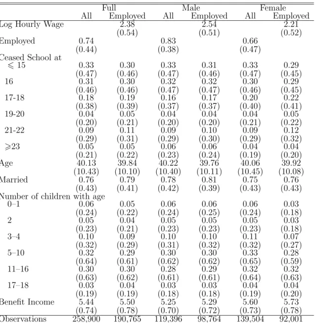
2.5.1 Data . . . 109
2.5.2 Empirical Specifications . . . 113
2.5.3 Model Parameters . . . 114
compositions . . . 118
2.5.5 Discussion . . . 127
2.6 Monte Carlo Simulation . . . 129
2.7 Conclusion . . . 132
2.8 Proofs of Section 2.2 . . . 133
2.8.1 Proof of Lemma 12 . . . 133
2.8.2 Proof of Theorem 2.1 . . . 134
2.9 Detailed Comparison with AB17 . . . 136
2.10 Model for Offered and Reservation Wages . . . 138
2.11 Notation . . . 139
2.12 Proofs of Section 2.4 . . . 139
2.12.1 Auxiliary Results . . . 140
2.12.2 Proof of Theorem 2.2 . . . 142
2.12.3 Proof of Theorem 2.3 . . . 144
2.13 Expressions of the Score and Expected Hessian . . . 145
2.13.1 Score . . . 145
2.13.2 Expected Hessian . . . 147
2.14 Supplement to “Distribution Regression with Sample Selection, with an Application to Wage Decompositions in the UK ” . . . 148
2.15 Influence Function . . . 149
2.16 Gradient and Hessian of Log-Likelihood Function . . . 171
2.16.1 Gradient based on analytical form . . . 172
2.16.2 Hessian based on analytical form . . . 173
2.16.3 Gradient and Hessian for First Stage . . . 174
3.1 Introduction . . . 177
3.2 An Iterative Estimation Algorithm . . . 180
3.2.1 Properties of Algorithm . . . 183
3.2.2 Model with Endogeneity . . . 184
3.3 Monte Carlo Simulations . . . 185
3.3.1 Pseudo Data Generating Process . . . 185
3.3.2 Variations in Parameters . . . 187
3.3.3 Results . . . 188
3.4 Empirical Example . . . 189
3.4.1 Health Plan Type Effects on Health Care Utilization . . . 189
3.4.2 Results . . . 190
3.5 Conclusions and Discussion . . . 191
3.6 Appendix A: Proof of Theorems and Corollary . . . 197
3.6.1 Proof of Theorem 1: . . . 197
3.6.2 Proof of Theorem 2: . . . 200
3.6.3 Proof of Corollary 1: . . . 202
3.7 Appendix B: Implementation of TSLSFECLUS Algorithm . . . 203
3.7.1 B.1. Implementation Steps . . . 203
3.7.2 B.2. Sample Call of TSLSFECLUS . . . 204
3.7.3 B.3. Clustering Standard Errors . . . 205
References 207
Curriculum Vitae 214
1.1 Summary Statistics . . . 21
1.2 Simulation Results: 95% Confidence Bands of Parameters . . . 55
2.1 Summary Statistics . . . 112
2.2 Properties of 95% Confidence Bands . . . 132
2.3 Estimates of Coefficients of the Employment Equation . . . 149
2.4 Employment rate decomposition between men and women . . . 149
3.1 Comparison of Programs . . . 193
3.2 Simulation Parameters for Two-way Fixed Effects Model . . . 193
3.3 Simulation Results . . . 194
3.4 Health Plan Type Effects on Health Care Utilization . . . 195
1·1 Estimates and 95% uniform confidence bands for the FE-DR coeffi-cients of log distance, religion, common language, common legal sys-tem, regional trade agreement and correlation. . . 23 1·2 Bias corrected estimates and 95% uniform confidence bands for the
latent and conditional distribution functions of the log volume of trade. 25 1·3 Estimates and 95% uniform confidence bands for the quantile effects
of log distance and common legal system on the latent and observed log volume of trade. . . 26 1·4 Estimates and 95% uniform confidence bands with pairwise clustering
dependence for the quantile effects of log distance and common legal system on the latent and observed log volume of trade. . . 27 1·5 Bias, standard deviation and root mean squared error for the
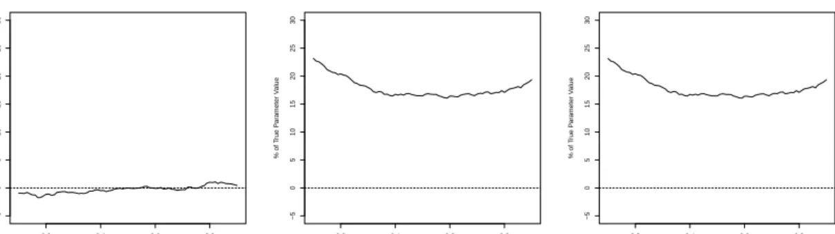
estima-tors of the FE-DR coefficients of log distance. . . 53 1·6 Bias, standard deviation and root mean squared error for the
estima-tors of the FE-DR coefficients of common legal system. . . 53 1·7 Bias, standard deviation and root mean squared error for the
estima-tors of the FE-DR coefficients of unobserved selection. . . 54
2·1 Trends in U.K. labor market 1978-2013 by gender: left panel reports the average of the log wage rate, the middle panel reports the 90-10 percentile spread of the log wage rate, and the right panel reports the employment rate . . . 113
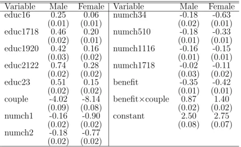
marital status in the outcome equation: specification 1 for men . . . . 116 2·3 Estimates and 95% confidence bands for coefficients of education and
marital status in the outcome equation: specification 1 for women . . 117 2·4 Estimates and 95% confidence bands for the selection sorting function:
specification 1 . . . 118 2·5 Estimates and 95% confidence bands for the selection sorting function:
specification 2 . . . 119 2·6 Estimates and 95% confidence bands for the selection sorting function:
specification 3 . . . 120 2·7 Estimates and 95% confidence bands for the selection sorting function:
specification 4 . . . 121 2·8 Estimates of the quantiles of observed and offered (latent) wages:
spec-ification 1 . . . 122 2·9 Estimates and 95% confidence bands for the quantiles of offered (latent)
wages and decomposition between women and men: specification 1 . 123 2·10 Estimates and 95% confidence bands for the quantiles of observed
wages and decomposition between men and women in specification 1 . . . 126 2·11 Estimates and 95% confidence bands for the quantiles of observed
wages and decomposition between first and second half of the sam-ple period for women in specification 1 . . . 127 2·12 Estimates and 95% confidence bands for the quantiles of observed
wages and decomposition between first and second half of the sam-ple period for men in specification 1 . . . 128
outcome equation . . . 131 2·14 Bias, SD and RMSE for the coefficient of the marital status indicator
in the outcome equation . . . 131 2·15 Bias, SD and RMSE for coefficient ρ(y) in the selection sorting equation131 2·16 Estimates and 95% confidence bands for coefficients of education and
marital status in the outcome equation: specification 2 for men . . . . 150 2·17 Estimates and 95% confidence bands for coefficients of education and
marital status in the outcome equation: specification 2 for women . . 151 2·18 Estimates and 95% confidence bands for coefficients of education and
marital status in the outcome equation: specification 3 for men . . . . 152 2·19 Estimates and 95% confidence bands for coefficients of education and
marital status in the outcome equation: specification 3 for women . . 153 2·20 Estimates and 95% confidence bands for coefficients of education and
marital status in the outcome equation: specification 4 for men . . . . 154 2·21 Estimates and 95% confidence bands for coefficients of education and
marital status in the outcome equation: specification 4 for women . . 155 2·22 Estimates and 95% confidence bands for coefficients of fertility in the
outcome equation: specification 1 for men . . . 156 2·23 Estimates and 95% confidence bands for coefficients of fertility in the
outcome equation: specification 1 for women . . . 157 2·24 Estimates and 95% confidence bands for coefficients of the selection
sorting function: specification 3 . . . 158 2·25 Estimates and 95% confidence bands for coefficients of the selection
sorting function: specification 4 . . . 159
offered (latent) wages: specification 1 . . . 160 2·27 Estimates and 95% confidence bands for the quantiles of observed and
offered (latent) wages: specification 1 . . . 160 2·28 Estimates and 95% confidence bands for the quantiles of observed and
offered (latent) wages and decomposition of offered wages between women and men: specification 2 . . . 161 2·29 Estimates and 95% confidence bands for the quantiles of observed and
offered (latent) wages and decomposition of offered wages between women and men: specification 3 . . . 161 2·30 Estimates and 95% confidence bands for the quantiles of observed and
offered (latent) wages and decomposition of offered wages between women and men: specification 4 . . . 161 2·31 Estimates and 95% confidence bands for decomposition between men
and women with aggregated selection effects in specification 1 . . . . 162 2·32 Estimates and 95% confidence bands for the quantiles of observed
wages and decomposition between men and women: (left) specifica-tion 2, (middle) specificaspecifica-tion 3, and (right) specificaspecifica-tion 4 . . . 162 2·33 Estimates and 95% confidence bands for the quantiles of observed
wages and decomposition between men and women with aggregated se-lection effect: (left) specification 2, (middle) specification 3, and (right) specification 4 . . . 163 2·34 Estimates and 95% confidence bands for components of wage
decom-position between women and men in specification 1 . . . 164 2·35 Estimates and 95% confidence bands for components of wage
decom-position between women and men in specification 2 . . . 165
position between women and men in specification 3 . . . 166 2·37 Estimates and 95% confidence bands for components of wage
decom-position between women and men in specification 4 . . . 167 2·38 Estimates and 95% confidence bands for components of wage
decom-position between first and second half of sample period for men in specification 1 . . . 168 2·39 Estimates and 95% confidence bands for components of wage
decom-position between first and second half of sample period for women in specification 1 . . . 169
3·1 Convergence of Estimates of Health Plan Type Effects on Health Care Utilization . . . 196
ABC . . . Analytical Bias Corrected CB . . . Confidence Bands
CDF . . . Cumulative Distribution Function CDHP . . . Consumer-Driven Health Plan COMP . . . Comprehensive
CPS . . . Current Population Survey DR . . . Distribution Regression
EPO . . . Exclusive Provider Organization FCLT . . . Functional Central Limit Theorem FE . . . Fixed-Effect
FOC . . . First Order Condition GDP . . . Gross Domestic Product
GMM . . . Generalized Method of Moments HDFE . . . High-Dimensional Fixed Effect HDHP . . . High-deductible Health Plan HMO . . . Health Maintenance Organization HSM . . . Heckman Selection Model
JBC . . . Jackknife Bias Corrected LGR . . . Local Gaussian Representation LSDV . . . Least Squares Dummy Vairble OLS . . . Ordinary Least Squares
PCP . . . Primary Care Physician PDF . . . Probability Density Function POS . . . Point of Service
PPO . . . Preferred Provider Organization QEF . . . Quantile Effect Function
QF . . . Quantile Function
RMSE . . . Root Mean Square Error RTA . . . Regional Trade Agreement
SBC . . . Split-Sample Jackknife Bias Corrected SD . . . Standard Deviation
SE . . . Standard Error
2SLS . . . Two-Stage Least Squares
Quantile Effects in a Sample Selection
Model for Network and Panel Data
Abstract
I develop a distribution regression model with sample selection for panel and network data. The model specifies a bivariate Gaussian distribution of the latent selection and outcome variables semiparametrically with function-valued parameters and un-observed effects. The unun-observed effects are included in the selection equation, out-come equation and selection sorting, allowing for very rich patterns of unobserved heterogeneity. I provide a two-step fixed-effect method to estimate the model param-eters and other functionals such as distributions and quantile effects. In addition, I derive analytical and Jackknife bias corrections to deal with the incidental parameter problem of the fixed-effect estimators. A multiplier bootstrap algorithm is adopted to construct confidence bands for uniform inference on the model parameters and func-tionals of interest. I apply this model to the gravity equation of trade network data between countries accounting for possibly endogenous zero trade decisions and unob-served country heterogeneity. The model credibly identifies positive and homogeneous effects of having a common legal system and negative effects of increasing pairwise distance on the latent trade volume that are heterogeneous across the distribution.
Keywords: Sample selection, distribution regression, heterogeneity, network, panel data, incidental parameter problem, fixed effects, uniform inference, gravity equation, bilateral
trade
JEL classification: C13, C14, C33, F12
Acknowledgements: I am grateful to my advisor Iv´an Fern´andez-Val for his
valu-able advice and support. I also thank professors Hiroaki Kaido, Randall Ellis and all participants in the Econometrics seminar and Econometrics reading group at Boston University for useful comments and insights. All errors belong to me.
1.1
Introduction
Sample selection is an important problem in empirical economics. It generally leads to biases in estimation when the sample selection process is related to the data gener-ating process of the variables of interest. The Heckman selection model (HSM), first introduced in Heckman (1974), is a popular solution that utilizes an auxiliary equa-tion to control for sample selecequa-tion. However, in addiequa-tion to parametric assumpequa-tions, HSM imposes strong homogeneity restrictions on the selection process and effect of covariates. Arellano and Bonhomme (2017a) and Chernozhukov et al. (2018a) pro-posed alternative models to relax these restrictions based on quantile regression and distribution regression, respectively. Both models are designed for cross-section data. I develop a distribution regression model with sample selection for network and panel data, which in addition to relaxing the homogeneity restrictions of the Heckman se-lection model, accounts for endogenous unobserved heterogeneity along each of the dimensions of the panel or network data.
The distribution regression model that I consider has three components: a selec-tion equaselec-tion, an outcome equaselec-tion, and a selecselec-tion sorting equaselec-tion that represents the relationship between the latent selection and outcome variables. The parameters of the outcome and selection sorting equations are function-valued over the support of the latent outcome, which can be continuous, discrete or mixed, and the selection
process can depend on covariates. Moreover, the availability of panel or network data allows me to include two-way unobserved effects in the three equations of the model to control for unobserved heterogeneity along the two dimensions of the data. These unobserved effects capture heterogeneity that might be related to the covariates. I show how to construct functionals of the model parameters such as actual and coun-terfactual distribution and quantile functions of the latent and observed outcome of interest, together with quantile and average effects.
I estimate the model using a two-step fixed-effect method that treats all the unob-served effects as parameters or fixed effects. The first step is a probit for the selection equation with two-way fixed effects. The second step contains multiple binary regres-sions with multidimensional two-way fixed effects and sample selection corrections to estimate the outcome and selection sorting equations. Functionals of the model parameters are estimated using the plug-in rule. The resulting estimators suffer from the incidental parameter problem because the estimating equations in the two steps are nonlinear and the dimension of the fixed effects increases with the number of observations.
I derive analytical and jackknife bias corrections to deal with the incidental param-eter problem following the recent large-T panel data literature (Arellano and Hahn,
2006; Fern´andez-Val and Weidner, 2018). To do so, I characterize the bias of
two-step fixed-effect distribution regression estimators with function-valued parameters and multidimensional two-way fixed effects. I find several sources for the bias in the estimators of the outcome and selection sorting equations: (1) randomness in the estimator of the fixed effects in the second step and the nonlinearity in these effects; (2) bias in the correction terms coming from the bias of the first step estimator and nonlinearity of the second step on the correction terms; and (3) correlation between the estimators of the fixed effects in the first and second steps. The last two sources
of bias are specific to the multi-step nature of the estimation procedure.
I show how to construct confidence bands to perform uniform inference on valued parameters and functionals. These bands cover the parameters or function-als uniformly over the region of interest with prespecified probability asymptoti-cally. They are formed as the point estimator plus and minus the critical value of a Kolmogorov-Smirnov type statistic times the standard errors. I adopt a multiplier bootstrap scheme to estimate the critical values. The multiplier bootstrap scheme is convenient because it avoids estimation of model parameters in each bootstrap repli-cation. Moreover, it does not require any bias correction as the distribution of the bootstrap draws is centered around the uncorrected fixed effects estimators. I rely on the influence functions of the parameters and functionals to estimate the standard errors. I start by assuming independence of the outcome along the two dimensions of the panel data conditional on the covariates and unobserved effects. Then I show how to relax this assumption topairwise clustering, a form of weak dependence that is common in network data. It allows the observations with symmetric indexes to be correlated based on some unobservables that are not captured by the unobserved effects. I show that pairwise clustering does not affect the estimation nor the bias corrections, but the inference method needs to be adjusted. The standard errors need to take into account the correlation between the symmetric observations and the weights in the multiplier bootstrap also need to be symmetric.
I apply the model to the gravity equation of international trade flows in 2013. The selection is whether there is any trade between two countries or not. Given non-zero trade, I estimate the effect of bilateral trade barriers on the volume trade. As inHelpman et al. (2008), I use the fixed cost to trade as an exclusion restriction, i.e., a variable that affects selection but not the latent outcome. A feasible measure for the fixed cost is based on regulation of firm entry. I construct the data set
from the bilateral trade data of Glick and Rose (2016), World Factbook of Central Intelligence Agency, and the updated firm regulation data collected by the World Bank. My measure of fixed cost is more complete than that inHelpman et al.(2008) due to recent collection of data. I find that the distance between two countries has smaller (less negative) effect on trade volume at the bottom than at the top of the distribution and that having a common legal system has homogeneous and significant positive effect on the latent and observed trade volume accounting for the potentially endogenous trade selection decision. I also uncover positive selection sorting at the bottom of the distribution of the trade volume and negative at the top.
Literature Review. The sample selection problem has a long history in
economet-rics. Classical references for cross-section data include Heckman (1974), Heckman
(1976), Heckman (1979), Lee (1982), Goldberger (1983), Amemiya (1985), Maddala
(1986), Heckman (1990) and Vella (1998). There is also previous work in
econo-metrics analyzing sample selection in panel data. This includes Hausman and Wise
(1979),Nijman and Verbeek(1992),Verbeek and Nijman (1992),Wooldridge(1995),
Rosholm and Smith (1996) andKyriazidou (1997). All these papers consider models
with finite-dimensional parameters and one-way unobserved effects.
The most closely related work to this paper includes Fern´andez-Val and Vella
(2011), Chernozhukov et al. (2018b) and Chernozhukov et al. (2018a). Fern´
andez-Val and Vella (2011) developed bias corrections for two-step fixed effects estimators
of finite dimensional parameters in models with one-way fixed effects. Chernozhukov
et al.(2018b) derived bias corrections for one-step fixed effects estimators of model
pa-rameters and related functionals in distribution regression models with two-way fixed effects without sample selection. Chernozhukov et al.(2018a) considered distribution regression models with sample selection, but without fixed effects. Relative to these papers I address the following challenges: (1) multidimensional unobserved effects,
(2) more complicated derivation of bias given the multi-step estimation methods, and (3) uniform validity of analytical bias corrections for function-valued parameters and functionals.
Outline. Section 1.2 introduces the distribution regression model accounting for
sample selection and unobserved effects for network and panel data, and describes the model parameters and other functionals of interest. Section 1.3 shows the esti-mation procedure, incidental parameter problem and bias corrections, and uniform inference for the function-valued parameters and functionals. Section 1.4 reports the results of my empirical application of this model to the gravity equation of bilateral trade. Section 1.5 provides asymptotic theory including the analytical derivation of the bias, development of functional central limit theorems for the uncorrected and bias corrected estimators of the parameters and functionals, and the validity of the multiplier bootstrap inference, under the setting of one-way fixed effect. Section 1.6 demonstrates the Monte Carlo simulation calibrated to the application and Section 1.7 concludes. The proofs of the main results are given in the Appendix.
1.2
Model
I follow the literature by modeling the selection process using two latent variables. Let yij∗ be the latent outcome variable and d∗ij be the latent selection variable. Let also zij be adz-vector of observed covariates,xij be a subvector ofzij, and ui and vj
be two vectors of unobserved effects. I assume that the joint distribution of yij∗ and
d∗ij conditional on zij, ui and vj follow the bivariate distribution regression model:
Fy∗ ij,d∗ij(y,0|zij, ui, vj) = Φ2(−(x 0 ijβ(y)+u 0 iα2(y)+v 0 jγ2(y)),−(z 0 ijπ+u 0 iα1+v 0 jγ1);ρij(y)), (1.2.1) where Φ2 is the cumulative distribution function of the standard bivariate normal
distribution, ρij(y) = tanh(x0ijδ(y) +u 0
iα3(y) +vj0γ3(y))1 is the correlation coefficient
embedded in the joint distribution, y 7→ θ(y) := (β(y), δ(y)) are the function-valued parameters of interest, yij∗ is a scalar response variable with region of interest Y, which can be continuous, discrete or mixed,zij = (xij, bij) where bij are the excluded
covariates, and (α1, γ1, α2(y), γ2(y), α3(y), γ3(y)) is a full set of parameters of the
unobserved effects that account for unobserved heterogeneity. The strict exclusion restriction assumption xij ⊂ zij is a necessary assumption for point identification of
the model (see Chernozhukov et al., 2018a).
Here the minus signs in front of the first two indexes serve to facilitate interpre-tation. In other words, a positive parameter β(y) in (1.2.1) implies positive effects of covariatesxij onyij∗ and a positive parameter πindicates positive effects of covariates
on the latent selection (see Remark 1.2.1). I only need to model the latent selection variable at d = 0 because I can only observe whether d∗ij > 0. In fact the observed variables are
dij = 1(d∗ij >0) (1.2.2) yij = y∗ij if dij = 1, (i, j)∈ D, (1.2.3)
where dij is the selection indicator, yij is the observed outcome that corresponds to y∗ij if dij equals 1 and otherwise its value is missing.
Define α2i(y) := u0iα2(y) and γ2j(y) := vj0γ2(y) as the unobserved effects in the
outcome equation. I use the same notation in the selection and selection sorting equations to obtain α1i, γ1j, α3i(y) and γ3j(y). The set of observationsD is a subset
of the full range of the indexes, i.e. D ⊆ D¯ := {(i, j) | i = 1, . . . , I;j = 1, . . . , J}, whereI and J are the dimensions of the panel. The number of observations denoted byn =|D|.
1Any reparametrization that maps from
Model (1.2.1) - (1.2.3) allows for heterogeneity in the effects of covariates, selec-tion sorting and unobserved effects across the distribuselec-tion of the outcome variable, together with the unobserved effects along the dimensions of the panel data. These unobserved effects capture heterogeneity that might be correlated with the covariates. For example, in the empirical application of Section 1.4, I use trade data where i
and j index countries as exporters and importers,I =J, and observations withi=j
are missing because trade of a country with itself can not be observed. The selector
dij indicates whether a trade flow occurs from countryito countryj and the outcome yij is the logarithm of the trade volume from country i to country j. The covariates xij include gravity variables such as the logarithm of distance between country i and j, and the excluded variable bij is a trade barrier that affects fixed trade costs but
does not affect variable trade costs. Following Anderson and Van Wincoop (2003), I include unobserved importer and exporter country effects in all the equations of the model. These fixed effects control for other country specific characteristics that may have an impact on the trade occurrence, trade volume and the correlation between the unobservables that determine occurrence and volume. For example, these country-level characteristics may be GDP, tariffs, population, institutions, infrastructures or natural resources.
Model (1.2.1) - (1.2.3) specifies the joint distribution of the latent outcome and latent selection. By looking at the marginal distribution of each latent variable, the model has a representation with a two-step structure that is comparable to the classical HSM
Selection Equation:
Outcome Equation: P(yij∗ 6y|zij, ui, vj) =Fy∗ ij(y |zij, ui, vj) = Φ −(x 0 ijβ(y) +α2i(y) +γ2j(y)) ,
where the Selection Equation is a panel probit model for the probability of being observed dij = 1 conditional on covariates and unobserved effects. In the trade
application, the Selection Equation specifies the probability of the event that trade occurs between countries using a probit model and the Outcome Equation specifies the probability of trade volume being less than a certain threshold y. Sample selection bias arises because the distributions of yij and y∗ij are not the same, i.e. Fyij(y | zij, ui, vj)6=Fy∗ij(y |zij, ui, vj), since Fy∗ij(y |zij, ui, vj) =Fyij∗(y|zij, ui, vj, dij = 1) = Φ2(−(x 0 ijβ(y) +α2i(y) +γ2j(y)), z0ijπ+α1i+γ1j;−tanh(x0ijδ(y) +α3i(y) +γ3j(y))) Φ(z0 ijπ+α1i+γ1j) .
Remark 1.2.1 (HSM with Unobserved Effects). A panel version of the HSM with
unobserved effects in the selection and outcome equations is a special case of (1.2.1). Thus, consider the model
yij∗ = x0ijβ+α2i+γ2j +σ2,ij
d∗ij = zij0 π+α1i+γ1i+1,ij
where (1,ij, 2,ij) are jointly standard bivariate normal with correlation ρ, dij =
1(d∗ij > 0) and yij = y∗ij if dij = 1. The conditional joint distribution of yij∗ and
d∗ij is Fy∗ ij,d∗ij(y,0|zij) = Φ2 y−(x0 ijβ+α2i+γ2j) σ ,−(z 0 ijπ+α1i+γ1i);ρ .
This is a special case of model (1.2.1) with the intercept β1(y) = (β1 −y)/σ, slopes
β−1(y) =β−1/σ, unobserved effects α2i(y) =α2i/σ and γ2j(y) =γ2j/σ, and selection
1.2.1 Counterfactual distributions and other functionals
In addition to model parameters, we might be interested in other estimands including counterfactual distributions, quantile functions, quantile effect functions and average effects. In the trade application, the average effect of distance on trade volume, or the median effect of having the same legal system on trade volume are potentially interesting. Let xij = (tij, rij0 )
0 where t
ij is the treatment of interest and rij are
controls. Then, the treatment effect on the distribution of yij∗ is the difference of the distribution functions resulting from switching tij from a level t0ij to t1ij holding the
other covariates rij and unobserved effects constant. Denote xij,k = (tkij, r 0
ij)
0 and
zij,k= (tkij, r0ij, bij)0 for k ∈ {0,1}, where the treatment level tkij may vary by the type
of treatment variable tij2. The counterfactual marginal distributions of the latent
outcome y∗ij and observed outcomeyij fortij =tkij, k ∈ {0,1} are correspondingly,
Fk∗(y) = 1 n
X
(i,j)∈D
Φ(−(x0ij,kβ(y) +α2i(y) +γ2j(y))),
Fk(y) =
P
(i,j)∈DΦ2 −(x0ij,kβ(y) +α2i(y) +γ2j(y)),z0ij,kπ+α1i+γ1j;−ρ(x0ij,kδ(y), α3i(y) +γ3j(y))
P
(i,j)∈DΦ(z0ij,kπ+α1i+γ1j)
.
Following Chernozhukov et al. (2018b), I marginalize zij using the empirical
distri-bution to construct the counterfactual distridistri-butions. Note that for the distridistri-butions of yij, the selection process varies with the treatment level. The selection
mecha-nism endogenously affects the empirical distribution of the covariates for the selected population, which leads to the conditional form of the distribution function.
In the trade application, the treatment variables of interest can be any country-pair trade barrier. I choose the log distance between two countries and whether the two countries have a common legal system as the treatment variables in Section 1.4.
2Types of treatment variable and the corresponding treatment levels are binary, t0
ij = 0 and
t1
ij = 1; continuous, t0ij =tij and tij1 = tij+d, d= 1 orSD(tij); and the logarithm of continuous treatment,t0ij =tij andt1ij=tij+ log 2.
The counterfactual distributions correspond to varying distance or common legal sys-tem between two different treatment levels. For example, Fk∗(y) is the counterfactual distribution of the latent trade volume when the distance or common legal system is at the treatment level k. The latent trade volume can be interpreted as a proposed volume of trade from country i to country j or the trade volume specified by a con-tract under discussion between countyi and j. It shows the fictional volume of trade without fixed costs. On the other hand, Fk(y) shows the counterfactual distribution
of the trade volume that we would observe accounting for the potential endogenous change of the trade decision due to the change of treatment. Both types of outcomes might be of interest to policy makers because they reveal information at different steps during the trade decision process. The distribution of latent trade volume il-lustrates how the treatment affects the prior-decision of trade volume without any fixed cost, whereas the distribution of observed trade volume takes into account the decision process and reflects possible effects on the posterior-decision of trade volume. Quantile functions (QF) are left inverses of distribution functions and the differ-ence of QFs taking the treatment variable at the two levels considered is the quantile effect function (QEF). Take the latentyij∗ for example,
Q∗k(τ) =Fk∗←(τ) := inf{y∈ Y :Fk∗(y)>τ} ∧sup{y∈ Y}, k∈ {0,1},
∆∗(τ) =Q∗1(τ)−Q∗0(τ),
where τ ∈ (0,1). The average effect can also be obtained by obtaining the counter-factual averages from the distribution function,
M∗k = Z
[1(y>0)−Fk∗(y)]dy, k ∈ {0,1},
∆∗ =M∗1− M∗0.
procedure replacing the distribution functionsFk∗(y) withFk(y). The above QEF and
average effect have causal interpretation under some standard unconfoundedness or independence assumptions for panel data, conditional on both the observed control variables and the unobserved effects.
1.3
Estimation and Uniform Inference
I estimate the model parameters using a two-step method similar to the Heckman two-step method. The two-way unobserved effects are included in both steps and treated as parameters or fixed effects. In a third step, I estimate the functionals via the plug-in rule. Denote the indicators of observed response being lower than a specific threshold asgij(y) := 1{yij 6y} fory∈Y¯, a finite grid of points covering Y, gij = {gij(y) : y ∈ Y}¯ , and wij ((i, j) ∈ D) are the data observations including the
covariates and the indicators for both selection and outcome, i.e. wij = (zij, dij, gij).
Let the three vectors of fixed effects be correspondinglyε1 = (α11, . . . , α1I, γ11, . . . , γ1J)0,ε2(y) = (α21(y), . . . , α2I(y), γ21(y), . . . , γ2J(y))
0
, andε3(y) = (α31(y), . . . , α3I(y), γ31(y), . . . , γ3J(y))
0
, and the three indexes be µ1ij = z0ijπ + α1i + γ1j, µ2ij(y) = x0ijβ(y) +α2i(y) +γ2j(y) and µ3ij(y) = x0ijδ(y) +α3i(y) +γ3j(y).
The conditional likelihood of (dij, gij(y)) given the selection parameter π, the
outcome parameters of interestθ(y) = (β(y), δ(y)), the covariateszij and the additive
fixed effects, is identical to the bivariate probit for (dij, gij(y)) with fixed effects,
Ly(wij;π, θ(y), ε1, ε2(y), ε3(y)) = [1−Φ(µ1ij)] 1−dij×
Φ2(µ1ij,−µ2ij(y);−tanh(µ3ij(y)))dijgij(y) ×Φ2(µ1ij, µ2ij(y); tanh(µ3ij(y)))dij(1−gij(y)). I maximize the average log-likelihood with respect to the parameters and fixed effects. The following procedure summarizes the estimation of the parameters and functionals of interest:
Estimation Procedure.
Step 1: Panel probit for Selection Equation
(bπ,ε1b) = arg max π∈Rdz,ε1∈RI+J X (i,j)∈D `1(wij;π, ε1), `1(wij;π, ε1) := dijlog Φ(µ1ij) + (1−dij) log Φ(−µ1ij). (1.3.1)
Step 2: Panel distribution regression with selection for Outcome Equa-tion (bθ(y),ε2b(y),ε3b(y)) = arg max θ∈Rdx+dδ;ε2,ε3∈RI+J X (i,j)∈D `y2(wij,µ1b ij;θ, ε2, ε3), `y2(wij, µ1ij;θ(y), ε2(y), ε3(y)) := dijgij(y) log Φ2(µ1ij,−µ2ij(y);−tanh(µ3ij(y))) +dij(1−gij(y)) log Φ2(µ1ij, µ2ij(y); tanh(µ3ij(y))), b µ1ij =zij0 bπ+αb1i+bγ1j. (1.3.2)
Step 3: Plug-in estimation for QF, QEF and average effect
b Fk∗(y) = 1 n X (i,j)∈D Φ(−(x0ij,kβb(y) +αb2i(y) +bγ2j(y))), b Fk(y) = P (i,j)∈DΦ2(−(x0ij,kβb(y) + b α2i(y) +bγ2j(y)),µb1ij,k;−ρbij,k(y)) P (i,j)∈DΦ(µb1ij,k) , y∈Y¯, b Q∗k(τ) =Fbk∗←(τ)∧sup{y∈ Y}, Qbk(τ) =Fbk←(τ)∧sup{y∈ Y}, τ ∈(0,1), k ∈ {0,1}, b ∆∗(τ) =Qb∗1(τ)−Qb∗0(τ), ∆(b τ) =Qb1(τ)−Qb0(τ), τ ∈(0,1), c M∗k = Z [1(y>0)−Fbk∗(y)]dy, Mck = Z [1(y>0)−Fbk(y)]dy, k ∈ {0,1}, b ∆∗ =Mc∗1−Mc0∗, ∆ =b Mc1−Mc0. (1.3.3)
1.3.1 Incidental parameter problem
Fixed-effect (FE) estimators in nonlinear panel models suffer from the incidental pa-rameter problem. Incidental papa-rameters are nuisance papa-rameters whose dimension grows with the sample size. Neyman and Scott (1948) showed that the maximum
likelihood estimators can be asymptotically biased in models with incidental param-eters and the order of bias is approximately the ratio of the number of paramparam-eters to the number of observations (see Fern´andez-Val and Weidner, 2018). Let θb(y) be a generic function-valued multi-step FE estimator of the parameters of interest. The incidental parameter problem arises because θb(y) depends on the sample estimates of the unobserved effects and is contaminated by their randomness. The following functional central limit theorem is established in Section 1.5 with one-way fixed effect for both the fixed-effect distribution regression with selection (FE-DR-Selection) esti-mators of model parameters in Step 2 and the FE estiesti-mators of distribution functions in Step 3, √ n b θ(y)−θ0(y)− I nB (θ)(y)− J nD (θ)(y) Z(θ)(y), (1.3.4)
where Z(θ)(y) is the zero-mean Gaussian processes indexed by y ∈ Y, B(θ)(y) and D(θ)(y) are the bias terms, and denotes weak convergence
Chernozhukov et al. (2018b) develops the functional central limit theorems for
the FE estimators in one-step logit distribution regression. For the point-valued estimator in two-step models with individual fixed effect, Fern´andez-Val and Vella
(2011) provides the corresponding asymptotic theory. By the multi-step nature of the estimation procedure, more types of randomness are taken into account to derive the expression of bias terms in (1.3.4). The sources of bias in (1.3.4) include the estimation of fixed effects in first step via control functions and the correlation of fixed effects in different steps, in addition to the typical within-step estimation of fixed effects. The distributions of the latent and observed outcomes are analogous to average partial effects. My goal is to characterize the bias and develop the bias correction methods for the multi-step FE estimator of function-valued parameter and the functionals such as distributions.
1.3.2 Bias corrections Analytical bias correction
Let Bb(θ)(y) and Db(θ)(y) be consistent estimators of B(θ)(y) and D(θ)(y) described in (1.3.4) respectively, then the analytical bias corrected (ABC) estimators can be formed as e θABC(y) =θb(y)− I nBb (θ)(y)− J nDb (θ)(y). (1.3.5)
The correction removes the first order asymptotic bias provided thatI/√n(Bb(θ)(y)−
B(θ)(y))−→p 0 andJ/√n( b D(θ)(y)−D(θ)(y))−→p 0 uniformly in y∈ Y because √ n e θABC(y)−θ0(y) =√n b θ(y)−θ0(y)− I nB (θ) (y)− J nD (θ) (y) −√I n b B(θ)(y)−B(θ)(y)− √J n b D(θ)(y)−D(θ)(y) Z(θ)(y). (1.3.6) The ABC estimators of thedistribution functions are constructed similarly to (1.3.5). For example for the marginal distribution of latent outcome3,
e Fk,ABC∗ (y) =Fbk∗(y)− I nBb (F∗) k (y)− J nDb (F∗) k (y), (1.3.7) where Bb (F∗) k (y) and Db (F∗)
k (y) are consistent estimators of asymptotic bias that
cor-responds to the distribution function of latent outcome Bk(F∗)(y) and Dk(F∗)(y). Bias corrected FE estimators of other estimands are formed via the plug-in rule. For exam-ple for QF Q∗k(τ), Qe∗k(τ) =Fek,ABC∗← (τ)∧sup{y ∈ Y}. The analytical bias corrections for other functionals relevant to the observed outcome are analogous. The bias cor-rected estimator of distribution functions is also used as the basis for inference in the
3Note that if the bias corrected estimator y 7→
e
Fk,ABC∗ (y) is non-monotone on Y, it can be monotonized by simply sorting the values of function in a nondecreasing order (seeChernozhukov et al.,2009) for detailed properties of monotonization.
empirical implementation.
Jackknife bias correction
There are two main Jackknife bias correction methods applicable to my model. Fol-lowingDhaene and Jochmans(2015) andFern´andez-Val and Weidner(2016), the first correction is based on the idea of splitting the panel into two half panels in which the bias is double that in the original panel. In the case of two-way effects, splitting the panel along each of the dimensions doubles the corresponding bias term while keep-ing the other bias term constant. The split-sample Jackknife bias corrected (SBC) estimator is constructed as e θSBC(y) := 3bθI,J(y)−θeI,J/2(y)−θeI/2,J(y), (1.3.8) where θeI,J/2(y) := 12 h b θI,{j6dJ/2e}(y) +θbI,{j6bJ/2+1c}(y) i
is the average of estimators using each of the half samples split along dimension j, dwe denotes the smallest integer that is greater thanw, bwcdenotes the largest integer that is smaller thanw, and θeI/2,J(y) is defined by splitting along dimension i instead. The SBC estimator mitigates the asymptotic bias because θeI,J/2(y)−θbI,J(y)'B(θ)(y)/J and θeI/2,J(y)− b
θI,J(y)'D(θ)(y)/I.
In the trade application with the symmetric panel or network data, the importers and exporters contain the identical set of countries. Another feasible Jackknife method for bias correction fits in this circumstance is the leave-one-country-out Jack-knife bias corrected (JBC) estimates (see Cruz-Gonzalez et al., 2016). Given that
I =J, the JBC estimator is
e
θJ BC(y) :=Iθb(y)−(I −1)¯θ(y), (1.3.9) where ¯θ(y) =I−1PI
that excludes observations associated with country i as either importer or exporter. For example, when country i represents the United States, θb−i(y) is the estimator
after eliminating the trade records of the United States exporting to/importing from other countries. θeJ BC(y) is asymptotically unbiased because (I −1)(¯θ(y)−θb(y)) '
B(θ)(y)/I+D(θ)(y)/I.
1.3.3 Uniform inference
Based on the asymptotic property for ABC estimator (1.3.6), one can construct point-wise and uniform confidence bands (CB) for the function-valued parameters of inter-est y 7→ θ(y) on Y. For a given p ∈ (0,1), a pointwise p-confidence interval uses the (1−p/2)-quantile of a standard normal distribution as the critical value. Let
B ⊆ {1, . . . , dβ +dδ} be the set of indexes for the coefficients of interest, where dβ
and dδ denote the dimensions of β(y) and δ(y) respectively. To construct a uniform
(asymptotic) p-confidence band CBp(θl(y)) for θl(y), l ∈ B such that the parameters θl(y) is covered uniformly with probability p,
P r[θl(y)∈CBp(θl(y)),∀y∈ Y]→p,
the Kolmogorov-Smirnov type critical values are used instead. For example, a joint uniform p-confidence bands for a vector of functions {θl(y) : l ∈ B, y ∈ Y} is CBp(θ(y)) = {[eθl(y)±t
(θ)
B,Y(p)bσθl(y)] : l ∈ B, y ∈ Y}. The critical value t
(θ)
B,Y(p) is
the p-quantile of the maximal t-statistic over B and Y and σbθl(y) is the standard
error of θel(y).
The normality of counterfactual distributions is established in Section 1.5 and infers analogously the constructions of pointwise and uniform p-confidence bands for
y 7→ Fk∗(y) and y 7→ Fk(y) on Y. The uniform confidence bands are constructed
t(K,YF∗)(p) and t(K,YF)(p). The confidence bands for the corresponding quantile functions and effects can be developed from the confidence bands for the distribution functions using the transformation method in Chernozhukov et al. (2016).
I utilize the influence functions of the parameters and distribution functions to compute the standard errors and the critical values. An influence function shows the sensitivity of the estimator with respect to the sample points and the expressions of influence functions are displayed in Section 1.5.5. The standard errors are constructed in (1.5.19) for parameters, and in (1.5.20) and (1.5.21) for distribution functions, whereψ2yij,ϕ∗yij and ϕyij are the influence functions respectively. To obtain the critical values of the maximalt-statisticsbt
(θ)
B,Y¯(p),bt
(F∗)
K,Y¯(p) andbt
(F)
K,Y¯(p), I propose the following
multiplier bootstrap algorithm.
Algorithm 1 (Multiplier Bootstrap). Let Y¯ be a finite grid covering the support Y.
(1) Draw the i.i.d standard normal multipliers {ωmij : (i, j) ∈ D} and normalize
them to have zero mean as a finite sample adjustment,
ωijm =ωeijm− X
(i,j)∈D
e
ωijm/n, eωmij i.i.d∼ N(0,1).
(2) For each y∈Y¯, obtain the bootstrap replication of the estimators
b θm(y) =θb(y) +n−1 X (i,j)∈D ωijmψ2yij(eπ,εe1,bθ(y), b ε2(y)), b Fk∗m(y) =Fbk∗(y) +n−1 X (i,j)∈D ωijmϕ∗yij(eπ,εe1,bθ(y), b ε2(y)), b Fkm(y) =Fbk(y) +n−1 X (i,j)∈D ωijmϕyij(eπ,eε1,θb(y), b ε2(y)), k ∈ K.
(3) Construct the bootstrap realization of the maximal t-statistics, where the
stan-dard errors σbθl(y), σbFk∗(y) and bσFk(y) are defined in (1.5.19), (1.5.20) and
(1.5.21) respectively t(B,θ)Y¯,m= max y∈Y¯,l∈B |θblm(y)−θbl(y)| b σθl(y) ,
t(K,FY∗¯),m= max y∈Y¯,k∈K |Fbk∗m(y)−Fbk∗(y)| b σF∗ k(y) , t(K,FY)¯,m= max y∈Y¯,k∈K |Fbkm(y)−Fbk(y)| b σFk(y)
(4) Repeat steps (1)-(3)M times and index the bootstrap draws bym ∈ {1, . . . , M}.
In the numerical examples I set M = 2004.
(5) Obtain the bootstrap estimators of the critical values as
bt (θ) B,Y¯(p) = p−quantile of {t (θ),m B,Y¯ : 16m6M}, b t(K,FY∗¯)(p) = p−quantile of {t(K,FY∗¯),m: 16m6M}, bt (F) K,Y¯(p) = p−quantile of {t (F),m K,Y¯ : 16m 6M}.
Pairwise Clustering. The default uniform inference assumes thatyij is independent
over i and j conditional on the covariates and unobserved effects. This assumption can be relaxed to account for some forms of weak dependence. In the application to the network data, a particular form of weak dependence ispairwise clustering or
reci-procity. The symmetric observations indexed by (i, j) and (j, i) might be correlated
due to some unobservables that are not captured by the unobserved effects. For trade network, these unobservables might be distributional channels between two countries or the exchange of bidirectional trade contracts.
Pairwise clustering does not affect estimation nor bias corrections, but the con-struction of standard errors and critical values. The standard errors are now obtained from (1.5.22), (1.5.23) and (1.5.24). The modified multiplier bootstrap algorithm in the circumstance of pairwise clustering is as follows.
Algorithm 2 (Multiplier Bootstrap with Pairwise Clustering). LetY¯be a finite grid
covering the support Y.
4One can set instead M = 199 for more explicit definition of p-quantile, yet M = 199 and M = 200 are equivalent in theory.
(1) Draw the i.i.d. standard normal multipliers {ωem
ij : (i, j) ∈ D, i 6 j}, assign
ωm
ji =ωijm and normalize them to have zero mean as a finite sample adjustment,
ωmij =ωemij − X
(i,j)∈D
e
ωijm/n, ωeijm i.i.d∼ N(0,1), i6j.
(2) For each y∈Y¯, obtain the bootstrap replications of the estimators
b θm(y) =θb(y) +n−1 X (i,j)∈D ωijmψ2yij(eπ,ε1,e bθ(y),ε2b(y)), b Fk∗m(y) =Fbk∗(y) +n−1 X (i,j)∈D ωijmϕ∗yij(eπ,εe1,bθ(y), b ε2(y)), b Fkm(y) =Fbk(y) +n−1 X (i,j)∈D ωijmϕyij(eπ,eε1,θb(y), b ε2(y)), k ∈ K.
(3) Construct the bootstrap realization of the maximalt-statistic wherebσθl(y), bσFk∗(y)
and bσFk(y) are defined in (1.5.19), (1.5.20) and (1.5.21) respectively
t(B,θ)Y¯,m= max y∈Y¯,l∈B |θblm(y)−θbl(y)| b σθl(y) , t(K,FY∗¯),m= max y∈Y¯,k∈K |Fbk∗m(y)−Fbk∗(y)| b σF∗ k(y) , t(K,FY)¯,m= max y∈Y¯,k∈K |Fbkm(y)−Fbk(y)| b σFk(y)
(4) Repeat steps (1)-(3)M times and index the bootstrap draws bym ∈ {1, . . . , M}.
In the numerical examples I set M = 200.
(5) Obtain the bootstrap estimators of the critical values as
bt (θ) B,Y¯(p) = p−quantile of {t (θ),m B,Y¯ : 16m6M}, b t(K,FY∗¯)(p) = p−quantile of {t (F∗),m K,Y¯ : 16m6M}, bt (F) K,Y¯(p) = p−quantile of {t (F),m K,Y¯ : 16m 6M}.
The clustered multiplier bootstrap preserves the dependence in the symmetric pairs (i, j) and (j, i) by assigning the same multiplier to each of these pairs.
1.4
Empirical Study
I apply the model to estimate gravity equations for directed bilateral trade between countries. The data are from Glick and Rose (2016), World Factbook of CIA and World Bank “Doing Business” project. These data sets contain information on bi-lateral trade flows and trade barriers for 176 countries in 20135. The data set is composed of network data where both iand j index countries as senders (exporters) and receivers (importers), and therefore I = J = 176. The outcome variable yij is
the logarithm of the bilateral trade volume from country i to country j in million US dollars. The selection variable dij indicates if the trade volume is positive. The
exogenous covariates xij include determinants of bilateral trade flows such as the
logarithm of the distance in kilometers between country i’s capital and country j’s capital, product of religion percentages in both countries i and j and indicators for common border, language, legal system, currency union, colonial relationship and regional trade agreement (RTA). The excluded covariate bij is a measure of common
ease of firm entry with scale [0,1] that is the product of regulation ranks of both countries i and j obtained from the World Bank “Doing Business” project.
Follow-ing Harrigan (1994) and Anderson and Van Wincoop (2003), I include unobserved
importer and exporter country effects to control for other country specific character-istics that may affect trade such as GDP, culture, tariffs, population, institutions, infrastructures or natural resources. These characteristics may affect differently the imports and exports of each country and be arbitrarily related with the observed covariates.
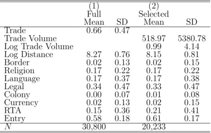
Table 1.1 reports descriptive statistics of the variables used in the analysis. There are 176×175 = 30,800 observations corresponding to different pairs of importer and 5Belgium and Luxembourg are combined as one observation. The term “country” is used here
for convenience and the trade partners include countries, regions, colonies, territories and overseas departments. United Kingdom, Germany and Japan are dropped because they imported from and/or exported to all other countries in my data set.
Table 1.1: Summary Statistics (1) (2) Full Selected Mean SD Mean SD Trade 0.66 0.47 Trade Volume 518.97 5380.78 Log Trade Volume 0.99 4.14 Log Distance 8.27 0.76 8.15 0.81 Border 0.02 0.13 0.02 0.15 Religion 0.17 0.22 0.17 0.22 Language 0.17 0.37 0.17 0.38 Legal 0.34 0.47 0.33 0.47 Colony 0.00 0.07 0.01 0.08 Currency 0.02 0.13 0.02 0.15 RTA 0.15 0.36 0.21 0.41 Entry 0.58 0.18 0.61 0.17 N 30,800 20,233
exporter. The observations with i = j are missing because the trade flow from a country to itself is neglected by nature, as opposed to the selection process. The
Trade variable is an indicator for positive volume of trade and serves as the observed
selection indicator. There are 34% of the country pairs with zero trade flows. The variableTrade Volume shows high skewness and thick upper tail by the fact that it is bounded below by 0 and by comparing the large standard deviation with the mean. This feature also induces distributional methods introduced in the model setting, because a large proportion of information congregates at the high quantiles.
Previous nonlinear parametric models in the international trade literature include Poisson, Negative Binomial and Tobit models that are chosen to deal with the large number of zeros in the volume of trade (see e.g. Eaton and Kortum, 2001; Silva and
Tenreyro,2006).6 These models impose parametric assumptions and the homogeneity
in the effects of covariates and model parameters. Chernozhukov et al. (2018b) relax these restrictions by specifying a logit DR model with fixed effects to explain the mass point at zero. In their model, the observations with zero trade volume are generated 6For a comprehensive survey on international trade models using gravity equation, (seeHead and
by the same process as other positive thresholds with locally adjusted parameters. In contrast to their model, I return to the Heckman selection fashion for an auxiliary endogenous sample selection process to generate observations with zero trade volume. Moreover, instead of a univariate distribution for the trade volumes including zero, I specify the bivariate distribution jointly for the latent selection for non-zero trades and the latent trade volume. I allow for additional covariates such as measures of fixed cost of trade to affect the trade decision. Analogous to the Heckman selection model (HSM), my model gives insights about the trade decision mechanism where the potential aggregate trade volumes are proposed before making the decision on whether the proposed trade is executed or not.
Helpman et al. (2008) discussed the feasibility of using the HSM for the positive
trade flows. The ideal excluded variable is a measure of fixed costs to the bilateral trade between countries that does not affect the variable cost of trade. Following
Helpman et al.(2008), I construct this variable as an aggregate country-level measure
on the regulatory costs of firm entry, which is magnified when both the importing and exporting countries have high regulatory frictions. By definition, the measure of regulation of firm entry is valid as an excluded variable because it affects the firm-level fixed rather than variable costs to trade. This instrument affects the selection process and the observed trade volume through the extensive margin. However, due to limited accessibility of regulation data at the time, the sample in Helpman et al.
(2008) for Heckman selection analysis suffers from a large truncation of observations using the regulation variable as the instrument. As the World Bank project of “Doing Business” continued since first introduced by Djankov et al. (2002), the regulation data has enriched and provided a reliable excluded variable for my model.
Figure 1·1 reports the estimates and the 95% uniform confidence bands for the FE-DR coefficients of log distance, religion, common language, common legal system
−6 −4 −2 0 2 4 6 −1.4 −1.2 −1.0 −0.8 −0.6 Log Distance
Log Volume of Trade
DR Coeff uncorrected ABC 95% CB Heckman −6 −4 −2 0 2 4 6 −1.0 −0.5 0.0 0.5 1.0 Religion
Log Volume of Trade
DR Coeff uncorrected ABC 95% CB Heckman −6 −4 −2 0 2 4 6 −0.6 −0.4 −0.2 0.0 0.2 0.4 0.6 Language
Log Volume of Trade
DR Coeff uncorrected ABC 95% CB Heckman −6 −4 −2 0 2 4 6 −0.2 0.0 0.2 0.4 0.6 Legal
Log Volume of Trade
DR Coeff uncorrected ABC 95% CB Heckman −6 −4 −2 0 2 4 6 −0.2 0.0 0.2 0.4 0.6 RTA
Log Volume of Trade
DR Coeff uncorrected ABC 95% CB Heckman −6 −4 −2 0 2 4 6 −1.0 −0.5 0.0 0.5 1.0 Rho
Log Volume of Trade
DR Coeff
uncorrected ABC 95% CB Heckman
Figure 1·1: Estimates and 95% uniform confidence bands for the
FE-DR coefficients of log distance, religion, common language, common legal system, regional trade agreement and correlation.
and regional trade agreement accounting for sample selection as well as the correlation between selection and outcome equations. I plot the uncorrected and ABC estimates defined in (1.3.2) and (1.3.5) against the quantile indexes of the log trade volume. The 95% uniform confidence bands centered at the ABC estimates are obtained from Algorithm 1 in Section 1.3.3 with 200 bootstrap replications and zero-mean standard normal multipliers. The constant estimates using the HSM are plotted in dotted line for reference. As predicted by the theory in Section 1.5, the differences between the uncorrected and ABC estimates are of the same magnitude as the band widths. For the coefficients of log distance, common legal system and regional trade agreement, the highest estimated bias happens at the upper quantiles, whereas for the other coefficients the bias correction is minor except at the extreme quantiles. The
inter-pretation of the parameters of the outcome equation are analogous to the parameters in a standard probit/logit model. The model parameters are proportional to the partial effects and therefore their ratios and signs can be interpreted. The signs of the FE-DR coefficients indicate that increasing the distance between two countries has a negative effect on the (latent) log volume of trade, and having a more common religious composition, sharing the same language, having a common legal system and participating in the same regional trade agreement all have a positive effect. The effects of log distance are significantly different from the Heckman estimate. The trade flows display positive selection at the bottom of distribution and insignificant selection at the top. This indicates that there is little unobserved sorting effect on the substantial potential trades through selection process and thus reveals an inertia. The heterogeneity in the selection effects is not captured by the HSM.
Figures 1·2 reports the bias corrected estimates and 95% uniform confidence bands for the counterfactual distribution of the latent and observed log volume of trade. I consider two treatment variables including the log distance and the indicator of whether the two countries have the common legal system. For each of these two treatment variables, the FE estimators of the counterfactual distributon functions are constructed by (1.3.3). The top two panels plot the distribution or quantile functions of latent log trade volumes and the bottom two plot those of the observed log trade volume. The left two panels correspond to the counterfactual distribution functions using the log distance as the treatment variable. The control level is when distance is at the observed value and the treated level is two times the observed value (2*Distance). The right two panels plot the counterfactual distribution functions using the common legal system as the treatment variable. The control level for the common legal system is when all country pairs have different legal system (Legal=0) and the treated level is when all country pairs are in the same legal system (Legal=1).
−6 −4 −2 0 2 4 6 0.2 0.4 0.6 0.8 1.0
Latent Distribution −− Log Distance
Log Volume of Trade
Probability Observed Distance 95% CB 2*Distance 95% CB −6 −4 −2 0 2 4 6 0.2 0.4 0.6 0.8 1.0
Latent Distribution −− Legal
Log Volume of Trade
Probability Legal=0 95% CB Legal=1 95% CB −6 −4 −2 0 2 4 6 0.2 0.4 0.6 0.8 1.0
Observed Distribution −− Log Distance
Log Volume of Trade
Probability Observed Distance 95% CB 2*Distance 95% CB −6 −4 −2 0 2 4 6 0.0 0.2 0.4 0.6 0.8 1.0
Observed Distribution −− Legal
Log Volume of Trade
Probability
Legal=0 95% CB Legal=1 95% CB
Figure 1·2: Bias corrected estimates and 95% uniform confidence
bands for the latent and conditional distribution functions of the log volume of trade.
The confidence bands for the distributions are obtained from Algorithm 1 with 200 bootstrap replications and are joint for the two functions displayed in each panel.
Figure 1·3 displays estimates and 95% uniform confidence bands for the quantile effects of the log distance and the common legal system on the latent and observed log volume of trade. The estimates of quantile effects are obtained by (1.3.3) using the ABC estimates of distribution functions. The confidence bands are constructed
0.2 0.3 0.4 0.5 0.6 0.7 0.8 0.9 −3 −2 −1 0 1 2
Log Distance on Latent Response
Quantile Index Diff in Log V olume of T rade ABC FE−DR 95% CB 0.2 0.3 0.4 0.5 0.6 0.7 0.8 0.9 −3 −2 −1 0 1 2
Legal on Latent Response
Quantile Index Diff in Log V olume of T rade ABC FE−DR 95% CB 0.0 0.2 0.4 0.6 0.8 −3 −2 −1 0 1 2
Log Distance on Observed Response
Quantile Index Diff in Log V olume of T rade ABC FE−DR 95% CB 0.0 0.2 0.4 0.6 0.8 −3 −2 −1 0 1 2
Legal on Observed Response
Quantile Index Diff in Log V olume of T rade ABC FE−DR 95% CB
Figure 1·3: Estimates and 95% uniform confidence bands for the
quantile effects of log distance and common legal system on the latent and observed log volume of trade.
from the confidence bands of the distribution functions followingChernozhukov et al.
(2016). The upper two panels plot the quantile effects on the latent log volume of trade, and the bottom panels plot the quantile effects on the observed volume of trade, accounting for the endogenous selection change due to the change of treatment. The left two panels show the quantile effects of doubling the distance and the right two panels show the quantile effects of changing from different legal system to the same
0.2 0.3 0.4 0.5 0.6 0.7 0.8 0.9 −3 −2 −1 0 1 2
Log Distance on Latent Response w/ Pairwise Clustering
Quantile Index Diff in Log V olume of T rade ABC FE−DR 95% CB pw clustered 95% CB 0.2 0.3 0.4 0.5 0.6 0.7 0.8 0.9 −3 −2 −1 0 1 2
Legal on Latent Response w/ Pairwise Clustering
Quantile Index Diff in Log V olume of T rade ABC FE−DR 95% CB pw clustered 95% CB 0.0 0.2 0.4 0.6 0.8 −3 −2 −1 0 1 2
Log Distance on Observed Response w/ Pairwise Clustering
Quantile Index Diff in Log V olume of T rade ABC FE−DR 95% CB pw clustered 95% CB 0.0 0.2 0.4 0.6 0.8 −3 −2 −1 0 1 2
Legal on Observed Response w/ Pairwise Clustering
Quantile Index Diff in Log V olume of T rade ABC FE−DR 95% CB pw clustered 95% CB
Figure 1·4: Estimates and 95% uniform confidence bands with
pair-wise clustering dependence for the quantile effects of log distance and common legal system on the latent and observed log volume of trade.
legal system. I find that the distance has significantly negative effects on the trade volume, which is heterogeneous for the latent trade volume (top left panel). The effect is the strongest around 0.6 quantile, implying that at 0.6 quantile doubling the distance between two countries reduces the log volume of trade by two units, or equivalently the quantile elasticity of distance on latent trade volume is -2.897.
Similarly the elasticities of distance on observed trade volume are around -1.27 across 7∆ log trade volume/∆ log distance =−2/log 2 =−2.89.
the distribution. On the other hand, the quantile effects of distance on the observed log volume of trade and the quantile effects of common legal system are homogeneous in this case. Moreover, the quantile effects in these three panels are significant. In particular, changing from different legal system to the common one increases has semi-elasticity about 0.5 on the latent and observed trade volume.
Figur