To Bind or Not to Bind Collectively? Decomposition of Bargained Wage Differences Using Counterfactual Distributions

(1)

I

nstItut für

A

ngewAndte

w

IrtschAftsforschung ob dem himmelreich 1 72074 tübingen t: (0 70 71) 98 96-0 f: (0 70 71) 98 96-99 e-Mail: [email protected] Internet: www.iaw.edu

IAW-Diskussionspapiere

Discussion Paper

36

To Bind or Not to Bind

Collectively?

Decompositon of Bargained

Wage Differences Using

Counterfactual Distributions

Wolf Dieter Heinbach

Markus Spindler

December 2007

(2)

(3)

IAW-Diskussionspapiere

Das Institut für Angewandte Wirtschaftsforschung (IAW) Tübingen ist ein unabhängiges außeruniversitäres Forschungsinstitut, das am 17. Juli 1957 auf Initiative von Professor Dr. Hans Peter gegründet wurde. Es hat die Aufgabe, Forschungsergebnisse aus dem Gebiet der Wirtschafts- und Sozialwissenschaften auf Fragen der Wirtschaft anzuwenden. Die Tätigkeit des Instituts konzentriert sich auf empirische Wirtschaftsforschung und Politikberatung.

Dieses IAW-Diskussionspapier können Sie auch von unserer IAW-Homepage als pdf-Datei herunterladen:

http://www.iaw.edu/Publikationen/IAW-Diskussionspapiere

ISSN 1617-5654

Weitere Publikationen des IAW:

•

IAW-News (erscheinen 4x jährlich)

•

IAW-Report (erscheinen 2x jährlich)

•

IAW-Wohnungsmonitor Baden-Württemberg (erscheint 1x jährlich kostenlos)

•

IAW-Forschungsberichte

Möchten Sie regelmäßig eine unserer Publikationen erhalten, dann wenden Sie sich bitte an uns:

IAW Tübingen, Ob dem Himmelreich 1, 72074 Tübingen, Telefon 07071 / 98 96-0

Fax 07071 / 98 96-99 E-Mail: [email protected]

Aktuelle Informationen finden Sie auch im Internet unter: http://www.iaw.edu

Der Inhalt der Beiträge in den IAW-Diskussionspapieren liegt in alleiniger Verantwortung der Autorinnen und Autoren und stellt nicht notwendigerweise die Meinung des IAW dar.

(4)

(5)

To Bind or Not to Bind Collectively?

Decomposition of Bargained Wage Differences Using

Counterfactual Distributions

†

Wolf Dieter Heinbach

∗

Markus Spindler

∗∗

December 2007

Abstract

Collective bargaining agreements still play an important role in the German wage set-ting system. Both exisset-ting theoretical and empirical studies find that collective bargaining leads to higher wages compared to individually agreed ones. However, the impact of col-lective bargaining on the wage level may be very different along the wage distribution. As unions aim at compressing the wage distribution, one might expect that for covered workers’ wages in the lower part of the distribution workers’ individual characteristics may be less important than the coverage by a collective contract. In contrast, the relative importance of workers’ individual characteristics may rise in the upper part of the wage distribution, whereas the overall wage difference might decline. Using the newly available German Structure of Earnings Survey (GSES) 1995 and 2001, a cross-sectional linked employer-employee-dataset from German official statistics, this study analyses the differ-ence between collectively and individually agreed wages using aMachado/Mata (2005) decomposition type technique.

Keywords: collective bargaining, wage structure, wage decomposition, quantile regression

JEL Code: J31, J51, C13

† _{Corresponding author: Wolf Dieter Heinbach, Institute for Applied Economic Research (IAW) Tübingen, Ob}

dem Himmelreich 1, 72074 Tübingen, Germany, [email protected]. Financial support from the German Science Foundation (DFG) under the Program ”Potentials for Flexibility in Heterogeneous Labor Markets” (Grant-No. RO 534/7-2) is gratefully acknowledged. We are grateful for the comments of Richard B. Freeman, Thomas Beißinger, Bernhard Boockmann and Gerhard Wagenhals, as well as participants of 10th IZA Summer School in Labor Economics and 12th Annual Meeting of Society of Labor Economists. We thank the Research Data Center (FDZ) at the Statistical Offices of Baden-Württemberg and Hesse, and in particular Christian Egete-meyr and Hans-Peter Hafner, for support with the data. All errors are our sole responsibility.

∗ _{IAW Tübingen, Universität Hohenheim}

(6)

Zusammenfassung

Kollektive Tarifverträge spielen immer noch eine wichtige Rolle im deutschen Lohnfind-ungssystem. Sowohl theoretische als auch empirische Studien kommen zu dem Ergebnis, dass kollektive Tarifverhandlungen zu vergleichsweise höheren Löhnen führen als individu-elle Lohnverhandlungen. Jedoch kann der Einfluss von kollektiven Tarifverhandlungen auf das Lohnniveau innerhalb von Lohnverteilungen stark variieren. Da Gewerkschaften das Ziel verfolgen, die Streuung innerhalb der Lohnverteilung möglichst gering zu halten, ist anzunehmen, dass die Löhne von tarifvertraglich gebundenen Arbeitnehmern im unteren Teil der Verteilung weniger stark von deren Leistungsmerkmalen abhängig sind. Vielmehr macht sich hier der kollektivvertragliche Einfluss auf die Löhne bemerkbar. Dagegen sollte die relative Bedeutung der individuellen Leistungsmerkmale der Arbeitnehmer im oberen Teil der Lohnverteilung zunehmen, wohingegen die absolute Lohndifferenz in diesem Bere-ich fällt. Mit Hilfe der erst seit kurzem verfügbaren Gehalts- und Lohnstrukturerhebung (GLS, Wellen 1995 und 2001) wird in der vorliegenden Analyse der Unterschied zwis-chen kollektiv verhandelten und indivduell vereinbarten Löhnen unter Verwendung einer

(7)

1 Introduction

This paper deals with the question why wages in firms covered by a collective bargaining agree-ment are higher than those in non-covered firms. In the Anglo-Saxon literature this phenomenon is called union wage gap describing the empirical fact that unions increase workers’ wages (cf. e.g. Blanchflower/Bryson 2004, Card et al. 2004, Freeman 1982, Freeman/Medoff 1984,

Lewis 1986). But the institutional background in Germany differs from that in the United States and Britain. Differences in wages can be observed between firms covered and not covered by a collective bargaining agreement (cf. e.g. Fitzenberger et al. 2007, Gürtzgen 2006, Heinbach 2007,Stephan/Gerlach 2005). Individual firms’ bargaining coverage is more a decision of the employer to join an employers association than that of workers to join a union. Thus, the expla-nation of the wage gap has to take the different institutional settings into account.

Until today there is lack of theoretical models of Germany’s wage-setting system to explain these wage premia. Motivated by Anglo-Saxon literature, some authors suggest that workers are split up into covered and non-covered firms (cf.Fitzenberger et al. 2007, Gürtzgen 2006). The present study adds empirical evidence to these findings. For the first time newly emerged de-composition techniques for quantile regression and newly available linked-employer-employee data from German official statistics are used to explain the covered- non-covered wage gap. We observe the wage premium to be primarily a result of workers’ characteristics. The additional collective bargaining premium is higher in the lower quantiles and diminishes in the higher quantiles.

Our paper is organised as follows. Section2first gives a short review of the German bargaining system and second presents the theoretical background containing considerations about the link between firms’ coverage decision and workers’ wages as well as firms’ coverage and workers’ skills. We outline the econometric strategy as well as the basis of our empirical investigation -data, variables and model specifications - in section3. Section4presents the empirical results and finally section5concludes.

(8)

2 Theoretical Considerations

There is still disagreement over the extent to which differences in the structure of wages between union and nonunion workers represent an effect of trade unions, rather than a consequence of the non-random selection of unionised workers (Card 1996, p. 957)

There exist a vast number of studies reporting especially for Britain and the U.S. unionised wages being higher than those of non-unionised workers. By contrast, in Germany wages are generally not paid according to the union status of the workforce but the collective contract status of the employer.1 However, empirical studies concerning collective bargaining report a wage premium for workers covered by a collective contract compared to those with individ-ually agreed wages (cf. e.g. Stephan/Gerlach 2005, Fitzenberger et al. 2007, Gürtzgen 2006,

Heinbach 2007). A positive wage effect of about 9% in 1995 and even 12% in 2001 is reported byStephan/Gerlach(2005) applying a multi-level analysis to German Structure of Earning Sur-vey Data (GSES) from the German federal state of Lower Saxony. In the quantile regression approach by Fitzenberger et al. (2007) individual coverage and the share of covered workers within each firm is accounted by using the same data for Germany. They point out that the share of workers subject to a collective contract has a positive impact on the average wage level, but decreases in higher quantiles. In the study of Gürtzgen (2006) the IAB Linked-Employer-Employee Panel (LIAB) is used to analyse the wage difference between covered and non-covered workers. Controlling for individual unobserved effects and firm-specific unob-served heterogeneity the covered- non-covered wage gap is explained by a low coverage effect and a high selection bias.

Until now, only a few authors already consider the covered wage premia in the German bargain-ing system from a more theoretical point of view. Büttner/Fitzenberger (1998) find collective contracts affecting especially the lower part of the wage distribution, whereas Sanner (2006) proposes the degree of centralisation as a driving force for the covered- non-covered wage gap. The theoretical explanation of empirical findings mainly focus on the Anglo-Saxon theory ex-plaining the union- non-union wage gap (cf. e.g.Freeman/Medoff 1984). In contrast, this study centres the covered- non-covered wage gap of collective bargaining. In the following, we give a short review of the German bargaining system and present some theoretical considerations adapting the related Anglo-Saxon literature.

1 _{If an employer is member of an employers association, he is obliged to apply collective bargaining agreements}

(9)

2.1 Institutional Background: The German Bargaining System

The German bargaining system distinguishes between firms with individual agreements on wages and working conditions and those being covered by a collective contract. Covered firms either bargain at the firm level or at the industry level, whereas firm level contracts adopt mainly contents of the respective industry-level contracts.2 Legally, the bargained wage is binding for all union members working in a firm that is covered by a bargaining agreement, i.e. the firm has agreed directly or indirectly via the respective employers association upon the collective contract. In case a firm has not, even a unionised worker is not entitled to draw the collectively bargained wage. Often, covered firms apply collectively bargained wages even to non-union members. Consequently, unions favour firms to be covered under a collective contract. But in contrast, bargaining coverage has substantially declined in recent years (cf. Fitzenberger et al. 2007) as firms turned increasingly away from employers associations in order to bargain wages individually with each of their employees.

2.2 The Link between Firms’ Coverage Decision and Workers’ Wages

AsCard(1996, p. 957) noticed, it is not agreed upon if union wage differences result from union bargaining or from non-random selection of unionised workers. In case of Germany unions bar-gain higher wages but the question is if workers are non-randomly selected into covered and non-covered firms, respectively. Furthermore, the firms’ decision to be covered by collective contracts matters. So the covered- non-covered wage gap may either result from union bargain-ing or from a non-random selection of workers into covered firms. In the followbargain-ing, reasons for both aspects are presented.

One important reason for firms to remunerate their employees according to a collective bar-gaining agreement is given by the consideration that transaction costs rise with increasing workforce if contracts have to be bargained with every single employee (cf. Freeman 1982,

Freeman/Medoff 1984). So in contrast, the savings of time and negotiation costs are high if all employees are subject to the same collective contract. Another reason for applying collective contracts is due to avoiding efficiency loses that are based on social problems within a firm. This could e.g. be the case if a worker with good negotiations skills gets better paid than comparable colleagues. Altogether, the reduced bargaining costs of a firm can be distributed as wage premia to the workforce (union bargaining effect).

(10)

Assuming that employers produce at minimum costs and that wages equal somewhat workers’ marginal productivity, a covered firm has to pay higher bargained wages and therefore seeks for highly productive workers. Facing a wage increase or at least a higher wage level, firms have obviously to choose between two alternatives: Either to stay under collective bargaining coverage or to leave and thus to bargain individually.

Staying under bargaining coverage implies a higher wage level. Under the assumption that wages equal workers’ marginal productivity, covered firms have consequently to search for highly productive workers. If they do not, they can no longer maintain the high wage level and have as a consequence to leave collective bargaining coverage. But leaving bargaining coverage implies that the overall wage level may decrease as firms have the opportunity to bargain lower individual wages especially if workers’ productivity is low. Then high-skilled workers will leave the firm and apply for a job in high-wage (covered) firms if the individual wage offer is lower than the collective bargained wage.

2.3 Workers’ Skills and Firms’ Coverage

This section deals with the workers point of view and their decision to apply for a job in a cov-ered or non-covcov-ered firm, respectively. In general, workers prefer firms with high wage offers. Obviously a firm’s wage offer depends on the single worker’s marginal productivity which is closely related to his observable skills. Assuming workers’ skills being heterogenous and some being only observable to the employer and not to the researcher, workers prefer different firms to apply for. Additionally, firms’ technologies are differently sensitive towards workers’ abil-ity. Consequently, ability sensitive firms attract workers with high ability (cf. Groshen 1991). In case a firm pays wages according to the less productive workers e.g. as enforcement of firms’ technology more productive workers will leave. These workers apply to firms, where the weakest productive worker equals their own productivity (cf.Groshen 1991).

Following Hirsch(2004), longitudinal evidence has shown a positive selection of low-skilled workers into unions and a negative selection among high-skilled workers. In Germany firm’s coverage is more important than worker’s union membership, consequently the selection of different skill levels might depend on the coverage status of the firm in an analogous way. Another reason why workers apply for a job in a covered firm is that union bargaining guar-antees at least the union wage in the future (cf. Dustmann/Schönberg 2004). Although the

(11)

influence of unions on the wages in Germany differs in some extent from that of their anglo-saxon counterparts, unions aim to compress the wage distribution. Therefore especially workers with low observable skills in the lower part of the wage distribution profit from covered status. Summing up, workers’ decisions to apply for a firm depends on two things. First, individual skills are a key variable for the wage offer. Wage offers for high-skilled workers are higher than for low-skilled. This causes an additional selection of high-skilled workers into high-wage firms. Second, wage offers for low-skilled with high ability will be higher in covered firms than in non-covered firms. Consequently low-skilled workers prefer to apply for jobs in covered firms. High-skilled workers are at least indifferent towards firms’ bargaining coverage.

In the following, we investigate the relationship between workers’ skills, firms’ coverage and wages paid. Summing up, our theoretical considerations lead to the following hypotheses:

• Workers’ wages in covered firms are higher along the whole wage distribution compared to those of workers in non-covered firms, whereas the base wage is higher and the returns of human capitals are smaller as unions reducing inequality across skill groups.

• The covered- non-covered wage gap results from two parts: one is a true bargaining effect which is highest for workers in the lowest part of the distribution. The other part results from the underlying selection of workers in covered firms. Covered firms attract high-ability workers among the low skilled.

3 Empirical Investigation

3.1 Econometric Strategy

In the following the wage difference between covered and non-covered workers wages is ana-lysed.3 First, we apply the decomposition technique proposed byBlinder (1973) and Oaxaca

(1973) to detect and explain differences of mean wages between covered and non-covered work-ers. In a linear model specification withyt =Xt′βt,(t = 0,1)the counterfactuals areX0βˆ1and

(12)

X1βˆ0, respectively. The mean differenceY¯1−Y¯0 can be then written as: ¯ Y1−Y¯0 = ( ¯X1βˆ1−X¯0βˆ1) | {z } characteristics + ( ¯X0βˆ1−X¯0βˆ0) | {z } coefficients (bargaining) . (1)

By introducing the counterfactuals it can be shown that not only the characteristics of individ-uals but also the simple belonging to a group determines the magnitude of the resulting wages. The two effects are known as characteristics and coefficient effects. The characteristics ef-fect reflects the justified wage differential between both groups due to different productivities depending on the groups’ characteristics whereas the rest of the observable wage gap is con-tributable to the coefficients effect which honors the simple belonging to the treated group or punishes the simple belonging to the non-treated group.4 _{To clarify the meaning of the term}

”coefficients effect” in our application which actually measures the contribution of workers’ coverage by a collective bargaining agreement on wages we denote this effect in the following as ”bargaining effect”.

Next we follow Machado/Mata (2005) who propose an estimator of counterfactual uncondi-tional wage distributions based on quantile regressions.5 _{The difference of the} _θth

uncondi-tional quantile between two groups’ distributions can be decomposed according toBlinderand

Oaxaca(1973) as ˆ F−1 Y1 (θ|T = 1)− ˆ F−1 Y0 (θ|T = 0) = ˆ F−1 Y1 (θ|T = 1)− ˆ F−1 Y1 (θ|T = 0) | {z } characteristics (2) + Fˆ−1 Y1 (θ|T = 0)−Fˆ −1 Y0 (θ|T = 0) | {z } coefficients (bargaining) , whereFˆ−1 Yt (θ|T =t)denotes theθ

th_{unconditional quantile of group}_t_{’s wage. To estimate the}

unconditional quantiles and their counterfactuals, we apply the estimator proposed by Melly

(2006).6

4 _{This becomes clear if e.g. equation (}₁_{) is rewritten as}_Y¯

1−Y¯0= ( ¯X1−X¯0) ˆβ1 | {z } characteristics + ( ˆβ1−βˆ0) ¯X0 | {z } coefficients .

5 _{A detailed description can be found in appendix}_A_.

6 _{Several authors make use of the decomposition technique proposed by}_Machado/Mata₍₂₀₀₅_{) in their}

applica-tions e.g. Albrecht et al.(2003,2004),Kohn(2006). Unlike these studies we apply the Melly (2006) estimator of which a formal derivation and explanation can be found in appendixA.

(13)

3.2 Data

The present analysis examines the differences in log gross hourly wages between workers cov-ered by a collective bargaining agreement and workers with individually agreed contracts using data from the German Structure and Earnings Survey (GSES). The GSES is a linked employer-employee data set including two independent cross-sectional samples of the years 1995 and 2001 with each over 850,000 observations in some 22,000 firms. By collecting data on an in-dividual level, the GSES offers the opportunity to link inin-dividuals’ personal characteristics like age, schooling or sex with individual job-related characteristics like payment rule, classification to differently skilled groups or bargaining regime.

Concerning the two-stage random sample design of the GSES, first a random sample strati-fied by region, industry and firm size has been drawn from all companies with more than 10 employees and belonging to the manufacturing sector as well as to parts of the services indus-tries. Second, employees have been chosen randomly at the firm level.7 In our paper we use a subsample of the GSES which contains exclusively firms of manufacturing industries with 100 up to 10,000 employees in West Germany.8 _{As we aim to shed light on wage differences}

be-tween workers of different wage-setting regimes, we restrict our sample to full-time employed blue-collar workers with at least 30 hours working time per week. After having cleared data from implausible values, our adjusted sample narrows to 282,037 observations for 1995 and to 179,711 observations for 20019, respectively.

3.3 Variables and Model Specifications

In this paper quantile regression technique is used in order to detect the impact of individual Mincerian (1974) characteristics, individual characteristics on firm-level and firm-specific char-acteristics on workers’ wages. By specifying three different model types, we aim to check for robustness of our estimation results. More precisely, our first model uses the standard Mince-rian wage equation including only a set of general human capital variables like age, tenure, age and tenure squared and years of schooling to explain workers’ log gross hourly wages. In order to account for heteroscedasticity, we add dummy variables for structurally and geographically similar regions in West Germany and choose Baden-Württemberg as reference category due to 7 _{For detailed descriptions of the GSES data set see}_Hafner₍₂₀₀₆_{) or}_Frank-Bosch₍₂₀₀₃_).

8 _{West Germany except West Berlin.}

(14)

its highest expected wages. The second model uses an extended Mincerian wage equation con-taining additionally information about individuals’ characteristics such as sex and marital status as well as information concerning individuals’ qualification levels10 and payment rule.11 All these variables enter the model as dummies. Finally, the third model contains further firm-level dummy variables which control for firm-specific characteristics such as different firm sizes, share of female workers, shares of differently skilled workers and shares of differently aged workers. This is necessary since one might expect that large firms, firms with a low share of female workers, firms employing particularly high-skilled workers and firms with a high share of older workers pay higher wages than their respective counterparts. Industry dummies addi-tionally account for different wage levels over different fields of industry.12 In the following section we present the empirical results of our study based on the methodical framework, data and model specifications.

4 Empirical Results

Before we go into the results of our decomposition analysis of the wage gap between covered and non-covered workers, we start with a descriptive comparison of wages and covariates and a subsequent presentation of estimation results for covariates’ impacts on wages. Descriptive results for workers’ log gross hourly wages sorted by wage-setting regimes in 1995 and 2001 are reported in table 1, where the log of gross hourly wages is given by the gross monthly compensation divided by the monthly working time.13

Table 1: Descriptive Statistics for workers’ log gross hourly wages in West Germany, 1995 and

2001

1995 2001

log gross hourly wages mean standard number mean standard number change of deviation of obs. deviation of obs. means in % collective agreement (pooled) 2.57 0.22 254,723 2.69 0.22 126,941 4.5

- industry-level 2.57 0.22 235,113 2.69 0.22 114,978 4.5 - firm-level 2.58 0.22 19,610 2.74 0.25 11,963 6.3 individual contracts 2.43 0.26 27,314 2.51 0.26 52,770 3.3

Source: GSES 1995/2001, authors’ calculations.

10_{Possible categories: ”high skilled”, ”skilled”, ”semi-skilled” and ”unskilled” (reference category).}

11_{Remuneration by: time wage (reference category), bonus wage, piece wage, bonus- and piece wage, mixed}

wage.

12_{Firms are allocated according to the two digit NACE classification.} 13_{Gross monthly compensation without any bonuses and premiums.}

(15)

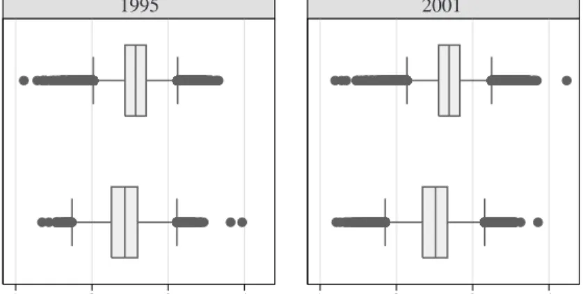
It clearly shows that workers with individual contracts get on average lower wages compared to their collectively covered colleagues whereas wage dispersion is somewhat higher. Further-more, the wage gap between the groups of covered and non-covered workers has increased over the observed years which is due to the observation that the average wage increase of workers with individually agreed contracts (about 3.3%) is lower than the wage increase of workers equipped with industry-level contracts (about 4.5%) and particularly than the ones with firm-level contracts (about 6.3%).14 _{Despite a slightly higher increase of total wages and wage}

dispersion of firm-level wages over time, wages of workers covered by industry-level contracts and firm-level contracts do hardly differ from each other what comes as no surprise since the wage-setting of firms using firm-level contracts usually conforms to unions’ collective bargain-ing agreements. Figure 1 clarifies the just mentioned findings in comparing the box-plots of all wage-setting regimes in 1995 and 2001. Here, the median is displayed by the line in the middle of the box, whereas the boundaries represent the respective 25th _{and 75}th _percentiles.

The longer the boxes and the more outliers - illustrated as circles - are present, the larger is the observed wage dispersion, respectively.

1995 2001

log gross hourly wage

1

1 2 3 4 2 3 4

individual collective

Figure 1: Boxplots of blue-collar workers’ log gross hourly wages in West Germany sorted by

wage-setting regime and by year.

Concerning the covariates, we focus on a comparison of characteristics between collectively covered workers and workers with individually agreed contracts since we find it reasonable on the basis of the just mentioned findings to band workers with industry-level contracts and workers with firm-level contracts together.

(16)

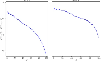
F − 1 co v ere d ( θ ) − F − 1 n o n -c o v ere d ( θ ) θ θ 1995 2001 20 20 40 60 80 100 0 40 60 80 100 0 0 -.2 .2 .4

Figure 2: Quantile differences between covered and non-covered blue-collar workers’ log gross

hourly wages in West Germany.

An additional look at the raw difference of the wage quantiles between covered and non-covered workers is presented in figure2. As already motivated the difference declines along the wage distribution. The difference is positive in the lower quantiles and gets even negative in 1995 from the third quartile on. In 2001 a negative difference can only be observed with the highest quantiles.

In table4descriptive statistics for all covariates except the industry dummies are reported. Con-cerning the human capital variables age, tenure and years of schooling, it becomes obvious that the only eye-catching difference between both groups of workers is given by average tenure, where covered workers’ tenure is on average 3.5 - 4 years higher than the one of non-covered workers. This applies to both years 1995 and 2001. Beyond the human capital variables a remarkable difference between both groups of workers can be detected concerning the female workforce: In 1995 about 16% of all covered workers were female compared to 25% of all non-covered workers. In 2001 this share has diminished in both groups which is attributable to a lower female labour participation in the manufacturing sector. We also find that workers with individually agreed contracts are on average less skilled than their collectively covered colleagues. While in both years more than half of the former are unskilled or semi-skilled, this share among covered workers amounts to about 45% in 1995 and 40% in 2001, respectively. Accordingly, high-skilled workers are more likely to be encountered among collectively covered workers. Concerning payment rules, the distinct majority of both groups gets paid according to a time wage in both years. While there are very little exceptions among noncovered workers

(17)

-especially in 2001 - virtually one of four covered workers is rewarded by an alternative payment rule like a bonus wage. The theoretical considerations concerning the connection between firm size and collective coverage of firms are confirmed by our empirical findings: While roughly three out of four non-covered workers are mainly employed in firms up to 199 employees in 2001, this share among covered workers amounts to merely 35.5% in the same year. Further it becomes obvious that the share of non-covered workers in firms with more than 1,000 employ-ees is relatively small (1995: 11%; 2001: 7%), whereas almost one third of all covered workers are employed in a large firm. Finally, concerning the age structure among the two groups it seems as younger workers tend to be rather equipped with individual contracts whereas aged employees are more likely to be paid according to a collective contract.

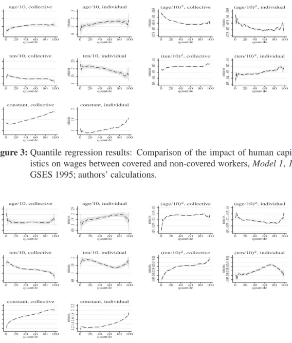
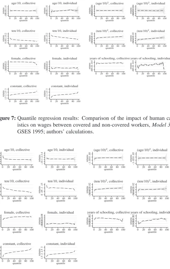
Above findings are well suited to describe the average differences between both groups’ char-acteristics and thus to provide some hints for the explanation of the total covered- non-covered wage gap. However, to identify the impact of groups’ characteristics on wages at various points of the wage distribution quantile regression coefficients need to be estimated. Estimation results for all explanatory variables are reported separately for each group, for each of the previously in-troduced models and sorted by years in tables (5)-(16). Exemplary, the human capital variables, the returns to female workers - available only for model 2 and 3 - and the constant representing a kind of base wage are additionally pictured in an analogous order in figures (3)-(8). Among the human capital variables it becomes obvious that tenure has by far the strongest impact on wages in both groups. However, in accordance with related literature like inFitzenberger et al.

(2007) tenure tends to be of particularly high importance for non-covered workers: we find in all three models unambiguously evidence that returns to tenure are highest for non-covered low-wage workers and lowest for covered high-wage workers, i.e. that a long tenure is most ad-vantageous for low-wage workers with individually agreed contracts and of inferior importance for covered high-wage workers, respectively. In contrast, but not surprisingly, we find much lower returns to female non-covered workers compared to their covered counterparts. Model 2 shows particularly for non-covered low-wage female workers in 2001 a highly negative impact on wages whereas covered high-wage female workers (model 3, 2001) suffer least from wage discrimination. In comparing both groups’ base wages, all three models make clear that base wages of covered standard workers are definitively higher than the ones of uncovered workers. Model 3, e.g., reports for 2001 log base wages of 2.0 in the bottom part and 2.6 in the top part of covered wage distributions. Uncovered base wages range merely from 1.9 to 2.2.

We now turn to the analysis of the components of between-groups’ wage differentials. Table2

(18)

Table 2: Blinder-Oaxaca-Decomposition of workers’ log gross hourly wages in West Germany,

1995 and 2001

1995 2001

Model 1 Model 2 Model 3 Model 1 Model 2 Model 3

total log wage difference 0.143 0.143 0.143 0.182 0.182 0.182

explained by characteristics 0.030 0.059 0.098 0.035 0.066 0.107 (0.000)*** (0.000)*** (0.000)*** (0.000)*** (0.000)*** (0.000)*** explained by bargaining 0.113 0.084 0.045 0.147 0.116 0.075

(0.000)*** (0.000)*** (0.000)*** (0.000)*** (0.000)*** (0.000)*** number of observations 282,037 282,037 282,037 179,711 179,711 179,711

p values based on bootstrapped standard errors (500 replications) in parentheses;

* significant at 10% ** significant at 5%; *** significant at 1%; Source: GSES 1995/2001, authors’ calculations.

wages according to the Blinder-Oaxaca-Decomposition given by equation (1). It becomes ob-vious that the total log wage spread between covered and non-covered workers has on average widened over the observed years from 0.143 (conforms to 1.15e_{) in 1995 to 0.182 (conforms}

to 1.20e_{) in 2001. Model 1 using only human capital variables, explains these wage}

differen-tials mainly by the bargaining effect which reflects in our study the amount of the wage gap that is due to the coverage by a collective contract. In both years it accounts for about four fifth of the total wage gap. However, the relative importance of the characteristics effect specifying the justified wage differential rises if further explaining variables are considered like in model 2. In-cluding all available explaining variables, the characteristics effect even exceeds the bargaining effect (model 3), i.e. that the average log wage advantage of covered workers of 0.182 in 2001 compared to their non-covered counterparts is particularly due to their characteristics and only to a minor part to coverage (characteristics: 0.107; bargaining: 0.075). Furthermore, it becomes obvious that the increase of the total wage gap in 2001 is mostly explained by the bargaining effect and is consequently only to a minor part attributable to the characteristics effect.

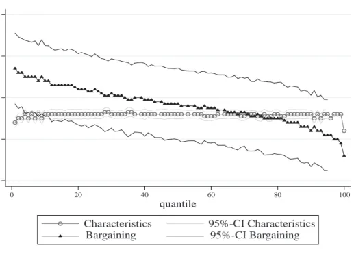
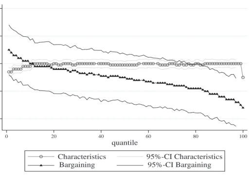
However, if not only mean effects are considered in order to explain the covered- non-covered wage differential, we detect substantial differences within groups’ wage distributions as can be seen in figures (9)-(14) where all results are based on Melly’s decomposition technique for quantile regressions. All three models show unambiguously for both years that the bargaining effect is highest in the lower parts of groups’ wage distributions whereas it decreases steadily with increasing wages. In 1995, it appears that the bargaining effect runs out of significance15

in the upper quantiles in model 1. Since the level of the bargaining effect decreases with more variables included, it becomes insignificant in the upper half of the wage distribution in model 2 and is almost completely insignificant in model 3. A comparison with the models 1-3 in 2001

(19)

clearly indicates a strengthening of the bargaining effect as its total level rises in all parts of the respective wage distributions.

Unlike the bargaining effect the characteristics effect is in all three models of both years highly significant and positive at any point of the wage distributions. Good characteristics pay off most for high-wage workers even though the characteristics effect increases only slightly across the wage distributions. Since the main portion of the total wage gap increase in 2001 is attributable to the bargaining effect, it comes as no surprise that the characteristics effect has virtually not changed over time.

Summing up, it can be ascertained that the total wage gap between covered and non-covered workers is for low-wage workers particularly due to collective coverage whereas individual characteristics are of minor importance. In contrast, the relative importance of individual char-acteristics rises with increasing workers’ remuneration so that the wage advantage of covered high-wage workers compared to their non-covered colleagues results mostly from better char-acteristics and is only to a minor part attributable to the coverage status. However, since the widening of the wage gap over time is mostly explained by the bargaining effect, the relative importance of coverage gains weight over time.

5 Conclusions and Outlook

This paper investigates the covered- non-covered wage gap in Germany. Descriptive Evidence using the GSES reports a gap of approximately 1.15 e_{in 1995 which increases to 1.20} e_in

2001. Theoretical considerations point out that this gap might result from union bargaining as well as from a non-random selection of workers into covered and non-covered firms, respec-tively. Using theMelly (2006) estimator which follows the Machado/Mata(2005) decompo-sition technique, it could be shown that the covered- non-covered wage gap results from two parts. The union bargaining effect is highest for workers in the lowest quantiles and decreases steadily in higher quantiles. This confirms the hypotheses that unions aim to compress the wage distribution especially for low-skilled workers. The highly significant characteristics effect can be interpreted as a result from the underlying selection of higher skilled workers in covered firms. In finding higher base wages and reduced returns to human capital for covered work-ers as unions narrow inequality across skill groups our results are in accordance to the related studies for Germany (cf.Fitzenberger et al. 2007,Stephan/Gerlach 2005).

(20)

Since the GSES does not only provide information about blue-collar workers in West Ger-many, the objective of prospective analysis could focus on the examination of the covered-non-covered wage gap of white-collar workers including employees in East Germany. Further, this study considers only collective and individual bargaining agreements. Unfortunately the GSES has no panel dimension to control for unobservable heterogeneity. However, more flexi-ble wage-setting regimes increasingly become important that should also be taken into account in future analysis.

(21)

References

Albrecht, J./A. Björklund/S. Vroman (2003): Is There a Glass Ceiling in Sweden?, in: Journal

of Labor Economics, 21(1), p. 145–177.

Albrecht, J. W./A. van Vuuren/S. Vroman (2004): Decomposing the Gender Wage Gap in the Netherlands with Sample Selection Adjustments, Discussion Paper 1400, IZA, Bonn. Blanchflower, D. G./A. Bryson (2004): What Effect Do Unions Have on Wages Now and Would

Freeman and Medoff Be Surprised?, in: Journal of Labor Research, 25(3), p. 383–414. Blinder, A. S. (1973): Wage Discrimination: Reduced Form and Structural Estimates, in: The

Journal of Human Resources, 8(4), p. 436–455.

Büttner, T./B. Fitzenberger (1998): Central Wage Bargaining and Local Wage Flexibility: Evi-dence from the Entire Wage Distribution, Discussion Paper 98-32, ZEW, Mannheim.

Card, D. (1996): The Effect of Unions on the Structure of Wages: A Longitudinal Analysis, in:

Econometrica, 64(4), p. 957–979.

Card, D./T. Lemieux/W. C. Riddell (2004): Unions and Wage Inequality, in: Journal of Labor

Research, 25(4), p. 519–562.

Dustmann, C./U. Schönberg (2004): Training and Union Wages, Discussion Paper 1435, IZA, Bonn.

Fitzenberger, B./K. Kohn/A. Lembcke (2007): Union Wage Effects in Germany: Union Density or Collective Bargaining Coverage?, Discussion Paper , Universität Frankfurt.

Frank-Bosch, B. (2003): Verdienststrukturen in Deutschland, in: Wirtschaft und Statistik, 2003(12), p. 1137–1151.

Freeman, R. B. (1982): Union wage practices and wage dispersion within establishments, in:

Industrial and Labor Relations Review, 36, p. 3–21.

Freeman, R. B./J. L. Medoff (1984): What do unions do?, Basic Books, New York.

Groshen, E. L. (1991): Five Reasons Why Wages Vary among Employers, in: Industrial

Rela-tions Journal, 30(3), p. 350–381.

Gürtzgen, N. (2006): The Effect of Firm- and Industry-Level Contracts on Wages - Evi-dence from Longitudinal Linked Employer-Employee Data, Discussion Paper 06-082, ZEW, Mannheim.

(22)

Hafner, H.-P. (2006): Gehalts- und Lohnstrukturerhebung im Produzierenden Gewerbe und im Dienstleistungsbereich 2001, in: Forschungsdatenzentrum der Statistischen Landesämter, Editor, Amtliche Mikrodaten für die Sozial- und Wirtschaftswissenschaften, Beiträge zu den

Nutzerkonferenzen des FDZ der Statistischen Landesämter 2005, p. 179–189.

Hall, P./S. J. Sheather (1988): On the Distribution of a Studentized Quantile, in: Journal of the

Royal Statistical Society, Series B, 50, p. 381–391.

Heinbach, W. D. (2007): Wages in Wage-Setting Regimes with Opening Clauses, in: AStA –

Wirtschafts- und Sozialstatistisches Archiv, 1(3), p. 233–245.

Hendricks, W./R. Koenker (1992): Hierarchical Spline Models for Conditional Quantiles and the Demand for Electricity, in: Journal of the American Statistical Association, 87(417), p. 58–68.

Hirsch, B. T. (2004): What Do Unions Do for Economic Performance?, in: Journal of Labor

Research, 25(3), p. 415–455.

Koenker, R./G. Bassett (1978): Regression Quantiles, in: Econometrica, 46(1), p. 33–50. Kohn, K. (2006): Rising Wage Dispersion, After All! The German Wage Structure at the Turn

of the Century, Discussion Paper 2098, IZA, Bonn.

Lewis, H. G. (1986): Union Relative Wage Effects: a Survey, University of Chicago Press, Chicago.

Machado, J./J. Mata (2005): Counterfactual Decomposition of Changes in Wage Distributions Using Quantile Regression, in: Journal of Applied Econometrics, 20(19), p. 445–465. Melly, B. (2006): Estimation of Counterfactual Distributions Using Quantile Regression,

Dis-cussion paper, SIAW, University of St. Gallen.

Mincer, J. (1974): Schooling, experience, and earnings, Human behavior and social institutions, National Bureau of Economic Research, New York.

Oaxaca, R. (1973): Male-Female Wage Differentials in Urban Labor Markets, in: International

Economic Review, 14(3), p. 693–709.

Sanner, H. (2006): Imperfect Goods and Labor Markets, and the Union Wage Gap, in: Journal

of Population Economics, 19(1), p. 119–136.

Stephan, G./K. Gerlach (2005): Wage settlements and wage setting: results from a multi-level model, in: Applied Economics, 37(20), p. 2297–2306.

(23)

A Decomposition of Wage Differences Across Wage Distributions

Blinder-Oaxaca-Decomposition

To quantify the components of a wage gap between two groups Blinder (1973) and Oaxaca

(1973) first developed a decomposition technique that detects the sources of the difference in the means. This approach proved to be particularly useful in explaining the differences in average log wagesY¯tbetween two groups t = (0; 1), i.e. between a favoured or treated group

indexed witht= 1and a discriminated or non-treated group indexed witht = 0. By assuming that the expected value ofY conditionally onXis a linear function ofX,

E[Yt|T = t]can be estimated consistently via OLS byX¯tβˆt, where the groups’ average

char-acteristicsX¯tcan be obtained by

1

nt

X

i:T=t

Xi and the corresponding coefficientsβˆtare resulting

from the regressions ofYtonXt. Then, sinceY¯t = ¯Xtβˆt, the difference betweenY¯1andY¯0can

be written as

¯

Y1−Y¯0 = ¯X1βˆ1−X¯0βˆ0. (3)

Addition and simultaneous subtraction of the counterfactualX¯0βˆ1 gives

¯

Y1−Y¯0 = ¯X1βˆ1(−X¯0βˆ1+ ¯X0βˆ1)−X¯0βˆ0. (4)

Then, the Blinder-Oaxaca-Decomposition is given by

¯ Y1−Y¯0 = ( ¯X1βˆ1−X¯0βˆ1) | {z } characteristics + ( ¯X0βˆ1−X¯0βˆ0) | {z } coefficients . (5)

Alternatively, the difference betweenY¯0 andY¯1 can be decomposed in an analogous way as

¯ Y0−Y¯1 = ( ¯X0βˆ0−X¯1βˆ0) | {z } characteristics + ( ¯X1βˆ0−X¯1βˆ1) | {z } coefficients . (6)

By introducing the counterfactualsX¯0βˆ1 as well as X¯1βˆ0, Blinder(1973) andOaxaca (1973)

(24)

determines the magnitude of the resulting wages. In the literature these two effects are com-monly known as characteristics effect - given by the first bracket in equations (5) and (6) -and as coefficients effect - the term in the second bracket in (5) and (6). The characteristics effect reflects the justified wage differential between both groups due to different productivities depending on the groups’ characteristics whereas the rest of the observable wage gap is con-tributable to the coefficients effect which honors the simple belonging to the treated group or punishes the simple belonging to the non-treated group. This becomes clear if e.g. equation (5) is rewritten as ¯ Y1−Y¯0 = ( ¯X1−X¯0) ˆβ1 | {z } characteristics + ( ˆβ1−βˆ0) ¯X0 | {z } coefficients . (7) Machado-Mata-Decomposition

Machado/Mata(2005) present an estimator using quantile regression to decompose differences in log wages between two groups since this overcomes the large waste of information if not only means of variables are considered but also differences at various quantiles of distributions can be analysed. Another important feature of quantile regression is its robustness against outliers. Assuming linearity between the quantiles of the dependent variable Y and the covariates X, then theτth conditional quantile ofY is given by

QY(τ|X) = Xβ(τ), ∀τ ∈(0,1). (8)

Koenker/Bassett(1978) solve by minimizing inβ(τ) ˆ β(τ) = min β∈R Kn −1 " _n X i ρτ(Yi−Xiβ) # , (i= 1, ..., n), (9)

where the check functionρτ weights asymmetrically the residualsui so that

ρτ(ui) =

(

τ ui for ui ≥0

(τ−1)ui for ui <0

(10)

Following Machado/Mata (2005) who propose an estimator of counterfactual unconditional wage distributions based on quantile regressions, the difference of theθthunconditional quantile

(25)

between two groups’ distributions can be decomposed according toBlinderandOaxaca(1973) as ˆ F−1 Y1 (θ|T = 1)− ˆ F−1 Y0 (θ|T = 0) = ˆ F−1 Y1 (θ|T = 1)− ˆ F−1 Y1 (θ|T = 0) | {z } characteristics (11) + Fˆ−1 Y1 (θ|T = 0)−Fˆ −1 Y0 (θ|T = 0) | {z } coefficients , or inversely as ˆ F−1 Y0 (θ|T = 0)− ˆ F−1 Y1 (θ|T = 1) = ˆ F−1 Y0 (θ|T = 0)− ˆ F−1 Y0 (θ|T = 1) | {z } characteristics (12) + Fˆ−1 Y0 (θ|T = 1)−Fˆ −1 Y1 (θ|T = 1) | {z } coefficients , whereFˆ−1 Yt (θ|T = t)denotes theθ

th _{unconditional quantile of group}_t_{’s wage. Again, the}

un-conditional counterfactual quantiles Fˆ−1

Y1 (θ|T = 0)as well as

ˆ

F−1

Y0 (θ|T = 1) in the terms on

the right hand side of (11) and (12) are needed to detect the mentioned effects at any uncondi-tional quantile. Even though an appropriate method of consistently estimating the variance is not presented in Machado’s and Mata’s (2005) pioneer work, several authors make use of this decomposition technique in their applications (cf. e.g.Albrecht et al. 2003,2004,Kohn 2006). But more importantly,Melly(2006) shows that their estimator only yields good MSE-properties if the number of quantile regression coefficientsm is large or goes at best to infinity since its variance vanishes.16 _{So if a data set is relatively small, one can increase}_m_{without losing too}

much computation time. However, many applications like ours are based on large or even huge data sets for which choosing the rightm is a sensitive question since estimation time depends crucially onmandn. The situation even worsens if the standard errors need to be bootstrapped in order to obtain reliable inference statistics. In our application we forgo bootstrapping since computation is simply infeasible. We computed analytic standard errors using the Hendricks-Koenker-sandwich estimator (Hendricks/Koenker 1992) employing Hall/Sheather (1988) rule for optimal bandwith.

16_If_m_{→ ∞}_{, the MSE of Machado’s and Mata’s estimator (}_{M SE}

MM) reduces to the bias that does not depend on

(26)

Melly-Estimator for Unconditional Counterfactual Distributions

For this reasonMelly (2006) presents an alternative estimator of counterfactual unconditional distributions that copes with this challenge. On the one hand he shows that Machado’s and Mata’s estimator is numerically equivalent to his own estimator if m goes to infinity. On the other hand - and most importantly for applications using large data sets - he proves that the MSE of his estimator (M SEMelly) does, in contrast to M SEMM, not depend on m and thus

M SEMelly ≤ M SEMM.17 In a nutshell, decomposition analysis based on quantile regression technique using large data sets become feasible. Since Melly’s estimator of counterfactual un-conditional distributions is relatively new and the basis of our application, the formal proceeding is briefly presented in the following.

After having estimated all conditional quantiles of Y given X by linear quantile regression,

Melly(2006) executes several calculation steps in order to obtain the unconditional quantiles of interest: For this purpose, he first estimates the conditional distribution ofYtgivenXiatq18by

ˆ FYt(q|Xi) = Z 1 0 1(Xiβˆt(τ)≤q)dτ = J X j=1 (τj−τj−1)1(Xiβˆt(τj)≤q), (13)

since is not possible to simply integrate the conditional quantile function for lack of monotonic-ity. The magnitude of the expression (τj −τj−1) in equation (13) diminishes by nature with

growingm. Asmequals100in our application, we assume(τj−τj−1)to take a constant value

of0.01.

Having once estimated the conditional distribution of Yt, the unconditional distribution

func-tions can easily be computed in a second step by

ˆ FYt(q|T =t) = 1 nt X i:_Ti=t ˆ FYt(q|Xi). (14)

17_{A comparison of the Mean Squared Errors} _{(M SE)}_{of both estimators displayed as Relative}_{M SE} M SE_MM M SE_Melly

shows that form = n= 400theM SEMMis more than twice as large as theM SEMellyand respectively for

m= 1000still1.5-times as large (cf.Melly 2006, p. 41).

(27)

Then, the unconditional quantiles qˆt(θ) as well as the unconditional counterfactual quantiles

ˆ

qc1(θ)- based onX0βˆ1(τ)- andqˆc0(θ)- based onX1βˆ0(τ)- are given by equations (15), (16)

and (17), respectively: ˆ qt(θ) = inf{q: 1 nt X i:Ti=t ˆ FYt(q|Xi)≥θ} (15) ˆ qc1(θ) = inf{q : 1 n0 X i:Ti=0 ˆ FY1(q|Xi)≥θ} (16) ˆ qc0(θ) = inf{q : 1 n1 X i:_Ti=1 ˆ FY0(q|Xi)≥θ} (17)

Finally, the difference between the θth _{unconditional quantiles of both groups can be}

decom-posed in analogy toBlinder(1973) andOaxaca(1973) as

ˆ q1(θ)−qˆ0(θ) = (ˆq1(θ)−qˆc1(θ)) | {z } characteristics + (ˆqc1(θ)−qˆ0(θ)) | {z } coefficients , (18) or alternatively as ˆ q0(θ)−qˆ1(θ) = (ˆq0(θ)−qˆ_c0(θ)) | {z } characteristics + (ˆqc0(θ)−qˆ1(θ)) | {z } coefficients . (19)

(28)

B Tables

Table 3: Description of variables

Variable label Variable description age/10 worker’s age/10 in years (age/10)2

worker’s age/10 squared tenure/10 worker’s tenure/10 in years (tenure/10)2

worker’s tenure/10 squared years of schooling worker’s years of schooling

Dummies

female female worker

married married worker

unskilled worker labourer without special skills

semi-skilled worker worker without special skills but more than three months of tenure skilled workers worker with vocational education or longtime tenure

high-skilled worker worker with excellent skills and longtime tenure time wage worker is exclusively paid according to working time bonus wage worker is paid according to working time and bonus premia,

e.g. for product quantity or quality, respectively

piece wage worker is paid according to product quantity within a predetermined period bonus- and piece wage worker is paid according to a mixture of bonus- and piece wage

mixed wage worker is paid according to a mixture of time wage and bonus wage or piece wage firm size with 100-199 employees share of firms with 100-199 employees

firm size with 200-499 employees share of firms with 200-499 employees firm size with 500-999 employees share of firms with 500-999 employees firm size with 1000 or more employees share of firms with 1000 or more employees share of female share of female workers at firm-level share of unskilled share of unskilled workers at firm-level share of semi-skilled share of semi-skilled workers at firm-level share of skilled share of skilled workers at firm-level share of high-skilled share of high-skilled workers at firm-level share of workers younger than 25 years share of workers < 25 years at firm-level

share of workers between 25 and 30 years share of workers between 25 and 30 years at firm-level share of workers between 30 and 35 years share of workers between 30 and 35 years at firm-level share of workers between 35 and 40 years share of workers between 35 and 40 years at firm-level share of workers between 40 and 45 years share of workers between 40 and 45 years at firm-level share of workers between 45 and 50 years share of workers between 45 and 50 years at firm-level share of workers with more than 50 years share of workers > 50 years at firm-level

firm in Hamburg or Schleswig-Holstein firm located in Hambourg or Schleswig-Holstein firm in Lower Saxony or Bremen firm located in Lower Saxony or Bremen firm in North Rhine-Westphalia firm located in North Rhine-Westphalia firm in Hesse firm located in Hesse

firm in Rhineland-Palatinate or Saarland firm located in Rhineland-Palatinate or Saarland firm in Bavaria firm located in Bavaria

(29)

Table 4: Deskriptive Statistics for covariates in 1995 and 2001

individual collective total

Variable year mean sd d9/d1 mean sd d9/d1 mean sd d9/d1

gross hourly wages 1995 11.73 3.09 1.95 13.40 2.95 1.72 13.24 3.00 1.76

2001 12.72 3.38 1.90 15.12 3.43 1.71 14.41 3.59 1.85

log gross hourly wages 1995 2.43 0.26 1.32 2.57 0.22 1.24 2.56 0.22 1.25

2001 2.51 0.26 1.29 2.69 0.22 1.22 2.64 0.25 1.26 age/10 1995 3.81 1.07 2.18 3.93 1.07 2.12 3.92 1.07 2.12 2001 3.95 1.04 2.09 4.05 1.00 2.01 4.02 1.02 2.04 tenure/10 1995 0.87 0.84 37.00 1.21 0.95 18.29 1.18 0.94 19.13 2001 0.81 0.82 34.71 1.23 0.97 23.21 1.10 0.95 27.55 years of schooling 1995 10.38 0.85 1.16 10.46 0.81 1.16 10.45 0.82 1.16 2001 10.39 0.94 1.22 10.52 0.84 1.16 10.49 0.87 1.16 female 1995 0.248 0.432 0.163 0.369 0.171 0.376 2001 0.167 0.373 0.117 0.321 0.131 0.338 unskilled worker 1995 0.228 0.420 0.178 0.382 0.183 0.387 2001 0.217 0.412 0.140 0.347 0.163 0.369 semi-skilled worker 1995 0.334 0.472 0.275 0.447 0.281 0.449 2001 0.322 0.467 0.257 0.437 0.276 0.447 skilled worker 1995 0.335 0.472 0.344 0.475 0.343 0.475 2001 0.370 0.483 0.359 0.480 0.362 0.481 high-skilled worker 1995 0.103 0.304 0.203 0.402 0.193 0.395 2001 0.091 0.288 0.244 0.430 0.199 0.399

firm size with 100-199 employees 1995 0.377 0.485 0.158 0.365 0.179 0.384

2001 0.768 0.422 0.355 0.479 0.476 0.499

2001 0.125 0.330 0.198 0.398 0.176 0.381

2001 0.035 0.183 0.131 0.337 0.103 0.304

firm size with 1000 or 1995 0.108 0.310 0.312 0.463 0.292 0.455

more employees 2001 0.073 0.260 0.316 0.465 0.245 0.430 share of. . . . . .female workers 1995 0.283 0.224 0.203 0.187 0.211 0.193 2001 0.210 0.212 0.161 0.166 0.175 0.182 . . .unskilled workers 1995 0.173 0.199 0.138 0.174 0.141 0.177 2001 0.166 0.212 0.116 0.164 0.131 0.181 . . .semi-skilled workers 1995 0.253 0.204 0.216 0.172 0.220 0.175 2001 0.253 0.217 0.204 0.188 0.218 0.198 . . .skilled workers 1995 0.257 0.195 0.272 0.193 0.271 0.193 2001 0.289 0.235 0.282 0.217 0.284 0.223 . . .high-skilled workers 1995 0.085 0.153 0.151 0.160 0.145 0.161 2001 0.086 0.148 0.181 0.193 0.153 0.186

. . .workers younger than 25 years 1995 0.104 0.072 0.075 0.051 0.078 0.054

2001 0.085 0.080 0.064 0.057 0.070 0.065

. . .workers between 25 and 30 years 1995 0.177 0.074 0.156 0.063 0.158 0.064

2001 0.117 0.083 0.100 0.064 0.105 0.071

2001 0.162 0.087 0.154 0.070 0.156 0.076

2001 0.177 0.088 0.184 0.071 0.182 0.076

2001 0.155 0.084 0.163 0.069 0.161 0.074

2001 0.125 0.078 0.135 0.067 0.132 0.070

. . .workers with more than 50 years 1995 0.170 0.097 0.203 0.096 0.200 0.097

2001 0.178 0.117 0.201 0.104 0.194 0.109

observations 1995 27,314 254,723 282,037

(30)

Table 5:Quantile regression coefficients for covered workers, Model 1, 1995

log gross hourly wages Q(10) Q(25) Q(50) Q(75) Q(90)

age/10 0.0765 0.0950 0.1196 0.1242 0.1192 (0.0060) (0.0037) (0.0035) (0.0037) (0.0053) (age/10)2 -0.0111 -0.0131 -0.0158 -0.0164 -0.0151 (0.0001) (0.0001) (0.0001) (0.0001) (0.0001) tenure/10 0.1497 0.1393 0.1330 0.1324 0.1285 (0.0026) (0.0016) (0.0015) (0.0016) (0.0024) (tenure/10)2 -0.0230 -0.0212 -0.0202 -0.0201 -0.0190 (0.0002) (0.0001) (0.0001) (0.0001) (0.0003) years of schooling 0.0809 0.0801 0.0735 0.0693 0.0676 (0.0012) (0.0006) (0.0005) (0.0006) (0.0008)

firm in Hamburg or Schleswig-Holstein -0.0217 -0.0205 -0.0192 -0.0189 -0.0045

(0.0036) (0.0022) (0.0023) (0.0028) (0.0040)

firm in Lower Saxony or Bremen -0.0649 -0.0648 -0.0748 -0.0851 -0.0888

(0.0025) (0.0019) (0.0016) (0.0019) (0.0022)

firm in North Rhine-Westphalia -0.0372 -0.0365 -0.0396 -0.0441 -0.0357

(0.0019) (0.0012) (0.0012 ) (0.0013) (0.0018)

firm in Hesse -0.0351 -0.0424 -0.0537 -0.0655 -0.0701

(0.0023) (0.0016) (0.0017) (0.0016) (0.0025)

firm in Rhineland-Palatinate or Saarland -0.0524 -0.0502 -0.0518 -0.0503 -0.0501

(0.0032) (0.0020) (0.0017) (0.0018) (0.0026)

firm in Bavaria -0.0925 -0.0828 -0.0862 -0.0954 -0.1027

(0.0019) (0.0011) (0.0010) (0.0012) (0.0017)

firm in Baden-Württemberg (reference)

Constant 1.2860 1.3801 1.5283 1.6928 1.8298

(0.0007) (0.0005) (0.0005) (0.0005) (0.0007)

Observations 254,723 254,723 254,723 254,723 254,723

Pseudo R2 0.111 0.113 0.107 0.099 0.092

analytic standard errors in parentheses, Source: GSES 1995; authors’ calculations

Table 6:Quantile regression coefficients for non-covered workers, Model 1, 1995

firm in Hamburg or Schleswig-Holstein -0.0085 0.0212 0.0323 0.0220 0.0194

(0.0103) (0.0077) (0.0058) (0.0085) (0.0082)

(0.0042) (0.0053) (0.0059) (0.0055) (0.0065)

(0.0045) (0.0051) (0.0050) (0.0048) (0.0066)

firm in Hesse -0.0219 -0.0096 -0.0199 -0.0185 -0.0322

(0.0044) (0.0047) (0.0041) (0.0057) (0.0075)

firm in Rhineland-Palatinate or Saarland -0.0168 0.0057 0.0128 0.0500 0.0435

(0.0051) (0.0065) (0.0043) (0.0065) (0.0047)

firm in Bavaria -0.1057 -0.0963 -0.0967 -0.1031 -0.1053

(0.0028) (0.0039) (0.0048) (0.0044) (0.0061)

Constant 0.9166 0.9172 1.0404 1.1283 1.2963

(0.0013) (0.0015) (0.0015) (0.0015) (0.0020)

Observations 27,314 27,314 27,314 27,314 27,314

Pseudo R2 0.157 0.164 0.16 0.146 0.13

(31)

firm in Hamburg or Schleswig-Holstein -0.0407 -0.0347 -0.0382 -0.0217 0.0253

(0.0048) (0.0034) (0.0032) (0.0039) (0.0066)

(0.0033) (0.0023) (0.0020) (0.0023) (0.0034)

(0.0028) (0.0019) (0.0017) (0.0021) (0.0029)

firm in Hesse -0.0157 -0.0248 -0.0395 -0.0675 -0.0719

(0.0032) (0.0028) (0.0021) (0.0023) (0.0032)

(0.0031) (0.0025) (0.0019) (0.0021) (0.0031)

firm in Bavaria -0.0504 -0.0623 -0.0664 -0.0710 -0.0675

(0.0024) (0.0017) (0.0017) (0.0023) (0.0027)

Constant 1.5360 1.6707 1.7872 1.9389 2.0219

(0.0010) (0.0007) (0.0006) (0.0007) (0.0010)

Observations 126,941 126,941 126,941 126,941 126,941

Pseudo R2 0.092 0.088 0.082 0.071 0.061

analytic standard errors in parentheses, Source: GSES 1995; authors’ calculations

firm in Hamburg or Schleswig-Holstein -0.0314 -0.0094 0.0258 0.0702 0.0929

(0.0058) (0.0047) (0.0044) (0.0058) (0.0075)

(0.0050) (0.0040) (0.0032) (0.0043) (0.0055)

(0.0035) (0.0035) (0.0025) (0.0035) (0.0054)

firm in Hesse -0.0195 -0.0056 -0.0020 0.0009 -0.0018

(0.0063) (0.0045) (0.0034) (0.0037) (0.0047)

(0.0057) (0.0035) (0.0036) (0.0040) (0.0066)

firm in Bavaria -0.0740 -0.0590 -0.0458 -0.0468 -0.0563

(0.0053) (0.0026) (0.0030) (0.0031) (0.0043)

Constant 1.2367 1.2536 1.3101 1.4646 1.6378

(0.0015) (0.0011) (0.0010) (0.0011) (0.0017)

Observations 52,770 52,770 52,770 52,770 52,770

Pseudo R2 0.102 0.12 0.119 0.11 0.108

(32)

age/10 0.0736 0.0742 0.0716 0.0640 0.0538 (0.0050) (0.0028) (0.0023) (0.0035) (0.0071) (age/10)2 -0.0092 -0.0094 -0.0095 -0.0087 -0.0071 (0.0043) (0.0031) (0.0029) (0.0034) (0.0049) tenure/10 0.0859 0.0792 0.0837 0.0872 0.0795 (0.0001) (0.0001) (0.0001) (0.0001) (0.0001) (tenure/10)2 -0.0162 -0.0144 -0.0148 -0.0149 -0.0125 (0.0017) (0.0012) (0.0013) (0.0015) (0.0022) years of schooling 0.0165 0.0149 0.0178 0.0207 0.0236 (0.0001) (0.0001) (0.0001) (0.0001) (0.0002) female -0.1947 -0.1752 -0.1540 -0.1583 -0.1579 (0.0007) (0.0005) (0.0005) (0.0006) (0.0008) married 0.0269 0.0238 0.0245 0.0241 0.0212 (0.0016) (0.0015) (0.0011) (0.0012) (0.0018)

unskilled worker (reference)

semi-skilled worker 0.0532 0.0567 0.0655 0.0679 0.0660 (0.0010) (0.0008) (0.0008) (0.0009) (0.0013) skilled worker 0.1325 0.1324 0.1358 0.1369 0.1424 (0.0016) (0.0013) (0.0012) (0.0013) (0.0017) high-skilled worker 0.2344 0.2283 0.2304 0.2367 0.2512 (0.0012) (0.0009) (0.0008) (0.0010) (0.0013)

time wage (preference)

bonus wage 0.0114 0.0201 0.0359 0.0394 0.0309

(0.0011) (0.0009) (0.0010) (0.0012) (0.0017)

piece wage 0.1069 0.1235 0.1243 0.1044 0.0793

(0.0016) (0.0013) (0.0013) (0.0014) (0.0019)

bonus- and piece wage 0.0757 0.0782 0.0808 0.0614 0.0384

(0.0016) (0.0012) (0.0010) (0.0010) (0.0014)

mixed wage 0.0124 0.0179 0.0172 0.0112 0.0068

(0.0083) (0.0060) (0.0055) (0.0046) (0.0066)

firm in Hamburg or Schleswig-Holstein -0.0480 -0.0445 -0.0432 -0.0442 -0.0282

(0.0030) (0.0019) (0.0016) (0.0022) (0.0028)

(0.0021) (0.0019) (0.0020) (0.0025) (0.0033)

(0.0019) (0.0013) (0.0012) (0.0015) (0.0022)

firm in Hesse -0.0543 -0.0627 -0.0749 -0.0779 -0.0753

(0.0013) (0.0010) (0.0010) (0.0011) (0.0016)

(0.0015) (0.0013) (0.0012) (0.0015) (0.0021)

firm in Bavaria -0.0868 -0.0883 -0.0959 -0.1012 -0.0952

(0.0021) (0.0014) (0.0013) (0.0018) (0.0020)

Constant 1.9393 2.0443 2.1144 2.2101 2.2979

(0.0011) (0.0009) (0.0009) (0.0010) (0.0014)

Observations 254,723 254,723 254,723 254,723 254,723

Pseudo R2 0.304 0.284 0.255 0.228 0.206

(33)

bonus wage 0.0804 0.0931 0.0987 0.0953 0.0860

(0.0074) (0.0049) (0.0027) (0.0028) (0.0082)

piece wage 0.0840 0.0899 0.0964 0.1022 0.0847

(0.0081) (0.0046) (0.0068) (0.0035) (0.0087)

(0.0019) (0.0061) (0.0058) (0.0056) (0.0074)

mixed wage 0.0454 0.0431 0.0428 0.0534 0.0708

(0.0125) (0.0169) (0.0075) (0.0036) (0.0140)

firm in Hamburg or Schleswig-Holstein -0.0113 0.0133 0.0309 0.0304 0.0470

(0.0076) (0.0038) (0.0072) (0.0047) (0.0075)

(0.0095) (0.0066) (0.0077) (0.0058) (0.0074)

(0.0044) (0.0034) (0.0040) (0.0045) (0.0074)

firm in Hesse -0.0519 -0.0555 -0.0660 -0.0621 -0.0542

(0.0035) (0.0033) (0.0032) (0.0032) (0.0056)

(0.0059) (0.0035) (0.0036) (0.0028) (0.0056)

firm in Bavaria -0.0845 -0.0862 -0.0918 -0.0911 -0.0706

(0.0011) (0.0043) (0.0021) (0.0013) (0.0052)

Constant 1.6128 1.7587 1.8510 1.9751 2.1032

(0.0049) (0.0020) (0.0039) (0.0029) (0.0044)

Observations 27,314 27,314 27,314 27,314 27,314

Pseudo R2 0.358 0.359 0.341 0.315 0.288

(34)

bonus wage 0.0267 0.0597 0.0885 0.0825 0.0622

(0.0018) (0.0013) (0.0012) (0.0016) (0.0024)

piece wage 0.0967 0.1249 0.1265 0.0990 0.0596

(0.0033) (0.0022) (0.0016) (0.0019) (0.0025)

(0.0047) (0.0031) (0.0020) (0.0021) (0.0028)

mixed wage 0.0464 0.0359 0.0337 0.0189 -0.0068

(0.0089) (0.0048) (0.0050) (0.0069) (0.0106)

firm in Hamburg or Schleswig-Holstein -0.0703 -0.0507 -0.0415 -0.0250 0.0153

(0.0033) (0.0019) (0.0021) (0.0030) (0.0037)

(0.0036) (0.0029) (0.0029) (0.0036) (0.0051)

(0.0028) (0.0017) (0.0017) (0.0021) (0.0034)

firm in Hesse -0.0281 -0.0356 -0.0542 -0.0679 -0.0605

(0.0021) (0.0015) (0.0014) (0.0018) (0.0025)

(0.0028) (0.0019) (0.0016) (0.0021) (0.0029)

firm in Bavaria -0.0619 -0.0663 -0.0744 -0.0757 -0.0598

(0.0027) (0.0020) (0.0016) (0.0020) (0.0029)

Constant 1.8955 2.0395 2.1573 2.2730 2.3469

(0.0019) (0.0016) (0.0014) (0.0017) (0.0025)

Observations 126,941 126,941 126,941 126,941 126,941

Pseudo R2 0.231 0.213 0.199 0.174 0.148