Investment-Based Expected Stock Returns

Investment-Based Expected Stock Returns

Laura Xiaolei Liu∗

School of Business and Management Hong Kong University of Science

and Technology

Toni M. Whited† Wisconsin School of Business

University of Wisconsin Lu Zhang‡

Stephen M. Ross School of Business University of Michigan

and NBER December 2008§

Abstract

Theq-theory provides a simple empirical structure for understanding the cross section of stock returns. Under constant returns to scale stock returns equal levered investment returns, which are tied directly to firm characteristics. We use GMM to match moments of levered investment returns to those of observed stock returns. The model captures the average stock returns of port-folios formed on earnings surprises, book-to-market equity, and capital investment. Volatilities predicted from the model are largely comparable to volatilities observed in the data. However, the model falls short in matching expected returns and volatilities simultaneously.

∗_{Finance Department, School of Business and Management, Hong Kong University of Science and Technology,} Kowloon, Hong Kong. Tel: (852) 2358-7661, fax: (852) 2358-1749, and e-mail: [email protected].

†_{Wisconsin School of Business, University of Wisconsin, Madison, 975 University Avenue, Madison WI 53706.} Tel: (608) 262-6508, fax: (608) 265-4195, and e-mail: [email protected].

‡_{Finance Department, Stephen M. Ross School of Business, University of Michigan, 701 Tappan E 7605 Bus Ad,} Ann Arbor MI 48109-1234; and NBER. Tel: (734) 615-4854, fax: (734) 936-0282, and e-mail: [email protected]. §_{We have benefited from helpful comments of Nick Barberis, David Brown, V. V. Chari, Du Du, Simon Gilchrist,} Rick Green, Burton Hollifield, Liang Hu, Patrick Kehoe, Bob King, Narayana Kocherlakota, Leonid Kogan, Owen Lamont, Sydney Ludvigson, Ellen McGrattan, Antonio Mello, Jianjun Miao, Mark Ready, Bryan Routledge, Martin Schneider, Jun Tu, Masako Ueda, and other seminar participants at Boston University, Brigham Young University, Federal Reserve Bank of Minneapolis, Carnegie Mellon University, Emory University, Erasmus University Rotterdam, Florida State University, HKUST, INSEAD, London Business School, London School of Economics, New York University, Purdue University, Renmin University of China, Tilburg University, Yale School of Management, University of Arizona, University of Lausanne, University of Vienna, University of Wisconsin at Madison, Society of Economic Dynamics Annual Meetings in 2006, UBC PH&N Summer Finance Conference in 2006, American Finance Association Annual Meetings in 2007, and the 2007 China International Conference in Finance. Liu acknowledges financial support from HKUST (grant number SBI07/08.BM04). This paper supersedes our NBER working paper #11323 titled “Regularities.” All remaining errors are our own.

1

Introduction

We use the q-theory of investment to provide an empirical structure for studying the cross section of expected stock returns. The theory’s assumption of constant returns to scale implies that stock returns equal levered investment returns, which are directly tied to firm characteristics through optimality conditions. We use GMM to match the means and variances of levered investment re-turns with those of stock rere-turns. As testing assets we use portfolios motivated by well-documented patterns in cross-sectional returns: those formed on earnings surprises, book-to-market equity, and investment (e.g., Ball and Brown 1968, Fama and French 1993, and Titman, Wei, and Xie 2004).

The investment-based model outperforms traditional asset pricing models in matching expected returns. We estimate an average pricing error of 0.74% per annum for ten portfolios formed on earnings surprises. This error is much lower than those from the CAPM, 5.67%, the Fama-French (1993) model, 4.01%, and the standard consumption CAPM with CRRA utility, 3.62%. Further, the errors in the investment model do not vary systematically with earnings surprises: the error for the high-minus-low earnings portfolio is −0.40%, which is negligible compared to the errors from

the traditional models, which range from 12.55% to 14.06%. Although the investment model and the consumption CAPM produce almost identical average pricing errors across ten book-to-market portfolios (2.32% and 2.36%), the investment model produces an error for the high-minus-low port-folio of only 1.21%, which is substantially smaller than the error of 12.31% from the consumption CAPM. Finally, we estimate an average pricing error for ten investment portfolios of 1.51% per annum, which is smaller than the error of 2.35% from the consumption CAPM. More important, the high-minus-low investment portfolio has a much smaller error in the investment model than in the consumption CAPM: −0.49% versus −8.38%.

When we use the investment model to match both average returns and variances of the testing portfolios, variances predicted by the model are largely comparable to stock return variances, and their differences are insignificant. The average stock return volatility across the earnings surprise portfolios is 21.1% per annum, which is close to the average levered investment return volatility of 18.1%. The average realized and predicted volatilities are also close for the investment portfolios: 24.8% vs. 22.6%, and for the book-to-market portfolios: 25.0% vs. 18.6%. Across all testing port-folios, the average predicted volatility is about 16% lower than the average stock return volatility. However, the model falls short in two ways. First, while we find no discernible relation between vari-ances and firm characteristics in the data, the model predicts a positive relation between varivari-ances

and book-to-market. Second, average return errors vary systematically with earnings surprises and investment, and are comparable in magnitude to those from the traditional models. However, the investment model still does better in matching the average returns of the book-to-market portfolios. The intuition behind these results comes directly from the definition of the investment return from periodstto t+1, which is the marginal benefit of investment att+1 divided by the marginal cost of investment att. The definition suggests several economic forces driving the cross section of average stock returns. The first operates through the marginal benefit of investment, whose first component is the marginal product of capital at t+1 in the numerator of the investment return. The second component is roughly proportional to the growth rate of investment, which corresponds to the “capital gain” component of the investment return: investment is an increasing function of marginalq, which is related to the firm’s stock price. In the data firms with high earnings surprises have higher marginal products (measured by sales-to-capital) and investment growth than firms with low earnings surprises. These characteristics, combined with the equality of stock and levered investment returns, imply a positive relation between earnings surprises and expected stock returns. The third mechanism behind our results works through investment-to-capital at time t in the denominator of the investment return. Because investment today increases with the net present value of one additional unit of capital, and because the net present value decreases with the cost of capital, a low cost of capital means high net present value and high investment. Therefore, investment today and average returns are negatively correlated. Finally, because investment is also an increasing function of marginal q, and because marginal q is in turn inversely related to book-to-market equity, expected stock returns and book-to-market equity are positively correlated. Althoughq-theory originates in Brainard and Tobin (1968) and Tobin (1969), our work is built more directly on Cochrane (1991), who first usesq-theory to study the time series of aggregate stock returns, thereby launching the now active literature on investment-based asset pricing. Cochrane (1996) uses aggregate investment returns to parameterize the stochastic discount factor in cross-sectional tests. Several more recent articles model cross-cross-sectional returns based on firms’ dynamic optimization problems (e.g., Berk, Green, and Naik 1999, Carlson, Fisher, and Giammarino 2004, and Zhang 2005). Our work stands apart from these studies because we do structural estimation of closed-form Euler equations. Our work is also connected to the literature that estimates investment Euler equations using aggregate or firm level investment data (e.g., Shapiro 1986 and Whited 1992). Our work differs by restating the investment Euler equation in terms of returns and testing it with

both portfolio return and investment data. Finally, our evidence supports several recent articles showing that q-theory provides a surprisingly good description of investment behavior.1

2

The Model of the Firms

Time is discrete and the horizon infinite. Firms use capital and costlessly adjustable inputs to pro-duce a homogeneous output. These latter inputs are chosen each period to maximize operating prof-its, defined as revenues minus the expenditures on these inputs. Taking operating profits as given, firms choose optimal investment to maximize the market value of equity. Letπj_t≡π(kjt, x

j

t) denote the maximized operating profits of firmjat timet. The profit function depends on capital,kj_t, and a vector of exogenous aggregate and firm-specific shocks,xj_t, and it exhibits constant returns to scale.

End-of-period capital equals investment plus beginning-of-period capital net of depreciation:

kj_t+1 =ij_t+ (1−δjt)k

j

t, (1)

in which capital depreciates at an exogenous proportional rate of δj_t, which is firm-specific and time-varying. Firms incur adjustment costs when investing. The adjustment cost function, denoted

φ(ij_t, kj_t), is increasing and convex inij_t, decreasing in k_tj, and linearly homogeneous in ij_t andkj_t. Firms can finance investment with debt. For simplicity, we follow Hennessy and Whited (2007) and model only one-period debt. At the beginning of time t, firmj can issue an amount of debt, denoted bj_t+1, which must be repaid at the beginning of period t+ 1. The gross corporate bond return on bj_t, denoted ιj_t, can vary across firms and through time.

Taxable corporate profits equal operating profits less capital depreciation, adjustment costs, and interest expenses (e.g., Hall and Jorgenson 1967 and Hubbard, Kashyap, and Whited 1995):

Taxable corporate profits≡π(kjt, x j t)−δ j tk j t −φ(i j t, k j t)−(ι j t−1)b j t. (2)

Adjustment costs are expensed, consistent with treating them as forgone operating profits. Let τt denote the corporate tax rate at time t. We can write the payout of firmj as:

dj_t ≡(1−τt)[π(kjt, x j t)−φ(i j t, k j t)]−i j t +b j t+1−ι j tb j t+τtδjtk j t+τt(ι j t −1)b j t, (3)

1_{Erickson and Whited (2000) show that after controlling for measurement error in Tobin’sq, a simple regression} of investment on Tobin’sq has anR2 of almost 50%, and no other variables matter for investment. Eberly, Rebelo, and Vincent (2008) show that models based on Hayashi (1982) provide a good description of investment behavior at the firm level and that investment regressions are uninformative about the model’s performance. Philippon (2008) shows that a measure ofqfrom bond prices fits an investment regression well.

in which τtδjtk j

t is the depreciation tax shield andτt(ι j t−1)b

j

t is the interest tax shield.

Letmt+1be the stochastic discount factor fromttot+ 1, which is correlated with the aggregate

component ofxj_t+1. We can formulate the cum-dividend market value of equity as follows:

vj_t ≡ max {ij_t+s,k_tj_+s+1,bj_t+s+1}∞ s=0 Et " _∞ X s=0 mt+sdjt+s # , (4)

subject to the capital accumulation equation (1) and a transversality condition that prevents firms from borrowing an infinite amount to distribute to shareholders: limT→∞Et

h

mt+T bjt+T+1

i

= 0. Letq_tj be the present value multiplier associated with equation (1). The optimality conditions with respect to ij_t, kj_t+1, andbj_t+1 are, respectively,

qj_t = 1 + (1−τt) ∂φ(ij_t, kj_t) ∂ij_t (5) qj_t =Et " mt+1 " (1−τt+1) " ∂π(k_tj₊₁, xj_t+1) ∂kj_t+1 − ∂φ(ij_t+1, kj_t+1) ∂kj_t+1 # +τt+1δjt+1+ (1−δ j t+1)q j t+1 ## (6) 1 =Et h mt+1 h ιj_t+1−(ιjt+1−1)τt+1 ii . (7)

Equation (5) is the optimality condition for investment. It equates the marginal purchase and adjustment costs of investing to the marginal benefit,q_tj(marginalq), which is the expected present value of the marginal profits from investing in one additional unit of capital. Equation (6) is the investment Euler condition, which describes the evolution of qj_t. The term (1−τt+1)

∂π(kj_t+1,xj_t+1)

∂kj_t+1 captures the marginal after-tax profit generated by an additional unit of capital at t+ 1,and the term −(1−τt+1)

∂φ(ij_t+1,k_tj₊₁)

∂k_tj₊₁ captures the marginal after-tax reduction in adjustment costs. The termτt+1δjt+1 is the marginal depreciation tax shield, and the term (1−δ

j t+1)q

j

t+1 is the marginal

continuation value of an extra unit of capital, net of depreciation. Discounting these marginal profits of investment dated t+ 1 back totusing the stochastic discount factor yields q_tj.

Equation (7) says thatEt[mt+1ιjt+1] = 1+Et[mt+1(ιjt+1−1)τt+1]. Intuitively, because of the tax

benefit of debt, the unit price of the pre-tax bond return, Et[mt+1ιjt+1], is higher than unity. The

difference is precisely the present value of the tax benefit. If we define the after-tax bond return as:

rj_Bt+1 ≡ιjt+1−(ι

j

t+1−1)τt+1, (8)

Dividing both sides of equation (6) byqj_t and substituting equation (5), we obtain:

Et[mt+1rItj+1] = 1, (9)

in which r_Itj₊₁ is the investment return, defined as:

r_Itj₊₁ ≡ (1−τt+1) ∂π(k_tj₊₁,xj_t+1) ∂k_tj₊₁ − ∂φ(ij_t+1,kj_t+1) ∂k_tj₊₁ +τt+1δjt+1+ (1−δ j t+1) 1 + (1−τt+1) ∂φ(ij_t+1,k_tj₊₁) ∂ij_t+1 1 + (1−τt)∂φ(i j t,k j t) ∂ij_t . (10) The first order conditions (5) and (6) imply that the investment return is the ratio of the marginal benefit of investment at time t+ 1 divided by the marginal cost of investment att. The first term in brackets in the numerator divided by the denominator is analogous to a dividend yield. The second term in brackets in the numerator divided by the denominator is analogous to a capital gain because equation (5) implies that this ratio is the growth rate of q_tj.

We follow the empirical investment literature in specifying the marginal product of capital and the adjustment cost function. Love (2003) shows that if firms have a Cobb-Douglas production function with constant returns to scale, the marginal product of capital of firmj is given by:

∂π(k_tj, xj_t)

∂kj_t =κ

y_tj

k_tj, (11)

in which yj_t is sales, and κ > 0 is capital’s share. This parametrization assumes that shocks to operating profits,xj_t, are reflected in sales. We use a standard quadratic adjustment cost function:

φ(ij_t, k_tj) =a 2 ij_t kj_t !2 k_tj. (12)

Plugging equations (11) and (12) into the investment return equation (10), we obtain:

r_Itj₊₁ ≡ (1−τt+1) " κy j t+1 kj_t+1 + a 2 ij_t+1 kj_t+1 2# +τt+1δjt+1+ (1−δ j t+1) 1 + (1−τt+1)a ij_t+1 k_tj₊₁ 1 + (1−τt)a _ij t k_tj . (13) Definepj_t ≡vtj−d j

t as ex-dividend equity value,r j St+1 ≡(p j t+1+d j t+1)/p j

t as the stock return, and

νjt≡bjt+1/(p

j t +b

j

t+1) as market leverage. Appendix A shows that under constant returns to scale,

and that the investment return is the weighted average of the stock and after-tax bond returns:

r_Itj₊₁ =νj_tr_Btj ₊₁+ (1−νjt)r

j

St+1. (15)

Equation (15) is exactly the weighted average cost of capital in corporate finance (e.g., Berk and DeMarzo 2007, p. 465).2 _{Without leverage, equation (15) reduces to the equivalence between stock}

and investment returns, a relation first established by Cochrane (1991) and Restoy and Rockinger (1994). This relation is an algebraic restatement of the link between marginal q and average q as in Lucas and Prescott (1971), Hayashi (1982), and Abel and Eberly (1994).

3

Econometric Methodology

Section 3.1 presents the basic framework, and Section 3.2 details our empirical procedure.

3.1 Framework

Solving for r_Stj ₊₁ from equation (15) gives:

r_Stj ₊₁ =Lrj_It+1≡ rj_It+1−νjtr j Bt+1 1−νjt , (16)

in which Lrj_It+1 is the levered investment return, which is directly tied to firm characteristics.

3.1.1 GMM Estimation and Tests

To test whether cross-sectional variation in average stock returns corresponds to cross-sectional variation in firm characteristics, we test the ex-ante restriction implied by equation (16): expected stock returns equal expected levered investment returns,

Ehrj_St+1−LrjIt+1

i

= 0. (17)

A long-standing puzzle in financial economics is that stock returns are excessively volatile (e.g., Shiller 1981). Cochrane (1991) reports that the volatility of annual aggregate investment return is only about 60% of the volatility of annual value-weighted stock market returns. To study whether the investment-based model can reproduce empirically plausible stock return volatilities, we test

2_{Define ˜ι}j t+1≡ι

j

t+1−1 as the net pre-tax corporate bond return. The after-tax bond return from equation (8) is

rBtj +1= 1 + (1−τt+1)˜ιjt+1. Pluggingr

j

whether stock return variances equal levered investment return variances: E rj_St+1−E h rj_St+1i2− Lrj_It+1−E h Lr_Itj₊₁ i2 = 0. (18)

This equation is equivalent toσ2_rj St+1 −σ2 LrjIt+1 = 0, in whichσ2₍

·) denote the unconditional

variance of the series in the parentheses.

We estimate the parametersaandκusing GMM on equation (17) or on equations (17) and (18) jointly at the portfolio level. Using portfolios makes sense. First, empirical regularities in the cross section of returns can always be represented using the popular Fama and French (1993) portfolio approach. The portfolio approach also is widely used in the practice of quantitative investment management (e.g., Chincarini and Kim 2006). Second, investment Euler equations fit well at the portfolio level because portfolio investment data are relatively smooth. Thomas (2002) shows that aggregation substantially reduces the effect of lumpy investment in equilibrium business cycle models. Although simple Euler equations are rejected at the firm level because of lumpy investment, as in Whited (1998) and Abel and Eberly (2001), Hall (2004) shows that the effect of nonconvex adjustment costs is unimportant for estimating investment Euler equations at the industry level.

We use one-stage GMM with the identity weighting matrix to preserve the economic structure of the testing portfolios. After all, we choose testing portfolios precisely because the underlying characteristics are economically important in providing a wide spread in the cross section of average stock returns. The identity weighting matrix also gives potentially more robust, albeit less efficient, estimates. The estimates from second-stage or iterated GMM (not reported) are similar to the first-stage estimates. To conduct inferences, we nevertheless need to calculate the optimal weighting matrix. We use a standard Bartlett kernel with a window length of five. The results are insensitive to the window length. To test whether all (or a subset of) model errors are jointly zero, we use a

χ2 test from Hansen (1982, Lemma 4.1). Appendix B provides additional econometric details.

3.1.2 Discussion

As noted by Cochrane (1991), equation (16), taken literally, says that levered investment returns equal stock returns at every data point. This prediction is formally rejected at any level of sig-nificance. To construct an economically meaningful test, we must add distributional assumptions about the errors. In our implementation we assume that the model errors given by the empirical counterparts of the left-hand side of equations (17) and (18) both have a mean of zero. While

rec-ognizing that measurement errors and specification errors, unlike forecast errors, do not necessarily satisfy this assumption, we note that similar assumptions underlie most Euler equation tests.3

Our investment Euler equation approach to the cross section of average stock returns differs from consumption-based Euler equation tests (e.g., Hansen and Singleton 1982 and Lettau and Ludvigson 2001) in that we do not use information on preferences. Equation (17) ties expected stock returns directly to firm characteristics without parameterizing the stochastic discount factor,

mt+1. However, mt+1 is important because it indirectly affects expected returns. If mt+1=m is

constant, equation (9) implies that the expected returnEt[rj_It+1] = 1/m, which is uncorrelated with firm characteristics. If operating profits are unaffected by aggregate shocks (the correlation between

mt+1 andxjt+1 is zero), equation (9) implies thatEt[rItj+1] = 1/Et[mt+1], which is the risk free rate.

In this case expected returns cease to vary in the cross section, and the model only predicts time series correlations between the risk free rate and firm characteristics. Because we study expected returns instead of expected risk premiums, we do not need to specifymt+1, which is necessary for

determining the risk free rate. Equivalently, we do not need to restrict the correlations between

mt+1 and xjt+1, which are necessary for determining expected risk premiums. 3.2 Empirical Procedure

Our sample of firm-level data is from the CRSP monthly stock file and the annual and quarterly 2005 Standard and Poor’s Compustat industrial files. We select our sample by first deleting any firm-year observations with missing data or for which total assets, the gross capital stock, or sales are either zero or negative. We include only firms with fiscal year end in December. Firms with primary SIC classifications between 4900 and 4999 or between 6000 and 6999 are omitted because

q-theory is unlikely to be applicable to regulated or financial firms.

3.2.1 Portfolio Definitions

We use 30 testing portfolios: ten Standardized Unexpected Earnings (SUE) portfolios as in Chan, Jegadeesh, and Lakonishok (1996), ten book-to-market (B/M) portfolios as in Fama and French (1993), and ten corporate investment (CI) portfolios as in Titman, Wei, and Xie (2004). SUE and

3_{Cochrane (1991, p. 220) articulates this point as follows: “The consumption-based model suffers from the same} problems: unobserved preference shocks, components of consumption that enter nonseparably in the utility function (for example, the service flow from durables), and measurement error all contribute to the error term, and there is no reason to expect these errors to obey the orthogonality restrictions that the forecast error obeys. Empirical work on consumption-based models focuses on the forecast error since it has so many useful properties, but the importance in practice of these other sources of error may be part of the reason for its empirical difficulties.”

B/M represent what are arguably the two most important regularities in the cross section of returns (e.g., Fama 1998). We use the CI portfolios because our framework characterizes optimal invest-ment behavior. For each set of portfolios we equal-weight all portfolio returns. Equal-weighted returns are harder for asset pricing models to capture than value-weighted returns (e.g., Fama 1998), and our basic results are similar using value-weighted returns (not reported).

We follow Chan, Jegadeesh, and Lakonishok (1996) in constructing the SUE portfolios. We de-fine SUE as the change in quarterly earnings (Compustat quarterly item 8) per share from its value four quarters ago divided by the standard deviation of the change in quarterly earnings over the prior eight quarters. We rank all stocks by their most recent SUEs at the beginning of each month

t and assign all the stocks to one of ten portfolios using NYSE breakpoints. We calculate average monthly returns over the holding period from montht+1 tot+6. The sample is from January 1972 to December 2005. The starting point is restricted by the availability of quarterly earnings data.

We follow Fama and French (1993) in constructing the B/M portfolios. We sort all stocks at the end of June of yeartinto ten groups based on NYSE breakpoints for B/M. The sorting variable for June of yeartis book equity for the previous fiscal year end in yeart−1,divided by the market value

of common equity for December of yeart−1. Book equity is stockholder equity plus balance

sheet-deferred taxes (Compustat annual item 74) and investment tax credits (item 208 if available) plus post-retirement benefit liabilities (item 330 if available) minus the book value of preferred stock. Depending on data availability, we use redemption (item 56), liquidation (item 10), or par value (item 130), in this order, to represent the book value of preferred stock. Stockholder equity is equal to Moody’s book equity (whenever available) or the book value of common equity (item 60) plus the par value of preferred stock. If neither is available, stockholder equity is calculated as the book value of assets (item 6) minus total liabilities (item 181). The market value of common equity is the closing price per share (item 199) times the number of common shares outstanding (item 25). We calculate equal-weighted annual returns from July of yeartto June of year t+ 1 for the resulting portfolios, which are rebalanced at the end of each June. The sample is from January 1963 to December 2005. We follow Titman, Wei, and Xie (2004) in constructing the CI portfolios. We sort all stocks on CI at the end of June of year t into ten groups. The CI breakpoints are based on NYSE, Amex, and Nasdaq stocks. The sorting variable in the portfolio formation yeart, denoted CIt−1, is defined

as CEt−1/[(CEt−2+CEt−3+CEt−4)/3], in which CEt−1 is capital expenditures (Compustat annual

to measure the benchmark investment level. Equal-weighted annual portfolio returns are calculated from July of year tto June of year t+ 1. The sample runs from January 1963 to December 2005.

3.2.2 Variable Measurement

The capital stock, kj_t, is gross property, plant, and equipment (Compustat annual item 7), and investment,ij_t, is capital expenditures minus sales of property, plant, and equipment (the difference between items 128 and 107).4 Output, y_tj, is sales (item 12), and total debt, bj_t, is long-term debt (item 9) plus short term debt (item 34).5 _{We measure market leverage as the ratio of total debt}

to the sum of total debt and the market value of equity, pj_t, which is the closing price per share (item 199) times the number of common shares outstanding (item 25). The depreciation rate, δj_t, is the amount of depreciation (item 14) divided by capital stock. Both stock and flow variables in Compustat are recorded at the end of year t. However, our model requires stock variables subscriptedtto be measured at the beginning yeartand flow variables subscriptedtto be measured over the course of year t. Therefore, for example, for the year 1993 any beginning-of-period stock variable (such as k₁₉₉₃j ) is taken from the 1992 balance sheet, and any flow variable measured over the course of the year (such as ij₁₉₉₃) is taken from the 1993 income or cash flow statement.

We follow Fama and French (1995) in aggregating firm-specific characteristics to portfolio-level characteristics: y_tj₊₁/k_tj₊₁ is the sum of sales in year t+1 for all the firms in portfolio j formed in June of year t divided by the sum of capital stocks at the beginning of t+ 1 for the same firms;

ij_t+1/kj_t+1 in the numerator ofr_Itj₊₁ is the sum of investment in yeart+1 for all the firms in portfolio

j formed in June of year t divided by the sum of capital stocks at the beginning of t+ 1 for the same firms;ij_t/kj_t in the denominator of r_Itj₊₁ is the sum of investment in yeart for all the firms in portfolioj formed in June of year tdivided by the sum of capital stocks at the beginning of yeart

for the same firms; andδj_t+1is the total amount of depreciation for all the firms in portfoliojformed in June of yeart divided by the sum of capital stocks at the beginning oft+1 for the same firms.

We measure risky returns, ιj_t+1, on corporate bonds as follows. Firm-level corporate bond data are rather limited, and few or none of the firms in several portfolios have corporate bond ratings. To construct bond returns for firms without bond ratings, we follow closely the approach in Blume,

4_{Our basic results are similar when we measure the capital stock as the net capital stock (item 8) and to alternative} definitions of investment as item 128, item 30, and the difference between items 30 and 107. This robustness is not surprising in light of the evidence in Erickson and Whited (2006) that very little of the measurement error in Tobin’s

qcomes from measurement error in the capital stock.

5_{We have used algorithms, such as those in Bernanke and Campbell (1988), to convert the book value of debt} into the market value. These imputed market values are highly correlated with the book values, and their use makes little difference for the Euler equation estimation results.

Lim, and MacKinlay (1998) for imputing bond ratings not available in Compustat. First, we es-timate an ordered probit model that relates categories of credit ratings to observed explanatory variables. We estimate the model using all the firms that have data on credit ratings (Compustat annual item 280). Second, we use the fitted value to calculate the cutoff value for each rating. Third, for firms without credit ratings we estimate their credit scores using the coefficients esti-mated from the ordered probit model and impute bond ratings by applying the cutoff values for the different credit ratings. Finally, we assign the corporate bond returns for a given credit rating from Ibbotson Associates as the risky interest rates to all the firms with the same credit rating.

The explanatory variables in the ordered probit model are interest coverage defined as the ratio of operating income after depreciation (item 178) plus interest expense (item 15) divided by interest expense, the operating margin as the ratio of operating income before depreciation (item 13) to sales (item 12), long-term leverage as the ratio of long-term debt (item 9) to assets (item 6), total leverage as the ratio of long-term debt plus debt in current liabilities (item 34) plus short-term borrowing (item 104) to assets, and the natural log of the market value of equity deflated to 1978 by the Consumer Price Index (item 24 times item 25). Following Blume, Lim, and MacKinlay (1998), we also include the market beta and residual volatility from the market model. For each calendar year we estimate the beta and residual volatility for each firm with at least 200 daily returns. Daily stock returns and value-weighted market returns are from CRSP. We adjust for nonsynchronous trading using the Dimson (1979) procedure with one leading and one lagged value of the market return.

We measure τt as the statutory corporate income tax rate. From 1963 to 2005, the tax rate is on average 42.3%. The statutory rate starts at around 50% in the beginning years of our sample, drops from 46% to 40% in 1987 and further to 34% in 1988, and stays at that level afterward. (The source is the Commerce Clearing House, annual publications. See also Graham (2003), Figure 1.) We have experimented with firm-specific tax rates using the trichotomous variable approach of Graham (1996). The trichotomous variable does not vary much across our testing portfolios. The portfolio-level tax rate is on average 36.0% for the low SUE portfolio, 37.9% for the high SUE portfolio, 34.8% for the low CI portfolio, and 37.4% for the high CI portfolio. The spread across the B/M portfolios is only slightly larger: the tax rate is 40.2% in the low B/M portfolio and 35.1% in the high B/M portfolio. For simplicity, we therefore use time-varying but portfolio invariant tax rates. The results are largely similar using portfolio-specific tax rates (not reported).

3.2.3 Timing Alignment

We construct annual investment returns to match annual stock returns. The following figure illus-trates the timing convention that we use to align the timing of stock returns with that of quantity data. Specifically, we use the Fama-French (1993) portfolio approach to form the B/M and CI port-folios by sorting stocks in June of yeartbased on characteristics at the end of last fiscal yeart−1. The

characteristics used to sort portfolios in yeartare measured at the end of year t−1 or, equivalently,

the beginning of yeart. Portfolio stock returns,rj_St+1, are calculated from July of yeartto June of yeart+1, and the portfolios are rebalanced in June of yeart+1. To construct the annual investment returns,rj_It+1, we use in equation (13) the tax rate and investment observed at the end of yeart(τt andij_t) and other variables at the end of yeart+1 (τt+1, yjt+1, i

j

t+1, andδ

j

t+1). Because timetstock

variables are measured at the beginning of yeart, and because timetflow variables are realized over the course of yeart, the investment return constructed usingij_t, k_tj, yj_t+1, ij_t+1, δj_t+1, andkj_t+1in equa-tion (13) goes roughly from the middle of year tto the middle of yeart+1. This investment return timing matches naturally with the stock return timing from the Fama-French portfolio approach.

k_tj₊₁ t+1 Dec./Jan. rj_St+1 ιj_t+1, rj_Bt+1 r_Itj₊₁

(from July of yeart

to June oft+1)

(from July of yeart

to June oft+1) June/July k_tj t Dec./Jan. k_tj₊₂ t+2 Dec./Jan. June/July τt+1, δjt+1 yj_t+1, ij_t+1

(from Jan. of yeart+1 to Dec. of t+1)

τt, ijt

(from Jan. of year t

The changes in stock composition in a given portfolio from portfolio rebalancing raise further

subtleties. In the Fama-French portfolio approach, for the annually rebalanced B/M and CI

portfolios, the set of firms in a given portfolio formed in year tis fixed when we aggregate returns from July of yeartto June oft+1. The stock composition changes only at the end of June of yeart+1 when we rebalance. Correspondingly, we fix the set of firms in a given portfolio in the formation year

twhen aggregating characteristics, dated bothtandt+1, across firms in the portfolio. In particular, to construct the numerator of r_Itj₊₁, we usei_tj₊₁/kj_t+1 from the portfolio formation yeart, which is different from theij_t+1/kj_t+1from the formation yeart+1 used to construct the denominator ofr_Itj₊₂. The SUE portfolios are initially formed monthly. We time-aggregate monthly returns of the SUE portfolios from July of year t to June of t+1 to obtain annual stock returns. Constructing the matching annual investment returns,rj_It+1, requires care because the composition of the SUE portfolios changes from month to month. First, consider the 12 low SUE portfolios formed in each month from July of year t to June of t+ 1. For each month we calculate portfolio level charac-teristics by aggregating individual characcharac-teristics over the firms in the low SUE portfolio. We use these specific characteristics: ij_t and τt observed at the end of year t,kjt at the beginning of year

t, k_tj₊₁ at the beginning of t+ 1, and τt+1, yjt+1, i

j

t+1, and δ

j

t+1 at the end of year t+1. Because

the portfolio composition changes from month to month, these portfolio level characteristics also change from month to month. We therefore average these portfolio level characteristics over the 12 monthly low SUE portfolios. Finally, we use these average characteristics to constructr_Itj₊₁, which is in turn matched with the annual r_Stj ₊₁ that runs from July of tto June of t+1. We then repeat this procedure for the remaining SUE portfolios.

From equation (8), the after-tax corporate bond return, rj_Bt+1, depends on the pre-tax bond return, ιj_t+1, which we measure as the observed corporate bond returns in the data, and the tax rate. The timing ofιj_t+1 is the same as that of stock returns: after sorting stocks on characteristics measured at the end of fiscal year t−1, we measure ιjt+1 as the equal-weighted corporate bond

return from July of yeartto June oft+1. However, calculating r_Btj ₊₁=ιj_t+1−(ιjt+1−1)τt+1 is less

straightforward: τt+1 is applicable from January to December of year t+1 but ιjt+1 is applicable

from July of year t to June of t+1. We deal with this timing-mismatch by replacing τt+1 in the

calculation of rj_Bt+1 with the average of τt and τt+1 in the data. This timing-mismatch matters

little for our results because the tax rate exhibits little time series variation. In calculatingr_Btj ₊₁we have experimented with time-invariant tax rates and withτt+1 that goes from January to December

of yeart+1. The results are largely similar (not reported).

4

Empirical Results

Section 4.1 reports descriptive statistics on our portfolios. Sections 4.2 and 4.3 present results from matching expected returns and from matching both expected returns and variances, respectively.

4.1 Descriptive Statistics

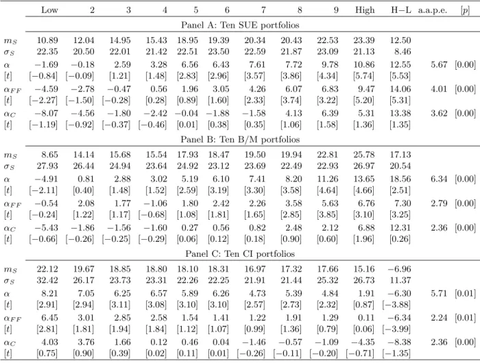
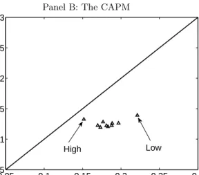
The SUE, B/M, and CI effects are well-known regularities that cannot be accounted for by traditional asset pricing models. Panel A of Table 1 show that from the low SUE to the high SUE portfolio the average return increases monotonically from 10.89% to 23.39% per annum. The portfolio volatilities are largely flat at around 22%. We estimate the CAPM and the Fama-French three-factor model using annual time series regressions. The intercept from the CAPM regression (“alpha” or “pricing error”) of the high-minus-low SUE portfolio is 12.55% per annum (t = 5.53), and the average absolute value of the pricing errors, denoted a.a.p.e., is 5.67%. The Gibbons, Ross, and Shanken (1989, GRS) statistic, which tests the null hypothesis that all the individual alphas are jointly zero, rejects the CAPM. The alphas do not add up to zero because we equal-weight the testing portfolio returns. The performance of the Fama-French model is similar: the a.a.p.e. is 4.01% and the GRS test rejects the model. The intercept from the Fama-French three-factor regression (“Fama-French alpha”) of the high-minus-low SUE portfolio is 14.06% per annum (t= 5.31).

We also estimate the standard consumption CAPM with the CRRA utility based pricing kernel,

mt+1=β(ct+1/ct)−γ, in whichβ is time preference coefficient andγ is risk aversion. Consumption,

ct, is annual per capita consumption of nondurables and services from the Bureau of Economic Analysis. We use one-stage GMM with the identity weighting matrix to estimate the moments

E[mt+1(rStj +1−rf t+1)] = 0, in whichrf t+1is the annualized return on the one-month Treasury bill

from Ibbotson Associates. We also include E[mt+1rf t+1] = 1 as an additional moment condition

to identify β. We calculate the consumption alpha,αj_C, as E[mt+1(rjSt+1−rf t+1)]/E[mt+1].

The consumption CAPM cannot capture the SUE effect. From Panel A of Table 1, the con-sumption alpha increases from−8.07% for the low SUE portfolio to 5.13% per annum for the high

SUE portfolio. The difference of 13.38% is economically large. Although the alphas are not in-dividually significant, probably because of large measurement errors in consumption data, the χ2

the parameter estimates are unrealistic: the estimate of the time preference coefficient is 2.76, and estimate of the risk aversion parameter is 127.59.

Panel B of Table 1 shows that value stocks with high B/M ratios earn higher average stock returns than growth stocks with low B/M ratios, 25.78% vs. 8.65% per annum. The difference of 17.13% is significant (t = 5.53). There is no discernible relation between B/M and stock return volatility: both the value and the growth portfolios have volatilities around 27%. The CAPM alpha increases monotonically from −4.91% for growth stocks to 13.65% for value stocks. The average

magnitude of the alphas is 6.34% per annum and the GRS test strongly rejects the CAPM. Even the Fama-French model fails to capture the equal-weighted returns across the ten B/M portfolios: the high-minus-low B/M portfolio has a Fama-French alpha of 7.30% per annum (t= 3.25). The consumption alpha increases from −5.43% for growth stocks to 6.88% for value stocks with an

average magnitude of 2.36% per annum, and the consumption model is rejected by the χ2 test. From Panel C of Table 1, high CI stocks earn lower average stock returns than low CI stocks: 15.16% vs. 22.12%. The difference of −6.96% per annum is more than four standard errors from

zero. The volatilities of the low CI stocks are slightly higher than those of the high CI stocks: 32.42% vs. 26.73%. The high-minus-low CI portfolio has a CAPM alpha of −6.30% (t = −3.88)

and a Fama-French alpha of −6.34% (t = −3.99). Both models are rejected by the GRS test.

The consumption alpha decreases from 4.03% for the low CI portfolio to −4.35% for the high CI

portfolio with an average magnitude of 2.36% per annum, and theχ2 test rejects the model.

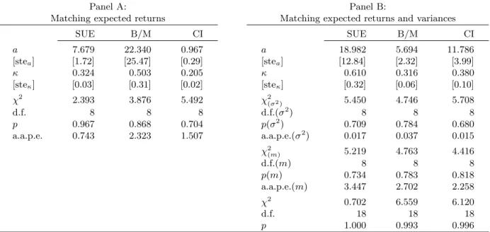
4.2 Matching Expected Returns

4.2.1 Point Estimates and Overall Model Performance

We estimate only two parameters in our parsimonious model: the adjustment cost parameter, a,

and capital’s share, κ. Panel A of Table 2 provides estimates of κ that are often significant and that range from 0.21 to 0.50. These estimates are reasonably close to the approximate 0.30 figure for capital’s share used in Rotemberg and Woodford (1992, 1999). The estimates of a are not as stable across the different sets of testing portfolios. We find significant estimates of 7.68 and 0.97 for the SUE and CI portfolios, respectively. The estimate is 22.34 for the B/M portfolios but with a high standard error of 25.47. Although some of these estimates ofaare large, they fall within the wide range of estimates from studies using quantity data (e.g., Summers 1981 and Whited 1992). Finally, the evidence implies that firm’s optimization problem has an interior solution because the positive estimates ofamean that the adjustment cost function is increasing and convex inij_t.

Panel A also reports two measures of overall model performance: the average absolute pricing error, a.a.p.e., and theχ2 test. The model performs quite well in accounting for the average returns of the ten SUE portfolios. The a.a.p.e. is 0.74% per annum, which is much lower than those from the CAPM, 5.67%, the Fama-French model, 4.01%, and the consumption CAPM, 3.62%. Unlike the traditional models that are rejected using the SUE portfolios, our model is not rejected by the

χ2 test. The overall performance of our model is more modest in accounting for the average returns of the ten B/M portfolios. Although the model is not formally rejected by theχ2test, the a.a.p.e. is 2.32% per annum, which is comparable to that from the Fama-French model, 2.79%, and that from the consumption CAPM, 2.36%, but is lower than that from the CAPM, 6.34%. The investment model does better in pricing the ten CI portfolios. The a.a.p.e. is 1.51% per annum, which is lower than those from the CAPM, 5.71%, the Fama-French model, 2.24%, and the consumption CAPM, 2.36%. Once again, our model is not rejected by theχ2 _test.

4.2.2 Euler Equation Errors

The average absolute pricing errors and χ2 tests only indicate overall model performance. To provide a more complete picture, we report for each portfolio its individual error, defined as

ejm≡E

h

r_Stj ₊₁−LrjIt+1

i

, in whichLrItj+1 is constructed using the estimates from Panel A of Table

2. We also report thet-statistic, described in Appendix B, testing thatejmfor portfoliojequals zero. Panel A of Table 3 reports the individual average return errors or mean errors. The magnitude of ejm varies from 0.05% to 1.72% per annum across the ten SUE portfolios. None of the mean errors are significant. In particular, the high-minus-low SUE portfolio has a mean error of −0.40%

per annum (t= −0.34), which is negligible compared to the significant errors from the traditional

models that range from 12.55% to 14.06% per annum.

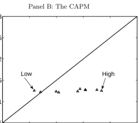
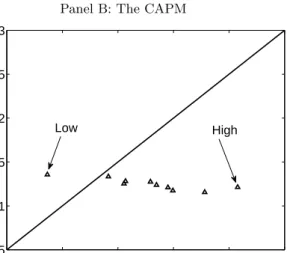
Figure 1 provides a visual presentation of the fit. Panel A plots the average levered investment returns of the ten SUE portfolios against their average stock returns. If the model performs per-fectly, all the observations should lie precisely on the 45-degree line. Panel A shows that the scatter plot from the investment model is closely aligned with the 45-degree line. The remaining panels contain analogous plots for the CAPM, the Fama-French model, and the consumption CAPM. In all three cases the scatter plot is largely horizontal, meaning that the traditional models almost completely fail to predict the average returns across the SUE portfolios.

Moving to the B/M portfolios, we observe relatively large mean errors in Panel A of Table 3. Three out of ten portfolios have mean errors with magnitudes higher than 3% per annum and six

out of ten have mean errors with magnitudes higher than 2.5%. The growth portfolio has a mean error of−3.94%. However, the mean errors in our model do not vary systematically with B/M. The

high-minus-low B/M portfolio only has a mean error of 1.21% per annum, which is substantially smaller than 12.31% in the consumption CAPM and 7.30% in the Fama-French model. The scatter plots in Figure 2 show that, although the model errors from the investment model are largely sim-ilar in magnitude to those from the Fama-French model and the consumption CAPM, the average return spread between the low and the high B/M portfolios from our model is much larger than the spreads from the traditional models.

From Panel A of Table 3, the mean errors from the CI portfolios are somewhat larger than those from the SUE portfolios but are much smaller than those from the B/M portfolios. Only three out of the ten CI portfolios have mean errors larger than 2.5% per annum. The high-minus-low CI portfolio has a small mean error of −0.49% (t = −0.43), meaning that the investment model

generates a realistic average return spread across the two extreme CI portfolios. The scatter plot in Panel A of Figure 3 confirms this observation. In contrast, none of the traditional models are able to reproduce the average return spread, as shown in the rest of Figure 3.

4.2.3 Expected Return Accounting

To understand the economic forces driving our estimation results, we examine the patterns across the testing portfolios of the characteristics that make up levered investment returns. Equation (13) says that, all else equal, firms with high investment-to-capital today should earn lower aver-age returns than firms with low investment-to-capital today. Firms with high future investment growth should earn higher average returns than firms with low future investment growth. Firms with high to-capital tomorrow should earn higher average returns than firms with low sales-to-capital tomorrow. Collecting terms involving δj_t+1 in the numerator of equation (13) yields

−(1−τt+1)[1 +a(ijt+1/k

j t+1)]δ

j

t+1, meaning that high rates of depreciation tomorrow imply lower

average returns. Finally, taking the first-order derivative of equation (16) with respect toνj_t shows that the expected stock return should increase with market leverage today.

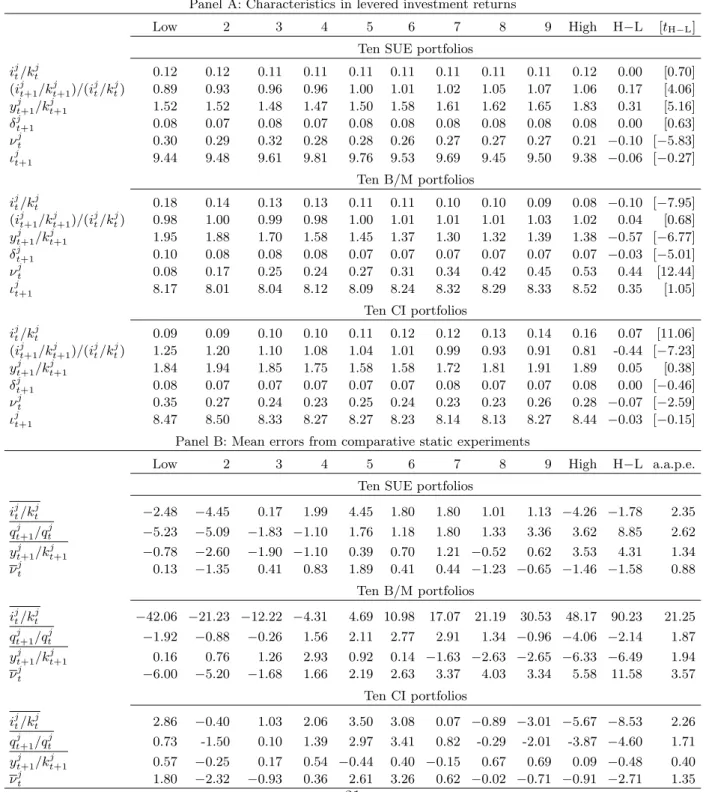
Table 4 presents averages of firm characteristics across our testing portfolios. Panel A shows that the averages ofij_t/kj_t, δj_t+1, and the bond returns are largely flat across the ten SUE portfolios. The averages ofij_t+1/k_tj₊₁/i_tj/kj_t(future investment growth) andyj_t+1/kj_t+1 both increase from the low SUE portfolio to the high SUE portfolio, going in the right direction for capturing average stock returns. However, going in the wrong direction, market leverage decreases from the low to the

high SUE portfolio. In the case of the B/M portfolios,ij_t/k_tj decreases from 18% to 8% per annum from the low to the high portfolio. The low B/M firms also have higher rates of depreciation (10% vs. 7%) and lower leverage (8% vs. 53%) than the high B/M firms. All three characteristics go in the right direction for matching average stock returns. However, going in the wrong direction, the low B/M firms have higher average y_tj₊₁/k_tj₊₁ (1.95 vs. 1.38) than the high B/M firms. Average bond returns and investment growth are roughly flat across the B/M portfolios. Not surprisingly, sorting on CI produces a large spread inij_t/kj_t of 7.3%. This characteristic increases monotonically from 9% for the low to 16% for the high CI portfolio. Compared to the high CI firms, the low CI firms also have much higher future investment growth (1.25 vs. 0.81) and higher market leverage (35% vs. 28%). All three patterns go in the right direction for matching average stock returns. The remaining characteristics are largely flat across the CI portfolios.

The observed patterns in these characteristics help explain the differences in the estimates of the adjustment cost parameter, a, across the different sets of portfolios. In the case of the B/M portfolios, for example, the characteristicy_tj₊₁/kj_t+1 goes strongly in the wrong direction for match-ing average stock returns. Equation (13) suggests that this backward cross-sectional movement in the numerator of the investment return must be countered with a relatively strong movement in the denominator if average estimated levered investment returns are to match average stock returns. A high estimate of a(22.3) accomplishes this goal by magnifying the movement in the denominator. For the CI portfolios both future investment growth and ij_t/kj_t go strongly in the right direction. The magnifying effect of a (0.967) therefore does not need to be large to minimize the pricing errors. The cross-sectional movement in ij_t/k_tj for the SUE portfolios is negligible, meaning that the parameteraonly operates via its effect on future investment growth. The estimate of 7.6 falls between the extreme estimates for the other testing portfolios.

To quantify the importance of each characteristic for driving expected stock returns, we conduct the following expected return accounting exercises. We start with the parameters re-ported in Panel A of Table 2. We set a given characteristic equal to its cross-sectional av-erage in each year. We then use the estimated parameters to reconstruct the levered invest-ment returns, while keeping all the other characteristics unchanged. In the case of future in-vestment growth we hold constant the capital gain component of the inin-vestment return given by

h

1 + (1−τt+1)a

ij_t+1/k_tj₊₁i. h1 + (1−τt)a

ij_t/k_tji=q_tj₊₁/q_tj, and allow all other components to vary. We focus on the resulting change in the magnitude of the mean errors: a large change

would suggest the quantitative importance for the characteristic in question.

Panel B of Table 4 reports several insights. First, the most important characteristic in driving the SUE portfolio returns is q_tj₊₁/q_tj: eliminating its cross-sectional variation makes our model underpredict the average stock return of the high-minus-low SUE portfolio by a mean error of 8.85% per annum. In contrast, this error is only−0.40% in Table 3. ytj+1/k

j

t+1 also is important: without

its cross-sectional variation, the mean error of the high-minus-low SUE portfolio becomes 4.31%. Second, investment and leverage are both important for the B/M portfolios. Fixingij_t/k_tj to its cross-sectional average produces a mean error of 90.23% per annum for the high-minus-low B/M portfolio. This huge error largely reflects the large estimate of the coefficient afor this set of test-ing portfolios. Setttest-ing νj_t to its cross-sectional average produces a mean error of 11.58% for the high-minus-low B/M portfolio. y_tj₊₁/k_tj₊₁ and qj_t+1/qj_t also play a role, but they are quantitatively less important thanνj_t. Third, the dominating force in driving the average stock returns across the CI portfolios isij_t/k_tj. Eliminating its cross-sectional variation gives rise to a mean error of−8.53%

per annum for the high-minus-low CI portfolio. Fixingqj_t+1/qj_t in the cross section produces a sub-stantial mean error of 4.6%, andνj_t contributes 2.7% per year. The effect ofyj_t+1/kj_t+1 is negligible.

4.3 Matching Expected Returns and Variances

To preview the results, when used to match both expected returns and variances, our model matches the variances but leaves large errors in the mean returns.

4.3.1 Point Estimates and Overall Model Performance

Panel B of Table 2 reports the point estimates and overall model performance when we use the investment model to match both the expected returns and variances of the testing portfolios. Cap-ital’s share, κ, is estimated from 0.32 to 0.61, and all estimates are significant. The estimates of the adjustment cost parameter, a, are on average higher than those reported in Panel A, and are more stable across the different testing portfolios. The estimates are 2.32 and 11.76 for the B/M and CI portfolios, and both estimates are significant. The estimate ofa for the SUE portfolios is 18.98, but with a large standard error of 12.84.

Panel B reports three tests of overall model performance. χ2

(σ2₎is theχ2test that all the variance

errors are jointly zero,χ2_(m)is theχ2test that all the mean errors are jointly zero, and the statistic la-beledχ2_{tests that all the mean and variance errors are jointly zero. Theχ}2

(σ2₎tests do not reject the

To understand its economic magnitude, we use the parameter estimates from Table 2 to calculate the average leveraged investment return volatility (instead of variance). At 18.1%, this predicted volatil-ity is close to the average realized volatilvolatil-ity 21.1% across the ten SUE portfolios. For the B/M port-folios, a.a.p.e.(σ2_{) is 0.037, which is somewhat large relative to the average stock return volatility of}

25%. For comparison, the average levered investment return volatility across the ten B/M portfolios is 18.6%. Finally, for the ten CI portfolios a.a.p.e.(σ2) is 0.017, which is small relative to their aver-age stock return volatility of 24.8% and their averaver-age levered investment return volatility of 22.6%. Although theχ2_(m)tests on the mean errors do not reject the model, the magnitudes of the mean errors, denoted a.a.p.e.(m), are relatively large. The a.a.p.e.(m) for the SUE portfolios is 3.45% per annum, up from 0.74% when matching expected returns only. The a.a.p.e.(m) for the B/M portfolios actually falls slightly from 2.32% to 2.26%, while that for the CI portfolios goes up from 1.51% to 2.70%. Finally, the χ2 _{tests fail to reject the model probably because of measurement}

errors in quantity data. As such, we only focus on the magnitude of the mean and variance errors. Our volatility results complement those in Cochrane (1991) in several ways. First, we account for leverage, while Cochrane does not. Second, we use portfolios formed on firm characteristics as testing assets, in which firm-specific shocks are unlikely to be completely diversified away, while Cochrane studies the stock market portfolio. Third, and most important, we formally choose pa-rameters to match volatilities. In contrast, Cochrane calibrates his papa-rameters to match average returns perfectly, while letting volatilities vary freely.6

4.3.2 Euler Equation Errors

To provide a more complete picture of the model’s performance, Panel B of Table 3 reports in-dividual variance errors, defined as ej_σ2 ≡ σ2

r_Stj ₊₁−σ2

LrItj+1

, and mean errors, defined as

ejm≡E

h

r_Stj ₊₁−Lrj_It+1

i

, in whichLr_Itj₊₁ is constructed using the estimates from Panel B of Table 2. Their t-statistics are calculated using the variance-covariance matrix from one-stage GMM.

Panel B of Table 3 shows that with a few exceptions, the magnitude of the variance errors is small relative to the level of stock return variances. Most variance errors are insignificant. The left panels in Figure 4 plot levered investment return volatilities against stock return volatilities for the testing portfolios. To facilitate interpretation, we plot volatilities instead of variances. The points in the scatter plot are generally aligned with the 45-degree line. However, while there is no

6_{Israelsen (2008) shows that levered aggregate investment returns are as volatile as stock market returns after} incor-porating investment-specific technological progress and non-quadratic adjustment costs into theq-theory framework.

discernible relation between stock return volatilities and the characteristics in the data, the model seems to predict a negative relation between levered investment return volatilities and SUE (Panel A) and a positive relation between the predicted volatilities and B/M (Panel C). Panel B of Table 3 shows that the variance errors seem to increase with SUE and decrease with B/M and CI. For example, the difference in the variance errors between the high and low SUE portfolios is 0.046, and the difference between the high and low B/M portfolios is−0.128. The difference in variance

errors is only significant, however, for the B/M portfolios.

Panel B of Table 3 shows that the mean errors vary systematically with SUE:ejm increases from

−7.02% per annum for the low SUE portfolio to 5.37% for the high SUE portfolio. The difference of

12.39% (t= 2.50) is similar in magnitude to those from the traditional models. Panel B of Figure 4 plots the average levered investment returns against the average stock returns. The pattern is largely horizontal, similar to those from the traditional models. The mean errors for the B/M portfolios in Panel B of Table 3 also are larger than those from Panel A, which come from matching only expected returns. However, the model still predicts an average return spread of 10% per annum between the two extreme B/M portfolios. The mean error for the high-minus-low B/M portfolio is 7.11% per annum in the investment model, which is lower than 7.30% from the Fama-French model. The CAPM and consumption CAPM produce even higher mean errors, 18.56% and 12.31%, respectively. The model’s performance in reproducing the average returns of the CI portfolios deteriorates to the same level as in the traditional models. The mean error difference between the high and low CI portfolios is −6.51%, which is similar to those from the CAPM and the

Fama-French model. From Panel F of Figure 4, the scatter plots of average returns from the investment model are largely horizontal, similar to the patterns reported in Figure 3 for the traditional models.

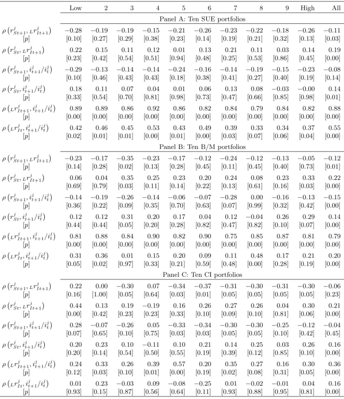
4.3.3 A Correlation Puzzle

As noted, equation (16), taken literally, predicts that stock returns should equal levered investment returns at every data point. To derive economically meaningful tests, we have so far examined the first and second moments of returns that are the focus of much work in empirical finance. We can explore yet another (strong) prediction of the model: stock returns should be perfectly correlated with levered investment returns. Table 5 reports time series correlations between the two types of returns for each testing portfolio. The contemporaneous correlations are weakly negative, while the correlations between one-period-lagged stock returns and levered investment returns are positive. For example, when we pool all the observations in the SUE portfolios together, the

contempora-neous correlation is −0.11 (p = 0.03). However, the correlation between one-period-lagged stock

returns and levered investment returns is 0.19 (p = 0.00). Replacing levered investment returns with investment growth yields similar results, meaning that the correlations are insensitive to speci-fication errors in the investment returns. Table 5 also shows that, in contrast to the weakly negative correlations between stock returns and investment growth, the model predicts counterfactually high correlations between levered investment returns and investment growth.

The evidence suggests that investment lags are more important for reproducing the correlation structure between stock returns and investment growth than for means and volatilities of returns. At the aggregate level, Cochrane (1991) reports a high contemporaneous correlation between stock returns and investment growth. Our evidence suggests that investment lags seem to be more important at a more disaggregated level.7 However, incorporating investment lags into the model to address the correlation puzzle is beyond our scope. As noted, investment lags appear less important for the first and potentially even the second moments of returns that we focus on in this paper. Incorporating investment lags will likely only improve the fit along these two crucial dimensions.

5

Summary and Future Work

We use GMM to estimate a structural model of cross-sectional stock returns derived from the q -theory of investment. We construct empirical first and second moment conditions based on the

q-theory prediction that stock returns equal levered investment returns, the latter of which are observable because they are functions of firm characteristics. Our parsimonious model (with only two parameters) goes a long way toward capturing the average stock returns of portfolios formed on earnings surprises, book-to-market, and capital investment. The volatilities from the model also are empirically plausible. However, the model falls short in matching expected returns and volatilities simultaneously and in reproducing the correlation structure between stock returns and investment growth. In addition, because we avoid the parametrization of the stochastic discount factor, our model is silent about why average return spreads across characteristics-sorted portfolios are not matched with spreads in covariances. In sum, we interpret our results as saying that on average portfolios of firms do a good job of aligning investment policies with their costs of capital, and that this alignment drives many observed correlations between stock returns and firm characteristics.

7_{Israelsen (2008) shows that Cochrane’s (1991) result is driven by equipment investment growth and that the} correlation between stock returns and structure investment growth is weakly negative. Intuitively, investment lags that arise from, for example, time-to-plan and time-to-build, are more applicable to structures than to equipment.

We view our contribution as mainly providing a simple structure that links the cross section of returns to characteristics in an economically interpretable way. To preserve the transparency of the economic mechanisms that drive our results, we have not searched deliberately for alternative specifications to maximize the model fit. This simplicity leaves open many paths for extending the model. One can introduce capital heterogeneity, labor adjustment costs, costly reversibility, flow fixed costs of production or investment, financing constraints, investment-specific technological shocks, and non-quadratic adjustment costs, while preserving the closed-form Euler equation tests. Decreasing returns to scale, investment lags, and pure fixed costs can be incorporated as well. How-ever, the analytical link between stock and investment returns breaks, and the resulting models can only be estimated via Simulated Method of Moments. Not only can our framework be extended in terms of modeling, but it can be used to understand the many statistical relations in empirical finance that call for theoretical insights. These relations include those between average stock re-turns and prior stock rere-turns, new equity issues, financial distress, liquidity, idiosyncratic volatility, corporate governance, and accounting accruals (the difference between earnings and cash flows). Finally, the asset pricing literature on corporate bonds has traditionally built on the contingent-claims framework with exogenous investment and cash flows. Taking stock returns as given, one can turn equation (15) around as a theory for corporate bond returns. A dynamic trade-off theory of optimal capital structure can be embedded into our framework. Doing so provides a more complete description of the relations between leverage and expected stock and bond returns.

References

Abel, Andrew B. and Janice C. Eberly, 1994, A unified model of investment under uncertainty,

American Economic Review 84 (1), 1369–1384.

Abel, Andrew B. and Janice C. Eberly, 2001, Investment and q with fixed costs: An empirical analysis, working paper, The Wharton School, University of Pennsylvania.

Ball, Ray and Philip Brown, 1968, An empirical evaluation of accounting income numbers,Journal of Accounting Research 6, 159–178.

Berk, Jonathan B. and Peter DeMarzo, 2007, Corporate Finance, Pearson Education, Inc. Berk, Jonathan B., Richard C. Green, and Vasant Naik, 1999, Optimal investment, growth options,

and security returns,Journal of Finance, 54, 1153–1607.

Bernanke, Ben S. and John Y. Campbell, 1988, Is there a corporate debt crisis? Brookings Papers on Economic Activity 1, 83–125.

Blume, Marshall E., Felix Lim, and A. Craig MacKinlay, 1998, The declining credit quality of U.S. corporate debt: Myth or reality? Journal of Finance 53 (3), 1389–1413.

Brainard, William C., and James Tobin, 1968, Pitfalls in financial model building, American Economic Review 58 (2), 99–122.

Carlson, Murray, Adlai Fisher, and Ron Giammarino, 2004, Corporate investment and asset price dynamics: Implications for the cross section of returns,Journal of Finance 59 (6), 2577–2603. Chan, Louis K. C., Narasimhan Jegadeesh, and Josef Lakonishok, 1996, Momentum strategies,

Journal of Finance, 51 (5), 1681–1713.

Chincarini, Ludwig B. and Daehwan Kim, 2006, Quantitative equity portfolio management: An active approach to portfolio construction and management, McGraw-Hill.

Cochrane, John H., 1991, Production-based asset pricing and the link between stock returns and economic fluctuations, Journal of Finance 46, 209–237.

Cochrane, John H., 1996, A cross-sectional test of an investment-based asset pricing model,

Journal of Political Economy 104, 572–621.

Dimson, Elroy, 1979, Risk management when shares are subject to infrequent trading, Journal of Financial Economics 7, 197–226.

Eberly, Janice, Sergio Rebelo, and Nicolas Vincent, 2008, Investment and value: A neoclassical benchmark, working paper, Northwestern University.

Erickson, Timothy, and Toni M. Whited, 2000, Measurement error and the relationship between investment and q, Journal of Political Economy 108 (5), 1027–1057.

Erickson, Timothy, and Toni M. Whited, 2006, On the Accuracy of Different Measures of Q,

Financial Management 35, 5–33.

Fama, Eugene F., 1998, Market efficiency, long-term returns, and behavioral finance, Journal of Financial Economics 49, 283–306.

Fama, Eugene F. and Kenneth R. French, 1993, Common risk factors in the returns on stocks and bonds,Journal of Financial Economics 33, 3–56.

Fama, Eugene F. and Kenneth R. French, 1995, Size and book-to-market factors in earnings and returns,Journal of Finance 50, 131–155.

Gibbons, Michael R., Stephen A. Ross, and Jay Shanken, 1989, A test of the efficiency of a given portfolio, Econometrica 57 (5), 1121–1152.

Graham, John R., 1996, Proxies for the corporate marginal tax rate, Journal of Financial Economics 42, 187–221.

Graham, John R., 2003, Taxes and corporate finance: A review, Review of Financial Studies 16 (4), 1075–1129.

Hall, Robert E., 2004, Measuring factor adjustment costs, Quarterly Journal of Economics 119 (3), 899–927.

Hall, Robert E. and Dale W. Jorgenson, 1967, Tax policy and investment behavior, American Economic Review 57, 391–414.

Hansen, Lars Peter, 1982, Large sample properties of generalized method of moments estimators,

Econometrica 40, 1029–1054.

Hansen, Lars Peter and Kenneth J. Singleton, 1982, Generalized instrumental variables estimation of nonlinear rational expectations models, Econometrica 50, 1269–1288.

Hayashi, Fumio, 1982, Tobin’s marginal and average q: A neoclassical interpretation,

Econometrica 50 (1), 213–224.

Hennessy, Christopher A. and Toni M. Whited, 2007, How costly is external financing? Evidence from a structural estimation,Journal of Finance 62 (4), 1705–1745.

Hubbard, Glenn R., Anil K. Kashyap, Toni M. Whited, 1995, Internal finance and firm investment,

Journal of Money, Credit, and Banking 27 (3), 683–701.

Israelsen, Ryan D., 2008, Investment based valuation, Working paper, Stephen M. Ross School of Business, University of Michigan.

Lettau, Martin and Sydney C. Ludvigson, 2001, Resurrecting the (C)CAPM: A cross-sectional test when risk premia are time-varying, Journal of Political Economy 109, 1238–1287. Love, Inessa, 2003, Financial development and financial constraints: International evidence from

the structural investment model, Review of Financial Studies 16 (3), 765–791.

Lucas, Robert E. Jr. and Edward C. Prescott, 1971, Investment under uncertainty, Econometrica

39, 659–681.

Philippon, Thomas, 2008, The bond market’sq, forthcoming,Quarterly Journal of Economics. Restoy, Fernando and G. Michael Rockinger, 1994, On stock market returns and returns on

investment,Journal of Finance 49 (2), 543–556.

Rotemberg, Julio J. and Michael Woodford, 1992, Oligopolistic pricing and the effects of aggregate demand on economic activity, Journal of Political Economy 100, 1153–1207.