Load Balancing Algorithms for Sparse Matrix Kernels on Heterogeneous Platforms

(1)

Load Balancing Algorithms for Sparse Matrix Kernels on Heterogeneous

Platforms

Thesis submitted in partial fulfillment of the requirements for the degree of

MS by Research in

Computer Science and Engineering

by

I Shiva Rama Krishna 201007002

[email protected]

International Institute of Information Technology Hyderabad - 500 032, INDIA

(2)

(3)

International Institute of Information Technology

Hyderabad, India

CERTIFICATE

It is certified that the work contained in this thesis, titled “Load Balancing Algorithms for Sparse Ma-trix Kernels on Heterogeneous Platforms ” by I Siva Rama Krishna, has been carried out under my supervision and is not submitted elsewhere for a degree.

(4)

(5)

Acknowledgments

First I would like to thank Dr. Kishore Kothapalli for all the support, guidance, suggestions and encouragement. He is a wonderful guide and supported me with his patience and his knowledge. He patiently listened to what ever I say and helped me to think in right direction when i was stuck. I am really thankful to him for being available to me even during odd hours.

I am grateful to CSTAR for providing enough resources and nice atmosphere for doing research. I would like to thank my lab mates, Jatin, Kiran, Dip sankar banerjee, Anil kishore, Aman, Shashank, Manoj, Piyush, Ravi kishore, Chiranjeevi for their support and encouragement. Special thanks to Anil kishore for his simplicity and encouragement and to Kiran for his support, guidance and encouragement. I am really thankful to my friends Nikhil, Vikram, Jatin, Ruchi for their love and support when I was having tough time. Special thanks to harsh for enlightening me about various issues. I will cherish all the memories for rest of life.

Finally and most importantly, I would like to thank my parents for their unconditional love and support throughout the thesis.

(6)

Abstract

After microprocessor clock speeds have levelled off, high performance community started using GPU (graphics processing unit) for general purpose computing. This is because of their performance per unit cost, performance per unit watt and CUDA programming model. So it is not surprising that most of top super computers use GPU as one of their computing element [56]. As GPU’s architecture is different , to get good performance using GPU, we need to reinterpret the application in highly multi-threaded manner. GPUs are good at exploiting massive data parallelism and they are well suited for applications which has regular memory access patterns. This can be observed in many applications such as scan primitives [57], sort [52], dense matrix multiplication [15]. However most of the applications in high performance computing are irregular in nature. GPUs are not well suited for irregular applications such as graph algorithms [16], sparse matrix operations [45], list ranking [27] etc.

GPU is not a standalone device and it needs a host device like CPU. In a normal GPU application, CPU sits idle while GPU is doing the computation. So it is beneficial to include the CPU in computation. We call it asheterogeneous computing. This kind of effort was done in recent works such as dense linear algebra computations [60], sorting [29], list ranking [31].

Sparse matrix operations are some of fundamental problems in parallel computing. It is included in the seven dwarfs of parallel computing identified in the Berkely report [3]. In this thesis we design heterogeneous algorithms for sparse matrix operations such as sparse matrix - vector multiplication (spmv), sparse matrix - sparse matrix multiplication (spgemm) and sparse matrix - dense matrix mul-tiplication (csrmm). The fundamental problem inheterogeneous computingis partitioning the work among devices. So we explore different work division methodologies.

We first designedstatic load balancing algorithms for these sparse matrix operations. Later we proposed adynamic load balancingalgorithm using a work queue and studied the efficacy of it using sparse matrix operations. We also propose a analytical model to divide work in case of band matrix multiplication. We noticed that theheterogeneous computing is suitable for irregular applications such as sparse matrix operations. Ourstatic load balancingalgorithm ofspgemm,csrmm,spmv are 30%, 15%, 20% faster compared to their pure GPU solutions respectively. We also show that for scale free matrices, inspmv operation, giving large rows to CPU and small rows to GPU is most suitable work division scheme. We verified the efficacy of ourdynamic load balancing algorithm on two different heterogeneous platforms usingspgemm andcsrmm. We show that the absolute difference of work division percentages and execution times with respect tostatic load balancing approach are

(7)

vii under 6% and 10% respectively. Also in case of band matrix multiplication, our proposed analytical method is able to predict the best work division percentage at accuracy more than 95%.

(8)

List of Figures

Figure Page

1.1 tightly coupled cpu-gpu heterogenous platform . . . 2 2.1 Different sparse matrix representations for an example matrix . . . 10 2.2 The specifications for the different GPUs and CPUs used in our experiments. . . 13 2.3 List of sparse matrices. Number of columns and rows are equal for all the matrices

except for the matrix LP, where the number of columns is equal to1,092,610. . . 14 2.4 List of sparse matrices from SNAP dataset . . . 15 3.1 spgemm using static load balancing. The red colored rows are processed on CPU and

blue colored rows are processed on GPU. . . 17 3.2 Performance comparison of heterogeneous method w.r.t Row-Row method on datasets

shown in Figure 2.3, Figure 2.4 on Hetero-II given in Section 2.5.2. . . 18 3.3 Performance comparison of two presented heuristics w.r.t the best heterogeneous

tim-ings on the dataset shown in Figure 2.3 on platform Hetero-II given in Section 2.5.2. X-axis represents instances in dataset and Y-axis represents performance w.r.t best het-erogeneous time. The last instanceAverageshows the average value of the series. . . . 20 3.4 Performance comparison of heterogeneous algorithm w.r.t GPU algorithm forcsrmm[48]

on dataset shown in Figure 2.3 on the Hetero-I given in Section 2.5.1. . . 21 3.5 Figure shows the Direct-Division scheme for spmv. The red colored rows of A are

processed on the CPU, and the other rows are processed on the GPU. The corresponding portion of the result vector in each iteration is also colored accordingly. . . 23 3.6 Figure shows the Large-Rows-GPU scheme forspmv. The red colored rows ofAare

processed on the CPU, and the other rows are processed on the GPU. The corresponding portion of the result vector in each iteration is also colored accordingly. . . 24 3.7 Figure shows the Small-Rows-GPU scheme forspmv. The red colored rows ofAare

processed on the CPU, and the other rows are processed on the GPU. The corresponding portion of the result vector in each iteration is also colored accordingly. . . 24 3.8 Performance comparison of execution times of the three work division methods for

sparse matrices from two different datasets on platform given in 2.5.1. The line an-chored to the second Y-axis, labeled Max/Min, measures the ratio of the best speed-up to the least speed-up among the three work division methods. The last item on the X-axis refers to the average of the dataset. . . 26

(11)

LIST OF FIGURES xi

3.9 Figure showing the timeline of two iterations ofspmv on the matrix FEM/Cantilever from Table 2.3. The labels CPU and GPU indicate computations on the CPU and the GPU respectively. The labels CPU→ GPU and GPU→ CPU indicate transfer of the partial result vector from the CPU to the GPU and vice-versa. . . 27 3.10 Applying the Small-Rows-GPU method to scale-free matrices from the datasets of Table

2.3 and 2.4 on platform given in 2.5.1. The last item on the X-axis refers to the average of the series. . . 29 3.11 Cache hit ratio on the CPU last level cache for four different scale-free matrices. The

X-axis indicates the percentage of the total number of non-zeros that were assigned to the CPU. . . 30 4.1 Work Queue model . . . 32 4.2 Figure shows the absolute difference in the work split percentage with respect to the

baseline implementation for spgemm on platforms given in Sections 2.5.1(Hetero-High), 2.5.3(Hetero-Low). The last instance ”Average” shows the average value of the series. . . 35 4.3 Figure shows the absolute difference in the work split percentage with respect to the

baseline implementation forcsrmm on platforms given in Sections 2.5.1(Hetero-High), 2.5.3(Hetero-Low). The last instance ”Average” shows the average value of the series. 36 4.4 Figure shows the absolute difference in the runtime with respect to the baseline

imple-mentation forspgemm on platforms given in Sections 2.5.1(Hetero-High), 2.5.3(Hetero-Low). The last instance ”Average” shows the average value of the series. . . 37 4.5 Figure shows the absolute difference in the runtime with respect to the baseline

imple-mentation forcsrmm on platforms given in Sections 2.5.1(Hetero-High), 2.5.3(Hetero-Low). The last instance ”Average” shows the average value of the series. . . 38 4.6 Absolute difference of work division percentage and the overall runtime between the

work queue based algorithm and the baseline algorithm for scale-free matrices from Table 2.3 and Table 2.4 on platform given in Section 2.5.1. . . 42 5.1 An example illustrating DIA format representation . . . 44 5.2 Graph showing the performance comparison of best time, predicted time using

formu-lae, for various combinations ofAr,Ad, andBd. A tuplehl, m, niin the x-axis indicates

(12)

List of Tables

(13)

Chapter 1

Introduction

Sparse matrix is a special kind of matrix in which most of the entries are zeros. Sparse matrix operations are some of fundamental problems in parallel computing. It is included in the seven dwarfs of parallel computing identified in the Berkely report [3]. Because of their importance these operations are included in various libraries such as Intel MKL [42], Nvidia cusp [51] and cusparse [13]. Sparse matrix operations are also considered as important kernels in the class of throughput oriented applications [14]. As many entries are zeros in sparse matrices, separate storage formats are used where only the non-zero entries are stored. Implementing sparse matrix operations on modern architectures such as GPU is challenging for various reasons. Due to variations in the sparsity nature of the matrices, these operations pose severe load balancing problems amongst threads and irregular memory access patterns. So most of the work focuses on designing efficient heterogeneous algorithms for sparse matrix operations.

1.1

Relevance of Parallel Computing

Parallel computing has been in practice for the past several decades in supercomputing. But it became mainstream after the slowdown in frequency scaling and memory speeds due to physical constraints. General purpose processors became multi-core and there has been renowned interest in hardware accel-erators such GPUs, FPGAs and so on. In recent years, accelerator-based computing using accelaccel-erators such as the IBM Cell SPUs, FPGAs, GPUs, and ASICs has achieved clear performance gains compared to CPUs. Several challenging problems from parallel computing such as sorting [52], graph traversals [54], and the like are already known to have highly efficient implementations on a variety of accelerators. A common model in all the above works is to delegate the entire computation to the accelerator.

Graphics processing units (GPUs) are generally used for graphics rendering. They are used as ac-celerator for graphics computations along with the main processor. GPUs are also used in a wide range of devices including laptops, personal computers, mobile phones, embedded systems and game con-soles. Graphics applications are highly parallel in nature. So they necessitate the GPU to be highly parallel architecture. GPUs also have very high bandwidth for efficient transfer of data among cores.

(14)

Figure 1.1tightly coupled cpu-gpu heterogenous platform

Because of these properties GPUs have drawn the attention of HPC community for general purpose calculations. Among the accelerators, GPUs have occupied a prominent place due to their low cost and high performance-per-watt ratio along with powerful programming models such as CUDA. For instance, for under $2000, one can buy a GPU which has 4 TFLOP computation power and more than 200 GB bandwidth while it requires 225 Watt of power.

However, GPU is not a stand alone device and should be attached to a host device like CPU. In most of the GPU applications, CPU passes the code and the data onto the GPU and gets back the results. CPU sits idle while GPU is doing the computation. So involving the CPU in computation makes the resource utilization efficient. We call it as heterogeneous computing. Recently Intel has crafted a hybrid chip which has FPGA and Xeon processor on same chip [10]. Further, it is anticipated that future generation commodity systems will naturally have a heterogeneous collection of computing devices including CPUs and other accelerators. This warrants the design and development ofheterogeneous algorithms that run on a commodity heterogeneous platform.

Designing a heterogeneous algorithm possesses several challenges such as reducing data transfers among devices, assigning right kind of work to devices and load balancing among devices. There have been recent efforts to design and develop heterogeneous algorithms for a variety of problems such as dense linear algebra computations [60], sorting [29], list ranking [31]. In this thesis, we investigate several load balancing techniques given in Section 1.3 on sparse matrix operation from Basic Linear Algebra Subprograms (BLAS) Level 2 and Level 3.

(15)

1.2

GPU Computation and CUDA Model

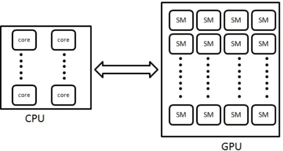
GPU is viewed as a massively multi-threaded architecture which has hundreds of small processing elements known ascores. Thesecoresare grouped in an SIMD fashion into a Streaming Multiprocessor (SM).

Using CUDA API, we can create a large number of threads to execute code on the GPU. All these threads are grouped intoblocksandblocksmake up agrid. Eachblockis further divided into SIMD groups calledwarps. Eachwarpconsists of up to 32 threads which execute the same instruction at any given time. During the execution time,blocksare serially scheduled on each SM. If ablockfinishes its computation the nextblockwill be scheduled. An SM can schedule multipleblocksat a time depending upon on theblocksize i.e, number of threads inblock. For instance, the GTX480 has 16 SMs and an SM can schedule two blocks ifblocksizeis 512. It means GTX480 can schedule 32 warps at a time. CUDA has zero over head scheduling when warps that are stalled on memory fetch are swapped with another warp. Data fetch latencies are hidden by switching betweenwarpsthat are resident on the SM.

The GPU has various types of memory. In a GPU each SM has an L1 cache orshared memory which is divided among theblocksthat are scheduled on the SM. In eachblocktheshared memory is shared by the threads in thatblock. Also each SM has 32 bitregisterswhich are divided among the threads scheduled on that SM. In general, all the private variables of a thread are stored in registers. In older GPUs, L1 cache is used only as a software managed cache. But in latest GPUs, some part of L1 cache is used as a hardware cache. Also new versions of GPUs have an L2 cache that services all load, store, and texture read/write requests. GPU also has off-chip memory known asglobal memorywhich is accessible to all the threads. We can efficiently accessglobal memorythrough two read-only caches known as theconstant memory andtexture memory. The constant memoryspace is cached on chip and it is used to store the constant data. So, one read memory request costs just one read from the constant cache if there is a cache hit, other wise it is one memory read from gloabal memory. T exture memoryis also cached on chip similar to constant memory. Specifically, texture caches are designed for graphics applications where memory access patterns has spatial locality. Typically the accesing times forglobal memoryandshared memoryare 400-600 and 20-40 cycles respectively.

Each computation that is to be performed using a GPU is written inside a module known askernels. Before we launch akernel, All the data needed by kernel should be transfered to GPU. Once the kernelis invoked from the CPU code, thekernelwill execute on GPU asynchronously with the CPU code. We do not have control on the scheduling ofblockson SM. Scheduling ofblockswill be taken care by the GPU. Also we do not have control on the execution or ordering of threads. All the threads in agridwork independently. We can keep barrier synchronization for all the threads in a block. Global synchronization among all the threads will be performed across separate kernel launches.

(16)

1.3

Load Balancing Strategies for Heterogeneous Platforms

In this section we give a brief explanation about the load balancing strategies used in this thesis.

1.3.1 Static Load Balancing

Static load balancing is a simple load balancing technique used in heterogeneous algorithms to partition the work among heterogeneous platforms. In this technique somet% of work is given to CPU and remaining work to GPU. But ’t’ is selected randomly before the start of computation. It has some drawbacks like partitioning the work irrespective of the instance leads to imbalance in the load. Because this partition method fails to capture any properties of a instance such as sparsity nature in case of matrices. Also for any instance it takes so much time to find best t% value as we need to find it through exhaustive experimentation. So we proposed anotherdynamic load balancingtechnique which is explained later.

Heterogeneous computing on commodity platforms is gaining large scale research attention in re-cent years. Heterogeneous algorithms have been designed rere-cently for several challenging problems in parallel computing including graph BFS [62, 48, 65], dense matrix computations [67], sorting [29], and the like. In the above cited works, they spread the entire computation across the computational devices. In some cases a post-processing phase is needed which combines the outputs of the individual compu-tations [31, 48, 29, 46, 60]. This approach of designing heterogeneous algorithms can be called as the static work partitioningorstatic load balancingapproach.

1.3.2 Dynamic Load Balancing

Dynamic load balancing is another simple load balancing strategy in which work is dynamically divided among heterogeneous devices. Static partitioning of work among heterogeneous platform has drawbacks such as partitioning irrespective of input instance cannot lead to well-balanced load. Finding best partitioning for a instance takes so much time as we have to search exhaustively. On the other hand analytical methods are available for special cases of workloads. Thus, a fundamental problem in heterogeneous computing is to propose generic mechanisms that can help address the issue of load balancing in heterogeneous algorithms designed using the work partitioning model[47]. So we proposed a light weight, low overhead, and completely dynamic load balancing framework that addresses the load balancing problem of heterogeneous algorithms. Details of our frame work is given in Chapter 4.

1.3.3 Analytical Model

In this strategy, we define a mathematical model using the parameters that effect the execution time. Using this model we find the work division threshold ’t’. But it is not always possible to design a analytical model for work division. Devising an analytical model reduces the exhaustive search time for

(17)

finding best work division threshold. In Chapter 5, we give details about the analytical model we used in this thesis.

1.4

Contributions

We investigate sparse matrix operations using different work division methodologies on different heterogeneous platforms. The contributions of this these are as follows

• We give an efficient heterogeneous algorithms for Sparse matrix - Sparse matrix multiplica-tion(spgemm), Sparse matrix - Dense matrix multiplication(csrmm) and Sparse matrix - Vector multiplication(spmv).

• Our static load balancing algorithms forspgemm,csrmm,spmv are 30%,15%,20% faster com-pared to GPU algorithms.

• We propose a dynamic work load balancing framework and used it to solve sparse matrix opera-tions on heterogeneous platform of CPU + GPU. The absolute difference of work split percentages and execution times with respect to static partitioning approach are under 6% and 10% respec-tively.

• We define an analytical model to identify correct work division among CPU and GPU in case of band matrix multiplication. We are able to predict correct work division percentage with an accuracy more than 95%.

(18)

Chapter 2

Background

This chapter has a brief explanation of different types of matrix multiplications, sparse matrix storage formats, sparse matrix operations, different load balancing algorithms for heterogeneous platforms and heterogeneous platforms which were used in this thesis.

2.1

Matrix Multiplication Formulations

LetA, B andC be three matrices with sizesM ×P, P ×N andM ×N respectively such that C =A×B. There are four different types of formulations to multiply two matrices. They are Row-Row formulation, Column-Row formulation, Row-Column formulation and Column-Column formulations. All these four formulations are briefly explained with an example.

2.1.1 The Row-Column Formulation

In the Row-Column formulation, to get one element inC, we multiply a row in theAmatrix with a column in theBmatrix, i.e.,C(i, j) =A(i,:)×B(:, j)fori= 1,2,· · ·, M, andj= 1,2,· · ·, N. This is the standard matrix multiplication approach. For a giveni,j, letI(i, j) denote the set of indicesk such that both the elementsA(i, k)andB(k, j)are nonzero. Then,C(i, j) =P

k∈I(i,j)A(i, k).B(k, j). However, to obtainI(i, j), we need to access all the elements in theithrow ofAandjthcolumn ofB. Therefore, we bring in elements which may not contribute to the output. In the worst case, we would access the entire row iofA and a columnj ofB whereasI(i, j) = Φ. Hence, this approach is not suited for sparse matrices in general.

2.1.2 The Row-Row Formulation

In the Row-Row formulation, to compute theith row in C, C(i,:), we multiply each element in A(i,:) with corresponding row in B. We then add all the scaled B rows to get the C(i,:). Thus, C(i,:) = P

j∈A(i,:)A(i, j).B(j,:). In this formulation, we access only the elements which contribute to the output. The working of the Row-Row formulation is shown below.

(19)

Example matrices A=       3 4 1 0 2 0 0 1 0 1 1 0 0 0 1 2       B=       0 2 4 0 1 0 4 0 0 6 1 0       Row-Row formulation C(1,:) = 3×h 0 2 4 i +4×h 0 1 0 i +1×h 4 0 0 i +0×h 6 1 0 i =h 4 10 12 i C(2,:) = 2×h 0 2 4 i + 0×h 0 1 0 i + 0×h 4 0 0 i + 1×h 6 1 0 i = h 6 5 8 i C(3,:) = 0×h 0 2 4 i + 1×h 0 1 0 i + 1×h 4 0 0 i + 0×h 6 1 0 i =h 4 1 0 i C(4,:) = 0×h 0 2 4 i +0×h 0 1 0 i +1×h 4 0 0 i +2×h 6 1 0 i = h 16 2 0 i C= (C(1,:);C(2,:);C(3,:);C(4,:))=       4 10 12 6 5 8 4 1 0 16 2 0      

2.1.3 The Column-Row Formulation

In the Column-Row formulation, for i = 1,2,· · · , P, we multiply the ith column of A with the ith row ofB to get a matrixCi = A(:, i)×B(i,:). The output matrixC is sum of all such matrices obtained, i.e.,C =PN

i=1Ci. In this formulation also , we access only the elements which contribute to the output. An Example is given below.

Example matrices A=       3 4 1 0 2 0 0 1 0 1 1 0 0 0 1 2       B=       0 2 4 0 1 0 4 0 0 6 1 0       Column-Row formulation

(20)

LetCi denote the matrix obtained by multiplication ofithcolumn ofAandithrow ofB. C1 = h 3 2 0 0 iT ×h0 2 4 i =       0 6 12 0 4 8 0 0 0 0 0 0       ,C2= h 4 0 1 0 iT ×h0 1 0 i =       0 4 0 0 0 0 0 1 0 0 0 0       C3 = h 1 0 1 1 iT ×h4 0 0 i =       4 0 0 0 0 0 4 0 0 4 0 0       ,C4= h 0 1 0 2 iT ×h6 1 0 i =       0 0 0 6 1 0 0 0 0 12 2 0       C=C1+C2+C3+C4=       4 10 12 6 5 8 4 1 0 16 2 0      

2.1.4 The Column-Column Formulation

The Column-Column formulation is similar to the Row-Row formulation. Here column elements of Bare used to scale the corresponding columns ofA. An example given below.

Example matrices A=       3 4 1 0 2 0 0 1 0 1 1 0 0 0 1 2       B=       0 2 4 0 1 0 4 0 0 6 1 0       Column-Column formulation C(:,1) = 0×h 3 2 0 0 iT +0×h 4 0 1 0 iT +4×h 1 0 1 1 iT +6×h 0 1 0 2 iT = h 4 6 4 16 iT C(:,2) = 2×h 3 2 0 0 iT +1×h 4 0 1 0 iT +0×h 1 0 1 1 iT +1×h 0 1 0 2 iT = h 10 5 1 2 iT C(:,3 = 4×h 3 2 0 0 iT + 0×h 4 0 1 0 iT + 0×h 1 0 1 1 iT + 0×h 0 1 0 2 iT =h 12 8 0 0 iT

(21)

C= (C(:,1), C(:,2), C(:,3)) =       4 10 12 6 5 8 4 1 0 16 2 0      

2.2

Sparse Matrix Storage Formats

In this section we describe some of sparse matrix storage formats which i used in my work.

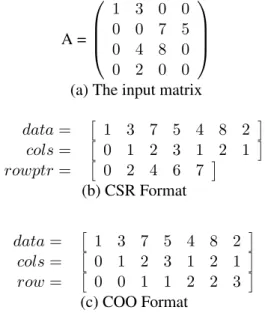
2.2.1 Compressed Sparse Row (CSR) Format

This is the popular storage format. This format stores only required elements and does not make any assumptions about sparsity pattern of the matrix. Let A be a sparse matrix with dimensionsM ×N and has nnz non-zeros. In this format we use three arrays say data, rowP tr, colP tr to store the matrix. The dataarray contains only nonzero elements of matrix. ThecolP tr stores column indices corresponding to the non-zeros in dataarray. In therowP tr we store starting and ending indices of each row indataarray. rowP tr[i],rowP tr[i+ 1]indicates the starting and ending indices ofithrow ofAindata,colP trarrays. The sizes ofrowP tr,colP tr,dataarem+ 1,nnz,nnzrespectively. An example of CSR format is given in 2.1(b).

2.2.2 Coordinate (COO) Format

This is also a popular store format. Let A be a sparse matrix with dimensions M ×N and has nnz non-zeros. Similar to CSR format, it also uses three arrays to store matrix. These three arrays aredata, rowindex, colindex. In similar to CSR format, dataarray stores only non zeros values of matrix A. rowindex, colindexstores row value, column value corresponding to non-zeros in data array respectively. So the three arrays are each of sizennzrespectively. An example of COO format is given in 2.1(c).

2.3

Sparse Matrix - Matrix Multiplication

Multiplication of two sparse matrices is also known as spgemm. It has applications in various domains such as graph algorithms [4, 5, 6], climate modeling, molecular dynamics, CFD solvers, and the like [7, 8, 9]. Multiplication of a sparse matrix with a dense matrix is known ascsrmm. It is an important kernel in linear algebra. It is used in iterative algorithms such as Lanczos method [28] and the Conjugate gradient method [28]. Implentation of spgemm is challenging because of sparsity nature of matrices, it poses severe load balancing problem among threads. As the prediction of output size is

(22)

A =     1 3 0 0 0 0 7 5 0 4 8 0 0 2 0 0    

(a) The input matrix

data= 1 3 7 5 4 8 2 cols= 0 1 2 3 1 2 1 rowptr= 0 2 4 6 7 (b) CSR Format data= 1 3 7 5 4 8 2 cols= 0 1 2 3 1 2 1 row= 0 0 1 1 2 2 3 (c) COO Format

Figure 2.1Different sparse matrix representations for an example matrix

difficult, it is also difficult to manage output memory. Because of SIMD nature execution of GPU, any divergence in execution path of warp also causes performance degradation.

2.3.1 Previous Work

Matrix matrix multiplication is a important problem in computer science. Because of its importance it has given a lot of attention in high performance. Efficient solutions for dense matrices are given on different architectures such as GPU [15], FPGA [17].

The first important work on spgemm was done by Gustavson et al. [19]. They developed a al-gorithm for spgemm and presentedspgemmin Row-Row formulation using CSR format. Now this algorithm is used in softwares such as [20] and CSparse [21]. Yuster el al. [26] considered spgemm

over a ring. They presented algorithms which use fast dense matrix multiplication algorithms. In [22] Park et al. gave a efficient data structure to store a class of sparse matrices in which non-zeros appear adjacently. By using this new data structure they presented a algorithm for fast sparse matrix multipli-cation.

Buluc et al. [23] extensively worked on spgemm. They explored scalable parallel algorithms for

spgemm on distributed memory systems. They have given data structures for hyper-sparse matrices. Also, they proposed 2D algorithms forspgemm and analyzed the scalability of 1D and 2D algorithms for parallel spgemm on distributed systems. They showed that existing 1D algorithms do not scale compared to 2D algorithms. Siegel et al. [24] developed a run-time framework forspgemmon hetero-geneous clusters. They introduced a task based programming model in which multiplication of block of

(23)

matrices represents a task. They also provided a run time execution model to address load balancing on clusters which consists of CPUs and GPUs. Sulatycke et al. [25] explored Row-Row, and Column-Row formulations of matrix multiplications and also presented cache optimized algorithms on sequential ma-chines forspgemm. The 2D matrix multiplication algorithms given in [18] are applicable for distributed systems not suitable for standalone systems.

As the programming model and architecture of GPU is different from distributed systems, the opti-mizations and algorithms proposed for distributed systems doesn’t suit to GPUs. To best of my knowl-edge no one has proposed any heterogeneous algorithm using CPU and a GPU forspgemm,csrmm. So we gave hybrid load balancing algorithms forspgemm,csrmm in next chapters.

2.4

Sparse Matrix Vector Multiplication

Multiplying a sparse matrix with a vector, usually denotedspmv, is one of the important problem in parallel computing with several applications to solve systems of linear equations using iterative methods like the conjugate gradient method, GMRES, iterative methods for finding eigenvalues and eigenvectors of sparse matrices, and the like [39]. These methods in turn find applications in many areas of Computer Science such as information extraction, image processing, and the like. The importance ofspmv can be judged by the fact that most multi-core architectures support an optimized library routine forspmv

[51, 42].

spmv computation offers a lot of data parallelism that can be exploited in a heterogeneous setting too. However, designing a heterogeneous algorithm for spmv requires one to address several chal-lenges. The amount of computation required with respect to a row of a matrix depends on the number of non-zeros in that row. In a general unstructured sparse matrix, the number of non-zeros per row can vary significantly across rows. Thus, it is difficult to apriori apportion the right amount of work, i.e the number of rows in this case, to the individual devices in a heterogeneous platform. An additional difficulty with respect tospmv arises from its typical usage, illustrated in Algorithm 1. In Algorithm 1, the function Modify can make suitable modifications to its input as dictated by the application. The

spmv kernel is often used in iterative methods and successive iterations use the vector generated in the previous iteration. If the vectorY is computed in pieces at both the CPU and the GPU, assuming that the function Modify can still be executed on both devices independently, the next iteration at the CPU requires the portion of theY vector computed at the GPU, and vice-versa. Hence, heterogeneous algo-rithms forspmv have to take into account the time required to transfer the partial vector from the CPU to the GPU and vice-versa at the end of every iteration. This places a hard synchronization requirement across the devices.

(24)

Algorithm 1A typical usage ofspmv.

Input:A sparse matrixA, a vectorX;

whilenot donedo

ComputeY :=A×X; Modify(Y);

X :=Y;

end while

2.4.1 Previous Work

Due to the fundamental nature of thespmv operation, there has been lot of studies done on im-plementingspmv efficiently on various architectures like multi-core CPU [63], GPU’s [40, 30, 32], FPGAs [36, 58] and vector architectures [34, 35]. Much of the above-cited work has focused on obtain-ing performance improvements of thespmv kernel by designing suitable data structures and identifying low level code optimizations.

In [64] Vuduc extensively studied optimizations onspmv and auto tuningspmv kernel for sequen-tial machines. In [63] Williams et al. studiedspmv on AMD dual core, Intel quad-core, STI Cell and Sun Niagara2. They presented optimization strategies for those multi-core environments. They have given low-level code optimizations and data structure optimizations that largely address single-core performance and parallelization optimizations to improve the multi-core performance.

Bell and Garland [33] proposed the CSR and the ELL matrix representation formats to store the sparse matrix on a GPU. Also, they proposedspmv kernels for different sparse matrix formats. Choi et al. [37] proposed a blocked ELLPACK data structure to store sparse matrix inspmv.

Monakov et al. [49] implement blockedspmv on GPU. In [50], Monakov et al. also proposed a sparse matrix data structure called Sliced ELLPACK, in which a slice of the matrix is a set of adjacent rows that are stored in ELL format. The size of each slice can be different. Each slice is assigned to a block of threads in CUDA. Load balancing of threads is achieved by assigning multiple threads to a row if required.

Another direction that is pursued recently is to consider special cases of sparse matrices and optimize the performance ofspmv for those special cases. Yang et al. [66] proposed optimizations for power law graphs. Their work improves the cache hit ratio of the texture cache of the GPU leading to increasing in the performance ofspmv.

Heterogeneous algorithms for spmv are not reported so far to the best of our knowledge. Such algorithms have been designed for related computations such as multiplying two sparse matrices [48], dense linear algebra computations [60], and the like.

Matching workload to a computational device based on the characteristics of the workload is an emerging line of research. In [41], Gharaibeh et al. consider three graph algorithms and suggest that for large, sparse graphs, it is advisable to process vertices of low degree on the GPU and vertices of high degree on the CPU. The authors of [41] also show that such a choice can help improve the hit ratio of

(25)

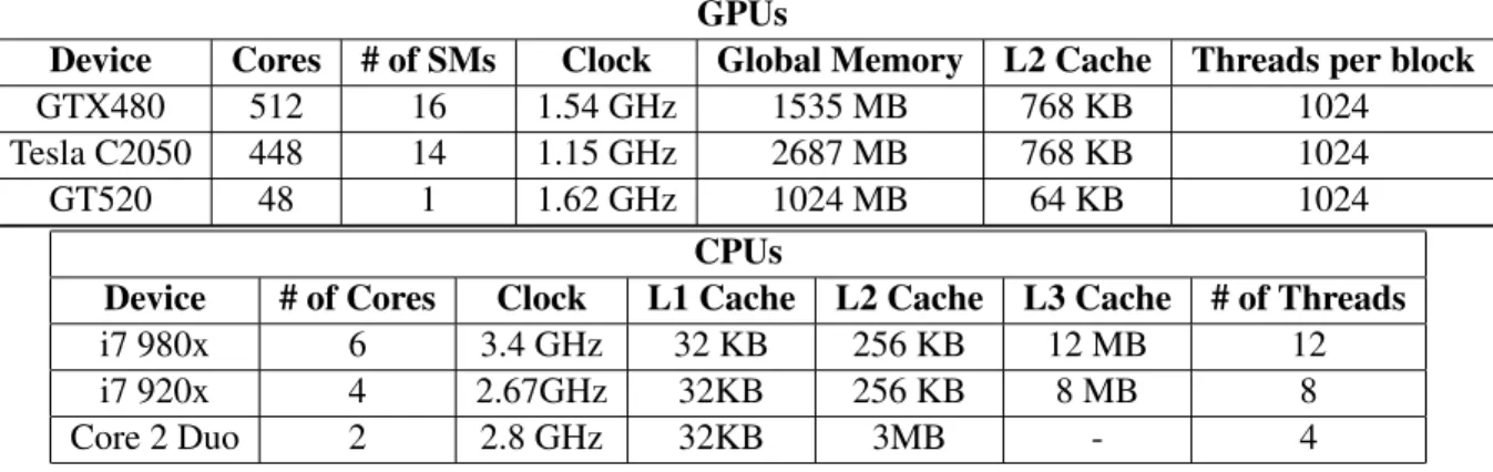
GPUs

Device Cores # of SMs Clock Global Memory L2 Cache Threads per block

GTX480 512 16 1.54 GHz 1535 MB 768 KB 1024

Tesla C2050 448 14 1.15 GHz 2687 MB 768 KB 1024

GT520 48 1 1.62 GHz 1024 MB 64 KB 1024

CPUs

Device # of Cores Clock L1 Cache L2 Cache L3 Cache # of Threads

i7 980x 6 3.4 GHz 32 KB 256 KB 12 MB 12

i7 920x 4 2.67GHz 32KB 256 KB 8 MB 8

Core 2 Duo 2 2.8 GHz 32KB 3MB - 4

Figure 2.2The specifications for the different GPUs and CPUs used in our experiments.

the last level cache on current multi-core architectures. In Chapter 3, we show similar effects can be seen for sparse matrix computations also.

2.5

Platforms

We experiment our algorithms on various platforms. Table 2.2 shows brief view about the CPUs and GPUs we used in our experiments. We use three heterogeneous platforms to evaluate our algorithms. The details of these heterogeneous platforms given below.

2.5.1 The Hetero-I

The Hetero-I heterogeneous platform we used is a coupling of the two devices, the Intel i7 980x CPU and the Nvidia GTX 480 GPU. The CPU and the GPU are connected via a PCI Express version 2.0 link which supports a data transfer bandwidth of 8 GB/s between the CPU and the GPU.

2.5.2 The Hetero-II

The Hetero-II platform consists of two devices, the Intel i7 920 CPU and the Tesla C2050 GPU. The CPU and the GPU are connected via a PCI Express version 2.0 link which supports a data transfer bandwidth of 8 GB/s between the CPU and the GPU.

2.5.3 The Hetero-III

The Hetero-III platform consists of two devices, the Intel core 2 duo CPU and the GT520 GPU. The CPU and the GPU are connected via a PCI Express version 2.0 link which supports a data transfer bandwidth of 8 GB/s between the CPU and the GPU.

(26)

2.6

Datasets

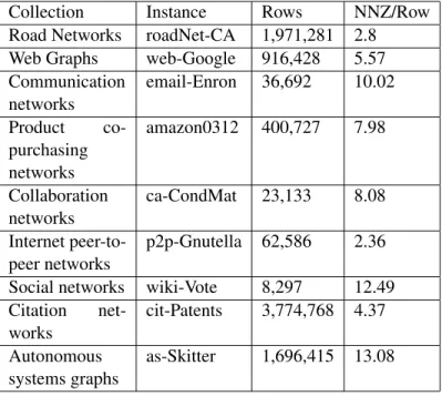
In our experiments we use datasets proposed by Williams et.al [33] which are shown in Figure 2.3. It contains 14 matrices which are from various fields such as circuits simulation, linear programming, finite element method based modeling etc. It contains matrices with different sparsity nature. Some of matrices have few non zero elements per row and some are highly unstructured in natured like LP and Webbase. We also use another set of sparse matrices, collected from SNAP sparse matrix collection [2] which are shown in Figure 2.4.

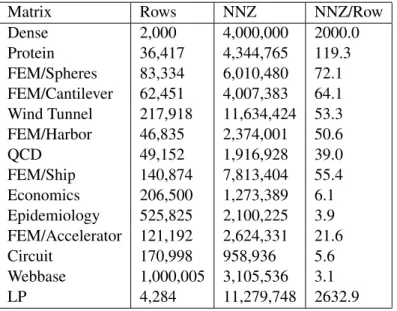
Matrix Rows NNZ NNZ/Row

Dense 2,000 4,000,000 2000.0 Protein 36,417 4,344,765 119.3 FEM/Spheres 83,334 6,010,480 72.1 FEM/Cantilever 62,451 4,007,383 64.1 Wind Tunnel 217,918 11,634,424 53.3 FEM/Harbor 46,835 2,374,001 50.6 QCD 49,152 1,916,928 39.0 FEM/Ship 140,874 7,813,404 55.4 Economics 206,500 1,273,389 6.1 Epidemiology 525,825 2,100,225 3.9 FEM/Accelerator 121,192 2,624,331 21.6 Circuit 170,998 958,936 5.6 Webbase 1,000,005 3,105,536 3.1 LP 4,284 11,279,748 2632.9

Figure 2.3List of sparse matrices. Number of columns and rows are equal for all the matrices except for the matrix LP, where the number of columns is equal to1,092,610.

(27)

Collection Instance Rows NNZ/Row Road Networks roadNet-CA 1,971,281 2.8 Web Graphs web-Google 916,428 5.57 Communication networks email-Enron 36,692 10.02 Product co-purchasing networks amazon0312 400,727 7.98 Collaboration networks ca-CondMat 23,133 8.08 Internet peer-to-peer networks p2p-Gnutella 62,586 2.36 Social networks wiki-Vote 8,297 12.49 Citation net-works cit-Patents 3,774,768 4.37 Autonomous systems graphs as-Skitter 1,696,415 13.08

(28)

Chapter 3

Static Load Balancing Algorithms For Sparse Matrix Kernels

This chapter gives a brief explanation about how we used static load balancing in our heterogeneous algorithms for sparse matrix operations along with the results.

3.1

Sparse Matrix - Sparse Matrix Multiplication(

spgemm

)

In this section we discuss about the algorithm, heuristics we use for work division among CPU, GPU and results.

3.1.1 Algorithm

LetA,Bbe two sparse matrices with sizesM×P,P×N respectively.C =A×Bis a matrix with sizeM×N. Recall from Chapter 2, We have four different formulations for matrix multiplication. We noticed that Row-Row formulation of matrix multiplication from [48] is performing better thancusp

libraryspgemm for sparse matrices. We also notice that the performance of spgemm on CPU is comparable to GPU [48]. So we extend the Row-Row algorithm to work as a heterogeneous algorithm. Our heterogeneous algorithm given in Algorithm 2, uses Row-Row formulation algorithm from [48] on GPU and Intel MKL libraryspgemm routine on CPU as it is efficient and standard. In Algorithm 2, the labels CPU (GPU), and GPU→ CPU, refer to steps executed on the CPU (resp. GPU), and data transfer from GPU to CPU. In our algorithm input matricesA,B are stored stored in CSR format and output matrixCis stored in COO format. We experiment on platform mentioned in Section 2.5.2.

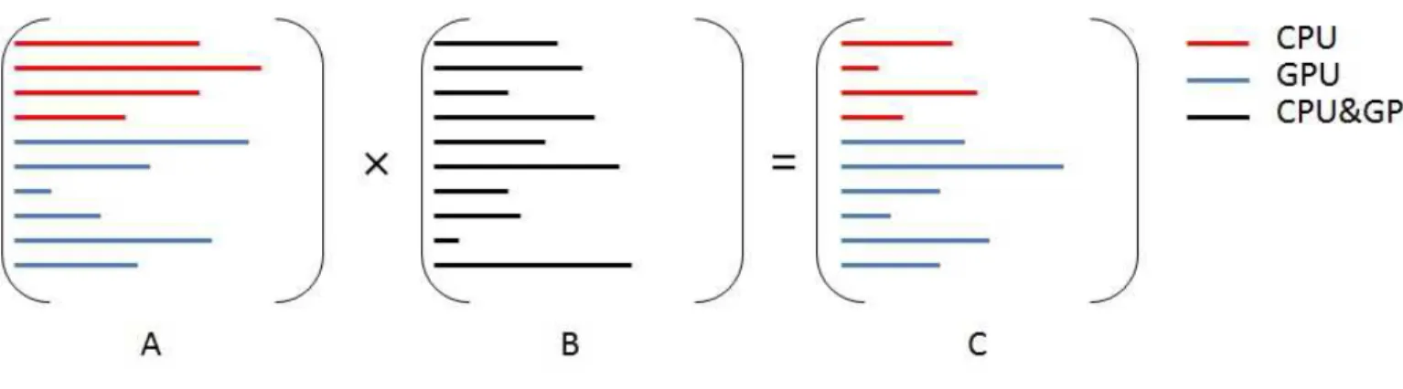
To divide the work among CPU and GPU we choose static load balancing strategy as follows. We choose a thresholdt%and assign the computation corresponding to first t%of the rows ofA (from top) to the CPU. The remaining computation is performed on the GPU. Let matrixACP U andAGP U be partial matrices which are processed on CPU and GPU respectively and matrix B is present on both CPU and GPU. LetCCP U and CGP U be the outputs computed by CPU and GPU respectively. After the computation, GPU transfers the output matrixCGP U onto the CPU. The final output is stored on CPU. The work division and computation is described in Figure 3.1. The challenge in designing

(29)

Figure 3.1spgemm using static load balancing. The red colored rows are processed on CPU and blue colored rows are processed on GPU.

Algorithm 2Heterogeneous Algorithm forspgemm

1: Identify a thresholdtat which to split the input matrix. Row number corresponding totisr. 2: A_CPU = A(1..r; :) and A_GPU = A(r + 1..M; :); //A_{CPU contains first} r rows of A, A_GPU

contains remaining rows.

3: CPU ::CCP U =CP U spgemm(A_CPU,B);//ComputeCCP U 4: CPU :: Wait for GPU to finish/*Synchronization*/

5: GPU ::CGP U =GP U spgemm(A_GPU,B);//ComputeCGP U 6: GPU→CPU : TransferCGP U to the CPU

(30)

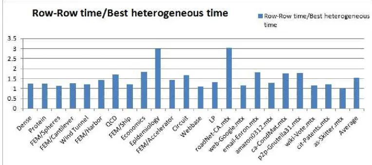
Figure 3.2 Performance comparison of heterogeneous method w.r.t Row-Row method on datasets shown in Figure 2.3, Figure 2.4 on Hetero-II given in Section 2.5.2.

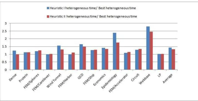
efficient hybrid algorithms then lies in finding the right threshold. A good value oftcan be obtained by exhaustive experimentation. We call the corresponding time asBest heterogeneous time. The result of the best heterogeneous times on platform given in Section 2.5.2 is shown in Figure 3.2. We notice that out heterogeneous algorithm has 1.5x speed up over GPU implementation on datasets given in Figure 2.3, Figure 2.4. However, exhaustive experimentation is not an ideal solution. Hence, we start with identifying heuristics to find a good value fort. We experiment with two different heuristics.

3.1.2 Heuristic I

In our first heuristic, we find the threshold based on the number of multiplications involved in an instance of spgemm when using the Row-Row formulation. For a sparse matrix A, let Ni(A) to denote the number of nonzero elements in theithrow ofA. LetIi(A)denote the indices of the nonzero elements in theithrow ofA. According to the Row-Row formulation, the number of multiplications for processing theithrow ofAinA×BisP

j∈Ii(A)|Nj(B)|. We observed that average GPU performance over CPU on the dataset from Figure 2.3 is around 3x[48]. So, we settto be 25% of the total number of multiplications. We findrwhich refers to the row number by whicht%of the multiplications occur. We then assign rows indexed 1 tor to be processed on the CPU and rowsr+ 1toM are processed on the GPU. The results of this heuristic are presented in Figure 3.3.

(31)

As can be observed, the best heterogeneous run time using the heterogeneous approach outperforms the hybrid run time obtained by using the proposed heuristic. Our heuristic considers only the average speedup to arrive at a value oftand the weakness of our heuristic can be attributed to that. To remedy this situation, we propose a better heuristic that takes the run time of Intel MKL and the GPU Row-Row formulation into account.

3.1.3 Heuristic II

In this heuristic, we delve a bit into each instance. We take the run time of the instance on CPU and also the GPU. Let these run times betcandtg. We take the thresholdtto be _t_ct_+tg_g%. As earlier, we find a value ofr so that the firstr rows account for t%of the multiplication operations. The results of using this heuristic are shown in the last column of Figure 3.3. As can be observed, this heuristic performs better than Heuristic I in general but still cannot meet the performance of the best possible heterogeneous approach. It clearly shows that finding best possible threshold value with heuristics is difficult.

The difficulty can be partly explained by the fact thatspgemm is a highly irregular computation. Moreover, it is difficult to estimate the number of rows that are required to make up a given percentage of the total number of operations. Knowing this, one can indeed estimate the size of the output matrix, which is one of the difficulties of thespgemm computation. Further, the highly unstructured sparsity nature of the matrices in the dataset from Figure 2.3 makes the tasks of estimating the threshold very difficult. It may therefore help if there is any prior knowledge on the nature of sparsity of the input matrices. We are able to design a analytical model to find best threshold value for band matrices which we explain in the next chapter.

3.2

Sparse Matrix - Dense Matrix Multiplication (

csrmm

)

3.2.1 Algorithm

LetAbe a sparse matrix in CSR format with size M ×P, B andC are dense matrices stored in row major format with sizesP ×N,M ×N andC = A×B. Similar tospgemm, the performance ofcsrmm on CPU and GPU are comparable. It is shown that GPU implementation ofcsrmm [48] is outperforming thecusparse library implementation ofcsrmm. So we devised a heterogeneous algorithm given in Algorithm 3, which uses GPU implementation ofcsrmm [48] on GPU and Intel MKL library [42]csrmm routine on CPU as it is efficient and standard. In Algorithm 3, the labels CPU (GPU), and CPU→GPU (GPU→CPU), refer to steps executed on the CPU (resp.GPU), and data transfer from CPU to GPU (resp.GPU to CPU).

In similar tospgemm, we choose a threshold t% and assign the computation corresponding to t% of the rows of A to the CPU. The remaining computation is performed on the GPU. Let matrixACP U and AGP U be partial matrices which are processed on CPU and GPU respectively and matrixB is present

(32)

Figure 3.3Performance comparison of two presented heuristics w.r.t the best heterogeneous timings on the dataset shown in Figure 2.3 on platform Hetero-II given in Section 2.5.2. X-axis represents instances in dataset and Y-axis represents performance w.r.t best heterogeneous time. The last instanceAverage shows the average value of the series.

Algorithm 3Heterogeneous Algorithm forcsrmm

1: Identify a thresholdtat which to split the input matrix. Row number corresponding totisr. 2: A_CPU = A(1..r; :) and A_GPU = A(r + 1..M; :); //A_{CPU contains first} r rows of A, A_GPU

contains remaining rows.

3: CPU ::CCP U =CP U csrmm(A_CPU,B);//ComputeCCP U 4: CPU→GPU : TransferCCP U to the GPU

5: CPU :: Wait for GPU to finish/*Synchronization*/

6: GPU ::CGP U =GP U csrmm(A_GPU,B);//ComputeCGP U 7: GPU→CPU : TransferCGP U to the CPU

(33)

Figure 3.4Performance comparison of heterogeneous algorithm w.r.t GPU algorithm forcsrmm[48] on dataset shown in Figure 2.3 on the Hetero-I given in Section 2.5.1.

on both CPU and GPU. LetCCP U andCGP U be the outputs computed by CPU and GPU respectively. Ascsrmm is a iterative algorithm, GPU transfers the output matrix CGP U onto the CPU and CPU transfers theCCP U onto the GPU. So that both CPU and GPU will have final output matrix.

3.2.2 Results

We experiment our algorithm on platform mentioned in 2.5.1 using dataset given in figure 2.3. We vary the threshold valuetfrom 0 to 100. Best value oft is obtained by exhaustive experimentation. Performance comparison of our heterogeneous algorithm and GPU algorithm[48] is shown in Figure 3.4. Our heterogeneous algorithm is up to 15% faster compared to GPU algorithm. It can be observed that some instances such as Economics, Epidemiology, Circuit, Webbase are not performing well with heterogeneous algorithm. Because the computation time less than the transfer time in those matrices.

3.3

Sparse Matrix Vector Multiplication(

spmv

)

In this section we give an example which shows that multiplying a sparse matrix with a vector can be done by reordering the rows of matrixAand the vectorXsuitably. We make use of such a reordering in our work division algorithms. Later we discuss about work divisions schemes along with results.

(34)

3.3.1 Reordering Rows ofAinspmv

The spmv computation is typically used in many iterative methods such as Lanczos iterations, Arnoldi iterations and the like [39]. These methods run thespmv kernel for around 300–1000 iter-ations. In each iteration the vector will be updated according to certain rules and the updated vector is used in next iteration. The rules in these method are generally scalar addition/multiplication of a vector and subtraction of vectors. All these operations will not be effected by rearrangement of input vector and input matrix. Hence, in some of our work division algorithms, we rely on the above fact. This is illustrated with an example below.

LetAbe anM×Mmatrix andXis initial vector with sizeM×1. LetA1be the matrix obtained after rearranging the rows ofAbased on increasing number of non-zeros per row. Let the vectorXbe also rearranged accordingly, and call the resulting vector asX1. LetA2 be the matrix obtained after rearranging the columns ofA1based on number of non-zeros per row ofA. LetR= [r1,r2,...,rM] be an array represents the row numbers ofAwhich are sorted in ascending order of number of non-zeros per row where1≤ri≤M and1≤i≤M. Notice thatX1[k]is equal toX[R[k]]. For a matrixA, let A(i; :), A(:;i)denote the ith row and theith column ofArespectively. NowA1(r[k]; :) = A(R[k]; :) andA2(:;k)= A1(:;R[k]). With this notation, we give an example below to show the reordering the rows and columns of a matrixAdoes not affect the output ofA×Xbeyond a corresponding reordering.

A=       1 2 1 −1 0 1 2 −2 0 1 0 1 1 0 2 1       X =       1 1 2 1       R=       3 2 4 1       A1 =       0 1 0 1 0 1 2 −2 1 0 2 1 1 2 1 −1       A2 =       0 1 1 0 2 1 −2 0 2 0 1 1 1 2 −1 1       , and X1 = h 2 1 1 1 iT

Without any reordering, we get thatA×X =

h

4 3 2 6

iT

, and pre-multiplying the resulting vector withAagain, we get the vectorh6 −5 9 14

iT

.

With a reordering of the rows and columns ofAand the elements ofX, the resulting vectors during the first two iterations are computed as follows. A2 ×X1 =

h

2 3 6 4

iT

and pre-multiplying this vector withA2yields the vector

h

9 −5 14 6

iT

.

We can see from the above example that the output produced in ith iteration by multiplying pre-processed initial matrix, and input vector in every iteration is identical to a rearrangement of output produced in ith iteration by multiplication actual matrix and actual vector. So it is sufficient if we rearrange the final output.

(35)

3.3.2 Work Division Schemes

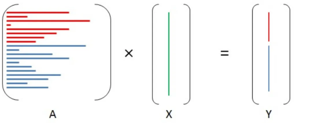
In this section we describe three work division schemes forspmv. LetAbe input matrix with size M×M andXbe a vector of sizeM×1. LetY =A×Xbe the result vector with sizeM×1. Note that the spmv workload possesses data parallelism and hence it is possible to divide the computation across devices also. However, there are two algorithmic challenges that one has to address.

Firstly, the computational methodology of the CPU and the GPU are vastly different. Hence, one has to understand how to match the right kind of work to each device. For instance, should rows with several non-zero elements be processed on the CPU or the GPU? Secondly, the volume of computation involved per row varies according to the number of non-zeros in that row. Hence, one has to identify the right amount of work division across the devices. It has to be noted however that one seeks simple yet effective solutions for both the above challenges.

In this section, we present three possible approaches for work division with respect tospmv. Later sections address the questions of matching the right work to the right device, and the quantum of work. All the three work division methods that we present in this section are based on the criteria that arriving at the work division is as simple as sorting the rows of the matrix on the number on non-zeros.

• Direct-Division : This scheme involves dividing the matrix A into two matrices A_{CPU and} A_{GPU. Let} r be a number between 1 tom. Then,A_{CPU consists of rows 1 to}r andA_GPU consists of rowsr+ 1tom. Choosingrcan be done empirically.

Figure 3.5Figure shows the Direct-Division scheme forspmv. The red colored rows ofAare processed on the CPU, and the other rows are processed on the GPU. The corresponding portion of the result vector in each iteration is also colored accordingly.

• Large-Rows-GPU :In this scheme, we first sort the rows ofAin increasing order of the number of non-zeros and rearrange the matrix, vector accordingly like we explained in Section 3.3.1. Then, we pick a numberr between 1 toM. We then define the two matricesA_{CPU and}A_GPU as earlier. The matrixA_{CPU consists of rows 1 to}rofA, andA_{GPU consists of rows}r+ 1to M.

(36)

Figure 3.6 Figure shows the Large-Rows-GPU scheme for spmv. The red colored rows of A are processed on the CPU, and the other rows are processed on the GPU. The corresponding portion of the result vector in each iteration is also colored accordingly.

• Small-Rows-GPU :In this scheme, as in the earlier scheme, we sort the rows ofAin descending order of the number of non-zeros per row and rearrange the matrix , vector accordingly like we explained in Section 3.3.1. Then, a numberr between 1 toM is chosen. The matrices A_CPU andA_{GPU are then defined as the matrix consisting of rows 1 to} r and rowsr+ 1 toM ofA respectively.

Figure 3.7 Figure shows the Small-Rows-GPU scheme for spmv. The red colored rows of A are processed on the CPU, and the other rows are processed on the GPU. The corresponding portion of the result vector in each iteration is also colored accordingly.

Figure 3.5, Figure 3.6 and Figure 3.7 illustrate the above work division schemes. All the above methods can use a common algorithmic model described below. The main algorithm we use is Algorithm 4 that creates two matrices A_{CPU and}A_{GPU. For a matrix} A ofM rows and positive integers1 ≤ a < b ≤M, we useA(a..b; :)to indicate the sub matrix obtained by taking rows numberedatobofA. In Algorithm 4, the labels CPU (GPU), and CPU→ GPU (GPU→ CPU), refer to steps executed on the CPU (resp. GPU), and data transfer from CPU to GPU (resp. GPU to CPU). On multi-core CPUs, the

(37)

spmv library routine from Intel MKL [42] is the best known reported implementation. Hence, we use this routine onA_{CPU. Let us call the output of this computation as}Y_{CPU. Similarly, on the GPU, we} make use of thespmv routine in thecusp library provided by Nvidia [51]. This is the best known reported implementation on GPUs for general sparse matrices. Let us call this output asY_{GPU. Now,} Steps 6 and 10 of Algorithm 4 call for transfer ofY_{CPU from the CPU to the GPU and the transfer of} Y_{GPU from the GPU to the CPU. This step is required so that the next iteration at the CPU and the GPU} has access to the entireBvector computed in this iteration.

Algorithm 4Heterogeneous Algorithm forspmv

1: Identify a row numberrat which to split the input matrix; 2: A_CPU=A(1..r; :)andA_GPU=A(r+ 1..m; :);

3: X_CPU0 =X_GPU0 =B; 4: fori= 0 toniterationsdo

5: CPU ::Y_CPU=CP U spmv(A_CPU, X_CPUi , Ci); 6: CPU→GPU :: TransferY_{CPU to the GPU.}

7: CPU :: Wait for GPU to finish/*Synchronization*/

8: AppendY_{CPU to}Y_{GPU to get}Cion GPU side; 9: GPU ::Y_GPU=GP U spmv(A_GPU, X_GPUi , Ci); 10: GPU→CPU : TransferY_{GPU to the CPU}

11: GPU :: Wait for CPU to finish/*Synchronization*/

12: GPU :: AppendY_{GPU to}Y_{CPU to get}Cion GPU side; 13: CPU::X_CPUi+1 =Ci;

14: CPU::X_GPUi+1 =Ci; 15: end for

3.3.3 Experimental Results

We evaluate our heterogeneous algorithms on the platform mentioned in Section 2.5.1 using two datasets. One is the standard dataset proposed by Williams et al. [63] shown in Table 2.3. This dataset has been the choice dataset for several recent works onspmv [50, 49, 48]. We also consider a dataset containing a sample of matrices from the University of Florida sparse matrix collection [38]. These matrices are shown in Table 2.4.

The results of the three work division schemes on the dataset from Table 2.3 and on the dataset from Table 2.4 are shown in Figure 3.8(a) and 3.8(b) respectively. The label “Pure GPU” in Figure 3.8 refers tospmv implementation fromcusp[51]. We show the relative speed-up of the three work division methods with respect tospmv implementation fromcusp[51]. It can be noted that all the three work division schemes generally outperform a pure GPU alone implementation. In some cases, we can notice an improvement of 45 % (e.g., matrix FEM/Harbor from Figure 3.8(a)), and an average improvement of 20 %.

(38)

0 0.5 1 1.5 2 2.5 Dense _Protein FEM/Spheres FEM/Cantilever WindTunnel FEM/Harbor QCD FEM/Ship _Economics Epidemiology FEM/Accelerator Circuit Webbase Average 1 1.1 1.2 1.3 1.4 1.5

Speedup over GPU

Max/Min Matrix Instance Pure GPU/Direct-Division Pure GPU/Small-Rows-GPU Pure GPU/Large-Rows-GPU Max/Min

(a) Dataset from Table 2.3

0 0.5 1 1.5 2 amazon0312 internet web-google dblp-2010 p2p-Gnutella31

ca-CondMat email-Enron cit-patents

as-Skitter wiki-vote Average 1 1.05 1.1 1.15 1.2 1.25 1.3 1.35 1.4

Speedup over GPU

Max/Min Matrix Instance Pure GPU/Direct-Division Pure GPU/Small-Rows-GPU Pure GPU/Large-Rows-GPU Max/Min

(b) Dataset from Table 2.4

Figure 3.8Performance comparison of execution times of the three work division methods for sparse matrices from two different datasets on platform given in 2.5.1. The line anchored to the second Y-axis, labeled Max/Min, measures the ratio of the best speed-up to the least speed-up among the three work

(39)

It is however interesting to note that no single scheme has a clear advantage across the matrices considered. Some of this can be explained by the following reasoning. The matrices considered in the dataset have widely varying nature of sparsity. In some cases, for example the Epidemiology matrix has most of the rows with 4 non-zero elements. In this case, a pure GPU implementation can outperform a heterogeneous implementation because of identical and small workload across GPU threads. In a heterogeneous implementation on this matrix, the time taken to transfer the result vector dominates the compute time required by either device. That is indeed the case in other instances also such as Internet, p2p-Gnutella31, wiki-vote.

Some matrices such as Protein, FEM/Spheres, FEM/Harbor from Table 2.3 exhibit a strong degree of locality with respect to the column indices of the non-zero elements. This can be observed also from the row-column plots of the matrices1. This means that while all the three work division methods presented earlier outperform a non-heterogeneous implementation, there is very little difference between the three heterogeneous algorithms. This phenomenon is illustrated in Figure 3.8 via the Max/Min line anchored to the second Y-axis. For the above matrices, among the three work division methods, the ratio of the best speed-up achieved to that of the least speed-up achieved with respect to a GPU alone implementation is under 10%.

Figure 3.9Figure showing the timeline of two iterations ofspmv on the matrix FEM/Cantilever from Table 2.3. The labels CPU and GPU indicate computations on the CPU and the GPU respectively. The labels CPU→GPU and GPU→CPU indicate transfer of the partial result vector from the CPU to the GPU and vice-versa.

For another set of matrices such as Wind Tunnel, Economics, FEM/Accelerator, and FEM/Cantilever, the number of non-zeros in each row is near-uniform, and also is moderate in number. This means that there is not much difference in how the three methods partition the workload. Therefore, we see very little difference in the speed-up achieved by the three methods. It should be noted however that all the three methods outperform a non-heterogeneous implementation on these matrices.

1

(40)

However, for matrices such as Circuit and Webbase from Table 2.3, and matrices such as ama-zon0312, internet, web-google, dblp-2010, p2p-Gnutella31, ca-CondMat from Table 2.4, the Small-Rows-GPU method outperforms the other methods considerably. The reason for this is explained in the following Section 3.3.4.

To study the efficiency of our implementation in utilizing the CPU and the GPU, we show the work done by the CPU and the GPU on the FEM/Cantilever matrix from Table 2.3 on a timescale in Figure 3.9. Figure 3.9 also shows the time taken to transfer the result vector in each iteration. It can be noticed from Figure 3.9 that our implementation is able to match the computation and transfer time required by the CPU and the GPU very closely. This also indicates that our implementation suffers from a very small idle time either for the CPU or the GPU.

It is possible that we can further reduce the idle time by using a standard double buffering technique at both the CPU and the GPU to overlap the computation with data transfer. However, this means that the calls to thespmv routine in the MKL library and thecusp library have to be issued multiple time on portions ofA_{CPU and}A_{GPU respectively. Also, multiple calls have to be issued for initiating the} transfer of partialY_{CPU to the GPU and the partial}Y_{GPU to the CPU. These additional calls result in} an overhead that outweigh the advantages of double buffering.

3.3.4 Scale-free Matrices

A matrix is said to exhibit scale-free nature if the matrix has several rows with very few non-zero elements per row, and a very few rows with a large number of non-zero elements. Such matrices arise in several practical settings including transportation networks, web search, Internet algorithmics, and the like as the matrices underlying such computations tend to be scale-free. It is observed that some matrices from Table 2.3, Table 2.4 have a large majority of the rows with a small number non-zero elements per row, and there are very few rows with a large number non-zero elements per row. It is to be noted that the threshold of whether a row has a small number of non-zeros varies with the matrix, from order of hundred for the webbase matrix to less than 50 for the Circuit matrix. In this section, we show that the Small-Rows-GPU scheme of work division suits for scale-free matrices along with evidence for the same.

The algorithm we use is described in Algorithm 4. We identify the matricesA_{CPU and}A_{GPU using} an empirical exhaustive search to identify the best possible division amongst the CPU and the GPU. Figure 3.10 shows the result of applying this division scheme on a collection of scale-free matrices taken from the dataset of Table 2.3 and Table 2.4. As can be noticed, the Small-Rows-GPU method outperforms a GPU alone implementation and also the other three methods except in cases where the transfer time dominates the compute time as in matrices such as Internet, and p2p-Gnutella31. In the other cases, the average improvement is noted to be 20 %.

We offer two explanations for this behavior. Firstly, we investigate the cache-hit ratio of the last level cache on the CPU used in our experiments. In Figure 3.11, we compare the cache hit ratio of two schemes, Small-Rows-GPU and Large-Rows-GPU, on four different scale-free matrices used in

(41)

our experiments. As can be seen from Figure 3.11, when large rows are processed on the CPU, indeed there is an improvement in the cache-hit ratio. In some instances, e.g., the matrix webbase, the cache hit ratio for the Small-Rows-GPU method is much better than for the Large-Rows-GPU method. This augurs well for the computation.

On the other hand, small rows happen to be a good fit for the GPU. In the GPU workload consisting of rows with small number of non-zero elements, it is likely that threads in a warp have near-identical work. So, there is lesser chances of load imbalance across threads in a warp leading to better performance on a GPU. One can also see increased occupancy also as each thread brings in only few elements into the shared memory and registers.

0 0.5 1 1.5 2

Circuit

Webbase

amazon0312

internet

web-google

dblp-2010

p2p-Gnutella31

ca-CondMat

Average

Speedup over GPU

Matrix Instance Pure GPU/Direct-Division Pure GPU/Small-Rows-GPU Pure GPU/Large-Rows-GPU

Figure 3.10Applying the Small-Rows-GPU method to scale-free matrices from the datasets of Table 2.3 and 2.4 on platform given in 2.5.1. The last item on the X-axis refers to the average of the series.

For the above reasons, the Small-Rows-GPU work division scheme suits for scale free matrices. One drawback however is that we need to do exhaustive search to find best work division. The next chapter answers this question using a workqueue framework.

(42)

88 90 92 94 96 98 100 0 20 40 60 80 100

Cache hit rate

%nonzeros Small-Rows-GPU Large-Rows-GPU

(a) Matrix : Circuit

10 20 30 40 50 60 70 80 90 100 0 20 40 60 80 100

Cache hit rate

%nonzeros Small-Rows-GPU Large-Rows-GPU (b) Matrix : Webbase 80 85 90 95 100 0 20 40 60 80 100

Cache hit rate

%nonzeros Small-Rows-GPU Large-Rows-GPU (c) Matrix : Web-Google 80 85 90 95 100 0 20 40 60 80 100

Cache hit rate

%nonzeros Small-Rows-GPU Large-Rows-GPU

(d) Matrix : DBLP-2010

Figure 3.11Cache hit ratio on the CPU last level cache for four different scale-free matrices. The X-axis indicates the percentage of the total number of non-zeros that were assigned to the CPU.

(43)

Chapter 4

Dynamic Load Balancing Algorithms For Sparse Matrix Kernels

The challenging problem in any heterogeneous algorithm is to divide the work among heterogeneous devices. We have to do an exhaustive search to find the best possible work division, which takes a lot of time. Also, static partitioning of irrespective of instance lead to load imbalances. So we devised a work queue frame work to address the load balancing problem. In this chapter we give a brief explanation of our work queue frame work. Also we discuss about how we used this frame work to achieve dynamic load balancing in sparse matrix operations along with results.

4.1

Work Queue Model

4.1.1 Framework

In this section, we observe that workloads such as sparse matrix operations possess a few character-istics that make them amenable for dynamic load balancing even in heterogeneous environments. These characteristics are listed below.

• Independent work units: The computation can be broken down into independent subproblems calledwork units. It is not necessary that the work units have identical computational requirement.

• Easily describable work units: These workloads have easy and succinct to describe independent subproblems. For instance, a work unit could correspond to processing a contiguous set of ele-ments, say rows in a matrix.

• Minimal or no post-processing: The solution to the entire problem be a (near)-immediate con-sequence of the solutions to the independent work units. There should be little post-processing involved.

Dynamic load balancing of the above category of workloads can be achieved by having multiple threads of the CPU and the GPU share a queue that contains several work units. The individual threads can access the work queue to fetch the next work unit for which computation is still pending. The

(44)

Figure 4.1Work Queue model

CPU threads and the GPU access the work queue from either end so that there is no need to, in most cases, synchronize accesses to the work queue by the CPU and the GPU. However, CPU threads have to access the queue in a concurrent fashion. Given the low number of CPU threads that we use, we employ a simple locking mechanism on the CPU front variable. We also perform the following further optimizations for improved performance.

• Minimal Synchronization: To minimize the synchronization requirement when accessing the queue, we make the queue double-ended. The CPU and the GPU dequeue work units from either ends. The only synchronization required between the CPU and the GPU is for dequeuing the last work unit from the queue. Having a double ended queue also ensures that it is easy to maintain the state of the queue correctly at all times. In practice, we also notice that the synchronization requirement is also most non-existent. In sparse matrix operations, they have work units that are independent. So this optimization is possible.

• Reducing the Overhead of Queue operations: Secondly, the overhead of queue operations is kept at a minimum by maintaining logically, and not physically. So, we do not actually fill the queue with work units before the start of the computation. Assuming a total ofnwork units initially, the frontpointer on the CPU side is set at work unit 1, and the front pointer on the GPU side is set work unit n. The frontpointer at each end can completely describe the progress of the computation. The computation is said to finish when thefrontpointer on the GPU side meets, or crosses, thefrontpointer on the CPU side. Since in the sparse matrix operations, the computation has work units are succinctly describable, this optimization is possible.

• Other Program Optimizations: To keep this overhead of GPU kernel launches low, we launch the GPU kernel only once irrespective of the number of work units that the GPU works. The GPU kernel interacts with the host to fetch multiple work units without exiting execution on the device.

(45)

4.2

Sparse Matrix - Matrix Multiplication

Multiplying a sparse matrix with another sparse/dense matrix is an important workload in parallel computing. These operations, calledspgemm and csrmmrespectively, have applications to several problems from various domains. For instance,spgemm has applications to problems from engineering such as graph algorithms [4], numerical applications including climate modeling, molecular dynamics, CFD solvers, and so on. csrmmis widely used in Krylov subspace methods such as Lancozs method a