Scalable Systems for Large Scale Dynamic Connected Data Processing

(1)

Title

Scalable Systems for Large Scale Dynamic Connected Data Processing Permalink

https://escholarship.org/uc/item/9029r41v Author

Padmanabha Iyer, Anand Publication Date 2019

Peer reviewed|Thesis/dissertation

eScholarship.org Powered by the California Digital Library

(2)

by

Anand Padmanabha Iyer

A dissertation submitted in partial satisfaction of the requirements for the degree of

Doctor of Philosophy in Computer Science in the Graduate Division of the

University of California, Berkeley

Committee in charge: Professor Ion Stoica, Chair

Professor Scott Shenker Professor Michael J. Franklin

Professor Joshua Bloom

(3)

by

(4)

Abstract

Scalable Systems for Large Scale Dynamic Connected Data Processing by

Anand Padmanabha Iyer

Doctor of Philosophy in Computer Science University of California, Berkeley

Professor Ion Stoica, Chair

As the proliferation of sensors rapidly make the Internet-of-Things (IoT) a reality, the devices and sensors in this ecosystem—such as smartphones, video cameras, home automation systems, and autonomous vehicles—constantly map out the real-world producing unprecedented amounts of dynamic, connected datathat captures complex and diverse relations. Unfortunately, existing big data processing and machine learning frameworks are ill-suited for analyzing such dynamic connected data and face several challenges when employed for this purpose.

This dissertation focuses on the design and implementation of scalable systems for dynamic connected data processing. We discuss simple abstractions that make it easy to operate on such data, efficient data structures for state management, and computation models that reduce redundant work. We also describe how bridging theory and practice with algorithms and techniques that leverage approximation and streaming theory can significantly speed up connected data computations. Leveraging these, the systems described in this dissertation achieve more than an order of magnitude improvement over the state-of-the-art.

(5)

(6)

List of Figures

1.1 Alex, a network administrator, diagnoses issues using data collected in the

network. . . 2 1.2 Taylor, a financial analyst, uses transaction data to train a model to detect

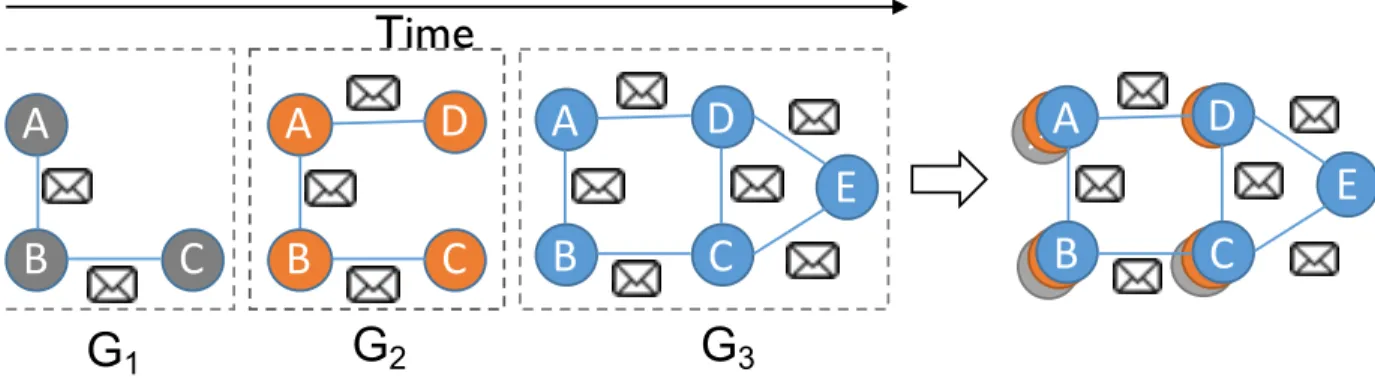
money laundering. . . 3 1.3 Representing connected data as property graphs. . . 6 3.1 A timelapse of graphGconsisting of three snapshots. For temporal analytics,

instead of applying graph-parallel operations independently on each snapshot (left), timelapse enables them to be applied to all snapshots in parallel (right). 20 3.2 1 Connected components by label propagation on snapshotG₁produces R₁.

2 Vertex Aand edgeA−Bis deleted inG₂. Using the last result to bootstrap

computation results in incorrect answer R2. 3 A strawman approach of

storing all messages during the initial execution and replaying it produces correct results, but needs to store large amounts of state. . . 21 3.3 Two examples that depict how ICE works. Dotted circles indicate vertices

that recompute, and double circles indicate vertices that need to be present in the subgraph to compute the correct answer, but do not recompute state themselves. 1 Iterations of initial execution is stored in the timelapse. 2 ICE

bootstraps computation on a new snapshot, by finding the subgraph consisting of affected vertices and their dependencies (neighbors). In the second example,

Cis affected by the deletion of A−C. To recompute state it needs D(yields subgraph C−D). 3 At every iteration, after execution of the computation

on the subgraph, ICE copies state for entities that did not recompute. Then finds the new subgraph to compute by comparing the previous subgraph to the timelapse snapshot. In the second example, though C recomputes the same value as in previous iteration, its state is different from the snapshot in timelapse and hence needs to be propagated. 4 ICE terminates when the

subgraph converges and no entity in the graph needs the state copied from stored snapshots in the timelapse. . . 23

(11)

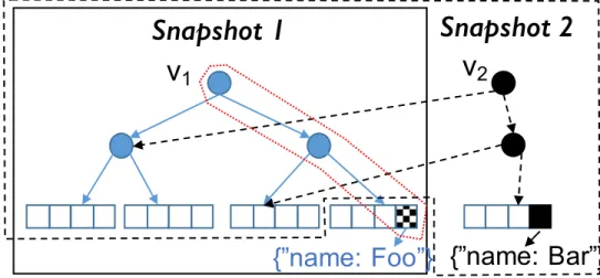
edges on each of the partitions. Here, a vertex pART stores properties in its leaves. Vertex id traverses the tree to the leaf storing its property. Changes generate new versions. . . 27 3.5 DGSI has fine-grained control over leaves (where data is stored). Here DGSI

has 1000s of snapshots. All snapshots exceptS is on disk, their parents just

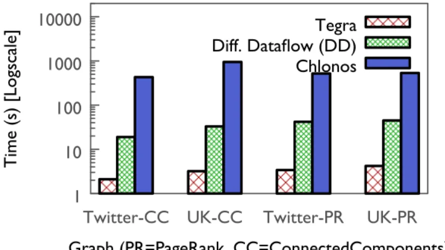
hold pointers to the file. Parents are also dynamically written to disk if all of their children are on disk. Datastructure uses adaptive leaf sizes for efficiency. 29 3.6 Snapshot retrieval latency in DD incurs cost and degrades with time. . . 33 3.7 Differential dataflow generates state at every operator, while Te g r a’s state is

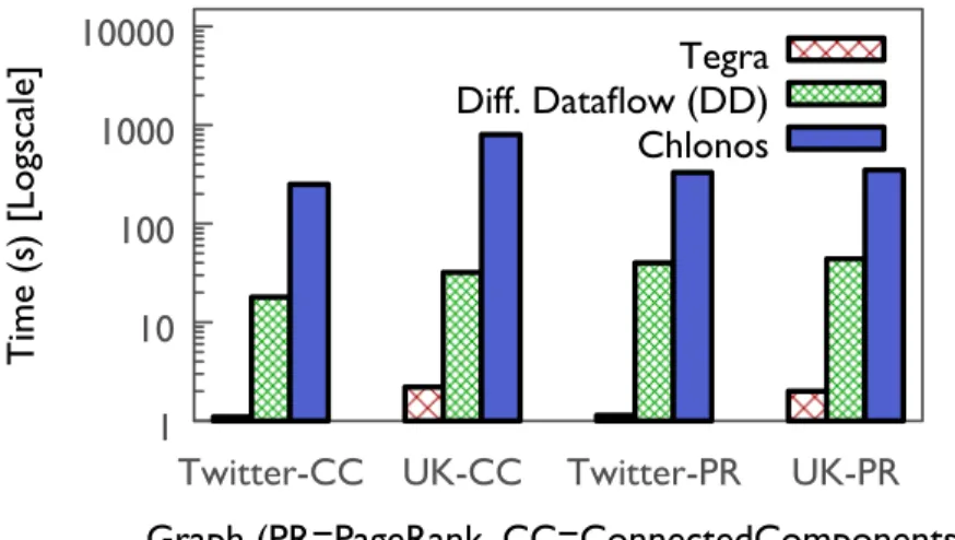
proportional to the number of vertices. . . 33 3.8 On ad-hoc queries on snapshots, Te g r a is able to significantly outperform

due to state reuse. . . 34 3.9 Te g r a’s performance is superior on ad-hoc window operations even with

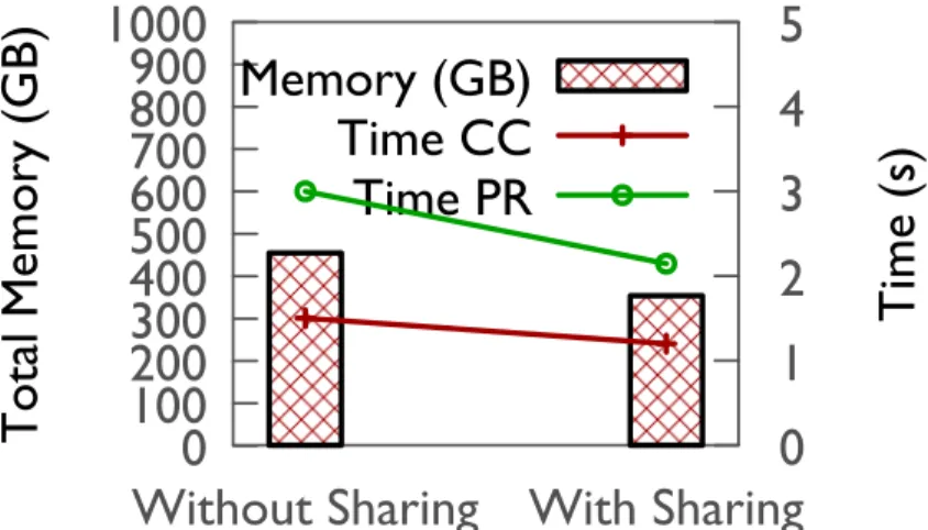
materialization of results. . . 35 3.10 Timelapse can be used to optimize graph-parallel stage. . . 37 3.11 Sharing state across queries results in reduction in memory usage and also

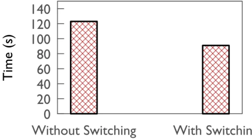
improvement in performance. . . 37 3.12 Incremental computations are not always useful. Te g r a can switch to full

re-execution when this is the case. . . 38 3.13 Monotonicity of updates (additions only) can be leveraged to speed up

com-putations by starting from the last answer. . . 39 3.14 DD significantly outperforms Te g r a for purely streaming analysis. . . 39 4.1 Simply extending approximate processing techniques to graph pattern mining

does not work. . . 46 4.2 Triangle count by neighborhood sampling . . . 49 4.3 ASAP architecture . . . 50 4.4 Two ways to sample four cliques. (a) Sample two adjacent edges (0,1) and

(0,3), sample another adjacent edge(1,2), and wait for the other three edges. (b) Sample two disjoint edges(0,1)and (2,3), and wait for the other four edges. 52 4.5 Example approximate pattern mining programs written using ASAP API . . . 58 4.6 Runtime with graph partition. . . 59 4.7 The actual relations between number of estimators and run-time or error rate. 62 4.8 ASAP is able to gain up to77×improvement in performance against Arabesque.

The gains increase with larger graphs and more complex patterns. Y-axis is in log-scale. . . 66 4.9 Runtime vs. number of estimators for Twitter, Friendster, and UK graphs. The

black solid lines are ASAP’s fitted lines. . . 69 4.10 Error vs. number of estimators for Twitter, Friendster, and UK graphs. . . 71 4.11 CDF of100runs with3% error target. . . 72

(12)

4.12 The errors from two cluster scenarios with different number of nodes.

Config-1:strong-scaling to fix the total number of estimators as 2M × 128; Config-2:

weak-scaling to fix the number of estimators per executor as2M. . . 72

4.13 Two representative (from21) patterns in5-Motif. . . 73 5.1 Sampling randomly leads to undesirable effects. Here, execution time (speedup)

increases (reduces) with smaller samples. . . 78 5.2 G A P System Architecture. . . 80 5.3 In triangle counting, we see similar trends in performance in graphs with

similar characteristics (e.g., AstroPh & Facebook). . . 83 5.4 Error due to sparsification. Like the speedup, we see similarity in the error

profile of graphs with similar characteristics. . . 83 5.5 Larger graph (uk-2007-05[33, 31] with3.7B edges) sees better speedup due to

the distributed nature of the execution. . . 84 6.1 Mo n a r c h system architecture. Each data center (DC) contains part of the

graph. Communication between DCs happen through border vertices (shaded vertex in the picture), who exchange and synchronize state as described in §6.3. 90 6.2 In incremental GAS model, each iteration marks and activates the

neighbor-hood it influences. In this example, border vertex A is updated. It marks and activates B in the first iteration, B marks and activates C in the second iteration and C marks and activates D in the third. By leveraging the characteristics of the algorithm being executed, we avoid marking E and F although they are in the immediate neighborhood of C and B. . . 93 6.3 Our proposal is able to complete the execution of connected components when

GraphX is unable to complete. This is because it tries to transfer too much data across WAN. . . 94 7.1 LTE network architecture . . . 98 7.2 Simply applying ML for RAN performance diagnosis results in a fundamental

trade-off between latency and accuracy. . . 101 7.3 Ce l lSc o p e System Architecture. . . 104 7.4 Ce l lSc o p e achieves high accuracy while reducing the data collection latency.115 7.5 Other domains suffer from latency-accuracy trade-off. Here, we see the

prob-lem in the domain of energy debugging for mobile devices. Grouping by phone model or phone operating system does not give benefits. . . 122 7.6 Ce l lSc o p e’s techniques can easily be extended to new domains, and can

benefit them. Here, using our techniques, models built are usable immediately while without Ce l lSc o p e, Carat [128] takes more than a week to build a

(13)

List of Tables

3.1 Te g r a exposes Timelapse via simple APIs. . . 19 3.2 Datasets in our evaluation. M = Millions, B = Billions. . . 31 3.3 Ad-hoc analytics on big graphs. A ’-’ indicates the system failed to run the

workload. . . 36 4.1 ASAP’s Approximate Pattern Mining API. . . 57 4.2 Graph datasets used in evaluating ASAP. . . 65 4.3 Comparing the performance of ASAP and Arabesque on large graphs. The

System column indicates the number of machines used and the number of cores per machine. . . 67 4.4 Improvements from techniques in ASAP that handle advanced pattern mining

queries. . . 68 4.5 ELP building time for different tasks on UK graph . . . 70 4.6 Approximating 5-Motif patterns in ASAP. . . 73 5.1 Runtimes for pagerank algorithm as reported by popular graph processing

systems used in production. . . 77 7.1 Ce l lSc o p e is able to reduce operator effort by several orders of magnitude.

Resolution time includes field trials & expert analysis using datacubes / state-of-the-art tools [15]. . . 119

(14)

Acknowledgments

I am grateful to my advisor, Ion Stoica, for guiding me throughout my graduate career at Berkeley. Ion taught me several valuable things; some of them include the value of simplicity in all aspects of research, going deep into a problem to find thenuggetand the importance of focusing on one thing at a time. He was available whenever I wanted to meet to discuss research or get advice in general, no matter how short of a notice I gave; I’m not sure how he managed to do that with his extremely packed daily schedule.

This dissertation is the result of many successful collaborations. Chapter 3was joint

work with Qifan Pu, Kishan Patel, Joey Gonzalez and Ion Stoica [131]. Chapter4builds

on work done with Alan Liu, Xin Jin, Shivaram Venkataraman, Vladimir Braverman and Ion Stoica [88,89]. Chapter5contains material from the collaboration with Aurojit

Panda, Shivaram Venkataraman, Mosharaf Chowdhury, Aditya Akella, Scott Shenker and Ion Stoica [130]. Chapter 6was joint work with Aurojit Panda, Mosharaf Chowdhury,

Aditya Akella, Scott Shenker and Ion Stoica [90]. Finally, chapter7 was the result of

collaboration with Li Erran Li, Mosharaf Chowdhury and Ion Stoica [85].

I’m thankful to my dissertation committee members, Josh Bloom, Mike Franklin and Scott Shenker. I’ve always felt that Scott was my unofficial co-advisor. I’ve enjoyed every single conversation with him; no matter the topic—research, teaching or whether the Indian version of Dairy Milk is really better than its British counterpart. Scott’s passion for teaching and elegance in research has had deep influence in shaping my views. Mike and Josh provided excellent feedback that helped tremendously in the positioning of the research presented in this dissertation.

My colleagues at the AMPLab and later at the RISELab—in no particular order David Zats, Aurojit Panda, Shivaram Venkataraman, Sameer Agarwal, Mosharaf Chowdhury, Antonio Blanca, Anurag Khandelwal, Neeraja Yadwadkar, Qifan Pu, Colin Scott and several others—made Berkeley really fun and an unforgettable experience. None of the work in AMP or RISE would be possible without the amazing support staff: Kattt, Boban, Jon, Shane to name a few.

I’m incredibly fortunate to have really loving and understanding family and in-laws. My mother, father and brother shielded me from many storms and allowed me to pursue my dreams. My in-laws never hesitated in providing a helping hand, and always encouraged and supported me throughout.

Lastly, but most importantly, I’m really indebted to my wife Sri, who has been my rock-star supporter. She made numerous sacrifices and stood by me throughout this journey; without her support I would have never reached this far. She really deserves this degree more than me.

(15)

Chapter

1

Introduction

The availability of cheap data and cheap compute has made big data analytics main-stream. However, recently there has been a paradigm shift in how we produce and process data. As the proliferation of sensors rapidly make the Internet-of-Things (IoT) a reality, the devices and sensors in this ecosystem—such as smartphones, video cameras, home automation systems and autonomous vehicles—constantly map out the real-world producing unprecedented amounts ofconnected data that captures complex and diverse

rela-tions. When coupled with the significant leap Artificial Intelligence (AI) has made in key

domains where these sensors are the major source of data, there is an increasing demand in systems that can ingest such live, dynamic, connecteddata, analyze them and produce

low-latency decisions. These systems have the potential to shape the next generation

computation stack and further research in the fields of networked systems, AI & machine learning (ML) and mobile computing.

This dissertation focuses on the core problems towards realizing such infrastructure by designing scalable systems. These systems propose: (1) simple abstractions that

make it easy to operate on dynamic connected data, efficient datastructures to ingest and compactly store the data and computation state, and computational models that utilize incremental approaches to reduce redundant work (e.g., Te g r a in chapter 3) (2)

bridging theory and practice with algorithms and techniques that leverage approximation, streaming theory and machine learning to significantly speed up computations by trading off accuracy (e.g., ASAP in chapter4), and (3) methods for more accurate application of

ML tasks on live dynamic data (e.g., Ce l lSc o p e in chapter7).

We begin with an introduction to the concept of connected data, explain the necessity for processing them in an efficient manner and the describe the difficulties in doing so using real-world examples.

(16)

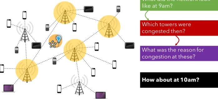
Which towers were congested then?

What was the reason for congestion at these?

How about at 10am?

What did the network look like at 9am?

Figure1.1: Alex, a network administrator, diagnoses issues using data collected in the network.

1

.

1

Motivating Examples

In this section we describe two scenarios, which we will use as running examples throughout this dissertation, to motivate the need for dynamic connected data processing. While the names of the persons used in these examples are fictional, the scenarios depict real world problems faced by enterprise organizations today.

1.1.1

Alex Diagnoses Network Issues

Alex works as a network administrator at a large cellular network operator in the United States. Alex’s job is to manage several thousands of wireless base stations, deployed across a large geographic region, that serves millions of users connect to the Internet every day. Whenever problems occur, and they do occur often in today’s cellular networks, Alex is tasked with finding the reason for the issue and fix them. Monitoring and managing network infrastructure is highly impactful problem for network operators today, with up to USD22billion spent by a single top-tier operator every year in network management

and operation costs. For instance, let’s assume that Alex is trying to find the answer to the question,"What is the reason for poor download throughput for (several) users at9:00am?".

Much like any data driven company today, Alex’s company collects extensive data from their network. The workflow is depicted in fig.1.1. Alex might start with asking

(17)

D D D D D W W D

Were there small deposits & large withdrawals? How many such patterns?

How about in February?

What were the transactions on 01 January?

Figure 1.2: Taylor, a financial analyst, uses transaction data to train a model to detect money laundering.

"How did the network look like at9am?", when the problem actually happened. The query

returns something similar to fig.1.1where there are several base stations serving many

users. Alex doubts congestion as the cuase for low throughput, so the next query is"Which

towers were congested at this point?"that returns a few towers from the original answer.

Then to understand the reason, Alex might run a few machine learning algorithms on the data. Now Alex has to confirm that the findings are indeed correct. To do so, Alex asks

"How about at10am?" meaning to repeat the entire analysis again, but now on a different

subset of the data.

In order to execute these queries and machine learning algorithms on data, Alex uses handwritten scripts to parse and represent the data in a format that is amenable to the analysis, and open source tools such as Scikit Learn [155] or Tensorflow [3] to do the

learning. Unfortunately, Alex faces two issues today. First, the tools available are unable to handle the dynamicityof the data. The network which Alex manages generates several terabytes of data every day, and wading through this massive amount of real-time data is difficult. Second, the tools which Alex uses for analysis do not scale to large datasets, majorly due to the nature of the queries. Thus, Alex spends a significant amount of effort today in doing such analysis.

(18)

1.1.2

Taylor Finds Financial Frauds

Taylor works as a financial analyst at one of the largest banks in the world. A major analysis involved in Taylor’s daily job is in discovering financial frauds. A particular problem of interest for Taylor is money laundering, which accounts for over 200billion

USD every year, and thus an important charter for the bank.

Banks collect extensive information about financial exchanges, and a common ap-proach to finding frauds is to train a machine learning algorithm on these financial transactions to learn a model for detecting fraudulent transaction, and then use this model in real-time transactions to mark suspicious ones. Figure1.2shows how Taylor

does this today, and it starts by retrieving the transactions that took place around the time of known frauds. Once the data is retrieved, Taylor searches for transactions or batches of transactions where small amounts of deposits were made followed by large withdrawals, which is the distinguishing characteristic of classic money laundering. If there are such patterns in the data (there is one such occurrence in fig. 1.2), Taylor gets an

estimate of how many such frauds occurred and retrieves a few of them. These retrieved "laundering patterns" are fed to a learning algorithm which learns a model to detect laundering. Taylor does this process in an ongoing fashion; as new laundering patterns pop-up the model needs to be trained to retain its performance.

Like Alex, Taylor uses a combination of tools to do this analysis; for instance, R [144] for

quickly prototyping and testing some statistical methods, PyTorch [141], TensorFlow [3] or

Python scripts to train the model, and NetworkX [127] or custom programs to discover the

laundering patterns in the data. Similar to Alex’s, Taylor faces the problems ofdynamicity

and scalability, albeit to a much higher extent. Due to the complexity of discovering

patterns in the data, the analysis cannot even handle moderate sized data. Thus, it takes days, or even weeks for Taylor to run the analysis on the data collected by the bank.

1.1.3

Alex & Taylor Aren’t Alone!

Alex and Taylor work with what we refer to in this dissertation asconnected data. In simple terms,connected data is data comprising of entities and their relations. The relations can be explicitly specified (e.g., real-world entities with spatial relations [153] such as base

stations and users in Alex’s case, graphical models [101]) or learned (e.g., raw sensor data

in deep learning tasks [27]). Such data has the power to capture diverse and complex

relations, which could be immensely valuable in many areas including the potential to be the building block of future Artificial Intelligence systems [27].

Indeed, the lives of Alex and Taylor can become much more simpler by the availability of techniques and systems that can operate on large scale dynamic, connected data.

(19)

is limited to Alex and Taylor’s use-cases. The answer is a resounding no. Several emerging applications could benefit from scalable and efficient connected data processing systems. Connected vehicles [35] is an increasingly popular area of interest, both in the industry

and academia. In connected vehicles, connected data processing systems can enable safety systems, such as using the sensor inputs from vehicles and users, combine them with the real-time path taken by vehicles to model impending accidents and provide warnings. Autonomous vehicles are undoubtedly the future of transportation, and we are making huge strides towards achieving this goal. However, managing fleets of autonomous vehicles in the real-world requires extremely robust and scalable traffic flow management systems that can avoid congestion and choke points. Connected data processing systems are likely the foundations in such systems. Finally, with sensors making their ways into our everyday equipment and home automation systems becoming more popular, we are no doubt going to see intelligent smart cities that would enhance our quality of life and the environment. These smart cities would require immense planning, design and ongoing optimizations for efficient operation, and connected data systems would be crucial in understanding how the different entities that constitute the smart city interact with each other and how to optimally actuate the different pieces for achieving the end goal. In short, as the era of Internet-of-Things become reality, the world is moving towards connected data, and systems that can efficient process large scale, dynamic connected data can shape the next generation computation stack.

1

.

2

Problems with Existing Systems

Over the past decade, growing data volumes have pushed the frontiers in large scale data processing and cloud computing. As a result, several cluster processing frameworks exist today that can scale out to a large number of machines and process tremendous amounts of data. The natural question is if these systems can help with dynamic connected data processing. Unfortunately, there are three main challenges that stand in the way of leveraging existing data processing systems for connected data processing.

1.2.1

Programmability

The first challenge is that of programmability. How do we allow end users to query dynamic connected data in a natural and intuitive way? Users like Alex and Taylor are familiar with the simple interface provided by existing Python based tools, and can benefit from similar (simple) interfaces for representing, accessing and manipulating

(20)

Edge Property Vertex Property BS1 UE2 UE1 _BS 2 UE3 UE4 UE5

Figure1.3: Representing connected data as property graphs.

or operating on the data they are interested in. However, no such facilities exist in today’s big data frameworks. While these frameworks provide elegant primitives for unstructured data manipulation, the relation between the entities and the dynamic nature of these relations pose problems. The representation problem is fairly straightforward to address. At a given point in time, connected data depicts the state of entities and their relations. Such relations are naturally represented asgraphs. For instance, Alex’s network can be represented by a property graph (§2.2.1) where the entities in the network, such

as users and base stations, are graphnodesas shown in fig. 1.3. We follow this natural

representation format in this dissertation and thusdynamicconnected data is represented

asdynamic property graphs (§3.3.1). Unfortunately, efficient storage and operations on

dynamic graphs are still open questions.

1.2.2

Storage

Connected data analysis isdata intensive, as we saw with the examples of Alex and Taylor. In both these scenarios, data is generated in the order of several terabytes every day. The volume of data is only poised to increase with emerging Internet-of-Things applications, for instance, autonomous/connected vehicles are expected to generate over4terabytes

of data per day by2020[83]. Thus, efficiently storing and retrieving large quantities of

dynamic connected data is a huge challenge. This is because commonly used techniques in databases such as building indices for improving the access efficiency is not possible in connected data processing.

1.2.3

Performance

Extracting performance in the face of dynamicity forms the biggest challenge in connected data analysis. Most of connected data queries are both interactiveandexploratory. They

(21)

waitingfor the results. Theexploratorynature is because the queries are executed based on what the user sees; the answer to a query determines the next query. Thus, queries are executed in anad-hocfashion, and are not predetermined. In such scenarios, performance optimization techniques such as pre-processing and query specific caching do not help.

1

.

3

Solution Overview

This dissertation focuses on the core problems in realizing efficient dynamic connected data processing systems. Towards this goal, we design and implement the following systems:

Tegra focuses on the problem ofad-hoc analyticson dynamic connected data. It aims to solve the problems faced by Alex and Taylor and forms the foundation for the other systems. To do so, it represents dynamic connected data as dynamic/evolving property graphs, and proposes techniques for efficient storage and ad-hoc window operations on evolving graphs. It enables efficient access to the state of the graph at arbitrary windows, and significantly accelerates ad-hoc window queries by using a compact in-memory representation for both graph and intermediate computation state. For this, it leverages persistent datastructures to build a versioned, distributed graph state store, and couples it with an incremental computation model which can leverage these compact states. For users, it exposes these compact states using Timelapse, a natural abstraction. Te g r a

significantly outperforms other systems (by up to30×) for ad-hoc window operations.

ASAPspecifically focuses on usecases similar to Taylor’s roadblock, the intractability of scaling pattern discovery queries to larger datasets, and proposes a fast, approximate computation engine for graph pattern mining. It leverages state-of-the-art results in graph approximation theory, and extends it to general graph patterns in distributed settings. To enable the users to navigate the tradeoff between the result accuracy and latency, we propose a novel approach to build the Error-Latency Profile (ELP) for a given computation. A S A P outperforms existing exact pattern mining solutions by orders of magnitude. Further, it can scale to graphs with billions of edges without the need for large clusters.

GAP explores the question of applying approximation to the problem of iterative analytics on connected data and takes a first attempt at realizing approximate graph analytics engine. Here, we discuss how traditional approximate analytics techniques do not carry over to the graph usecase. Leveraging the characteristics of graph properties and algorithms, GAP proposes a graph sparsification technique, and a machine learning

(22)

based approach to choose the apt amount of sparsification required to meet a given budget.

Monarchattempts to enhance the connected data processing systems by looking at making them function when deployed in a geo-distributed fashion and thus focuses on the problem of efficient geo-distributed graph analytics. We find that optimizing the iterative processing style of graph-parallel systems is the key to achieving this goal rather than extending existing geo-distributed techniques to graph processing.

CellScope looks at the fundamental difficulties in making real-time decisions on real-time connected data. Such real-time decision tasks include simple reporting on data streams to sophisticated model building. We observe that the practicality of these analyses are impeded in several domains because they are faced with a fundamental trade-off between data collection latency and analysis accuracy. To solve this issue, we look at one particular domain, Alex’s network performance diagnosis, to study the trade-off in detail and find that the trade-off can be resolved using two broad, general techniques: intelligent data grouping and task formulations that leverage domain characteristics. Based on this, Ce l lSc o p e applies a domain specific formulation and application of

Multi-task Learning(MTL) to network performance analysis. It uses three techniques: feature engineering to transform raw data into effective features, a PCA inspired similarity metric to group data from geographically nearby base stations sharing performance commonalities, and a hybrid online-offline model for efficient model updates. We then generalize the techniques and show their efficacy in other domains.

1

.

4

Dissertation Plan

This dissertation is organized as follows. Chapter2 provides background on large scale

data processing. Chapter3describes the work on supporting ad-hoc analytics on dynamic

connected data. We discuss Te g r a here, which proposes efficient ways to store and

per-form ad-hoc window operations. In chapter 4, we focus on pattern mining on connected

data, looking at problems such as Taylor’s. We describe A S A P in this chapter, which is a fast, approximate pattern mining system that achieves several orders of magnitude improvement over the state of the art techniques. Chapter 5 attempts to extend the

learning from ASAP to iterative analytics, and describes GAP, an approximate analytics engine. We discuss how connected data is naturally generated in a geo-distributed fashion and attempt to extend connected data processing systems to geo-distributed settings by describing Mo n a r c h in chapter6. Chapter 7 looks at the fundamental trade-offs in

making real-time decisions on dynamic connected data and describes Ce l lSc o p e, our

(23)

Chapter

2

Background

In this dissertation, we follow the natural representation format of viewing (dynamic) connected data as (dynamic) property graphs (§1.2.1). Thus, the systems we discuss in

the following chapters build on the rich distributed graph processing literature. To aid the reader in following the rest of the dissertation, we begin with a brief background on large scale data processing systems, focusing on data-parallel and graph parallel systems.

2

.

1

Data Parallel Processing

Over the last decade, data parallel systems have gained popularity for processing large amounts of data. These systems were aimed at simplifying parallel computation over large amounts of distributed data. Typically, these systems expose simple abstractions and operators that developers use to achieve the desired processing goals, and internally manage the intricacies of efficiently running these operations on the data in parallel.

The most popular early proposal in this space is Google’s MapReduce [52], which

exposed just two operators—map and reduce—that could capture many embarrassingly

paralleluse-cases such as rebuilding Google’s search indexes, the use-case it was originally

intended for, and provided efficient execution in a fault-tolerant fashion. The tremendous popularity of MapReduce resulted in the emergence of a large number of systems [84, 190, 125, 193, 192, 21] and sparked research in many core areas such as scheduling,

query optimization and programming models. The new generation engines, such as Naiad [125], Spark [192] and Flink [21], improved upon the original MapReduce proposal

by incorporating new operators, declarative interfaces, better task execution plans and in-memory caching to reduce inefficiencies with intermediate data management.

Traditionally, most of the dataflow engines were targeted at processing batches of unstructured data. However, as new application scenarios emerged, they have increasingly

(24)

incorporated new functionalities such as the ability to do graph processing [115, 22, 71],

stream processing [21, 13,194] and machine learning [102, 162].

2

.

2

Graph Parallel Processing

We discuss graph parallel processing in this section, touching upon representation, abstractions and optimizations.

2.2.1

Property Graph Model

Graph processing systems typically represent graph structured data as a property graph [148], which associates user-defined properties with each vertex and edge. The

properties can include meta-data (e.g., user profiles and time stamps) and program state (e.g., the number of neighbors, or rank of vertices). For example, fig. 1.3 shows Alex’s

network at a particular instance in time (say 9:00am) as a property graph. Here, the

vertices (users and base stations) can hold properties such as the total data transferred and number of users active while the edges can be made to store properties specific to the node pairs such as signal quality, geographical distance and so on. This enables Alex to query and filter the network based on properties and thus create analysis specific instances of graphs as input to the next stage of processing.

Property graphs are logically represented in a distributed dataflow framework such as MapReduce [52] as a pair of vertex and edge property collections, where the collections

contain the mapping between the vertex or edge and their properties. This enables the composition of graphs with other collections in the dataflow frameworks [71]. An

alternative to property graphs for associating data with graph entities is the Resource Description Framework (RDF) format [148] which stores triplets of

subject-predicate-object. However, compared to RDF, property graphs are considered to be a better format for storage and querying, especially for graph analytics.

2.2.2

Graph Parallel Abstractions

Most existing general purpose graph processing systems allow end-users to perform graph computations by exposing agraph-parallelabstraction. A graph-parallel abstraction consists of a graph and a vertex-program, provided by the user, which is executed in parallel on each vertex. The program running on individual vertex can interact with the vertex’sneighborhood. This interaction between vertices is implemented using either shared state (e.g., GraphLab [111]) or message passing (e.g., Pregel [115]). Each vertex

(25)

halt the program terminates.

Pregel

Pregel [115] proposes aBulk Synchronous Parallel (BSP)message passing abstraction where

all the vertex programs run simultaneously in a series of super-steps. In every super-step, each vertex program receives all messages from the previous super-step and sends messages to its neighbors in the next super-step. At the end of each super-step, a barrier is imposed in order to ensure that all the vertex programs finish processing messages before proceeding to the next. This ensures program correctness (at the cost of efficiency). A Pregel program terminates when there are no messages remaining to be sent and every vertex program has voted to halt. Pregel exposes several optimizations to improve the efficiency of the message passing, for instance, messages destined to the same vertex are combined using a commutative associative user-defined function.

GraphLab

GraphLab [111] proposes anasynchronous distributed shared-memoryabstraction where the

vertex programs have shared access to the distributed graph. Each vertex program access information about the current and adjacent vertices and edges directly and no message passing is involved. In this model, correctness of the program is ensured by the GraphLab system by serializing the program execution at neighbors. GraphLab eliminates messages and also synchronization and can thus achieve higher efficiency by isolating and handling data movements at the system level. However, this comes at the cost of an increased complexity, and the gains due to an asynchronous programming model are often offset by this additional complexity. Thus, a majority of distributed graph processing systems today adopt the bulk synchronous model.

GAS Decomposition

PowerGraph [70] observes that while Pregel and GraphLab differ in how they collect

and distribute information, they share a common structure. Thus, it proposes the Gather-Apply-Scatter (GAS) decomposition to characterize this common structure and differentiate between vertex and edge specific computations. The GAS model captures the conceptual phases of the vertex program as shown in listing 2.1. In the GAS

de-composition, a vertex program consists of three data parallel phases: a gather phase that collects information about adjacent vertices and edges and applies a function on them, the apply phase that uses the function’s output to update the vertex, and the

(26)

def Gather(u, v) = Accum

def Apply(v, Accum) = vnew

def Scatter(v, j) = jnew, Accum

Listing 2.1: The Gather-Apply-Scatter (GAS) decomposition introduced in PowerGraph [70].

scatter phase that uses the new vertex value to update adjacent edges. The system executes these phases sequentially. Since the GAS decomposition leads to a pull based model of message computation, it enables vertex-cut partitioning, and improved work balance which are essential in achieving performance in real-world graphs which follow power-law distribution [70]. As a result, many popular open-source graph-processing

(27)

Chapter

3

Ad-Hoc Analytics on Dynamic

Connected Data

3

.

1

Introduction

In this chapter, we focus on the problem ofefficient ad-hoc window operations on dynamic connected data represented as evolving graphs—the ability to perform ad-hoc queries on arbitrary time windows (i.e., segments in time) either in the past or in real-time. The motivating examples described in the previous chapter (§1.1) are indeed instances of such

exploratoryanalysis.

Alex’s transient failure diagnosis started by retrieving a series of snapshots1 of the

network represented as an evolving graph before and after the failure. The process then

involved running a handful of queries on the retrieved window, and then iteratively refining the queries until a hypothesis could be formed. The process culminating with the repetition of thesamequeries on a different window. Similarly, Taylor’s quest towards discovering money laundering involved improving the fraud detection algorithm by retrieving thecomplete states of the transaction graph at different segments in timeto train and test variants of the algorithm. In such scenarios, neither the queries nor the windows on which the queries would be run are predetermined.

To efficiently perform ad-hoc window operations, a graph processing system should provide two key capabilities. First, it must be able to quickly retrieve arbitrary size windows starting at arbitrary points in time. There are two approaches to provide this functionality. The first is to store asnapshotevery time the graph is updated, i.e., a vertex or edge is added or deleted. While this allows one to efficiently retrieve the state of

1

A snapshot is a full copy of the graph, and can be viewed as a window of size zero. Non-zero windows have several snapshots.

(28)

the graph atanypoint in the past, it can result in prohibitive overhead. An alternative is to store only the changes to the graph and reconstruct a snapshot on demand. This approach is space efficient, but can incur high latency, as it needs to re-apply all updates to reconstruct the requested snapshot(s). Thus, there is a fundamental trade-off between in-memory storage and retrieval time.

Second, we must be able to efficiently execute queries (e.g., connected components) not only on a single window, but also across multiple related windows of the graph. Existing systems, such as Chronos [76] allows executing queries on a single window,

while Differential Dataflow [125] supports continuously updating queries over sliding

windows. However, none of the systems support efficient execution of queries across multiple windows, as they do not have the ability to share the computation state across windows and computations. This fundamental limitation of existing systems arises from their inability to efficiently store intermediate state from within a query for later reuse.

We present Te g r a2, a system that enables efficient ad-hoc window operations on

time-evolving graphs. Te g r a is based on two key insights about such real-world evolving

graph workloads: (1) during ad-hoc analysis graphs change slowly over time relative to their

size , and (2) queries are frequently applied to multiple windows relatively close by in time.

Leveraging these insights Te g r a is able to significantly accelerate window queries by

reusing both storage and computation across queries on related windows. Te g r a solves

the storage problem through a highly efficient, distributed, versioned graph state store

which compactly represents graph snapshots in-memory as logically separate versions that are efficient for arbitrary retrieval. We design this store using persistent data-structures that lets us heavily share common parts of the graph thereby reducing the storage requirements by several orders of magnitude (§3.5). Second, to improve the

performance of ad-hoc queries, we introduce an efficient in-memory representation of intermediate state that can be stored in our graph state store and enables non-monotonic3

incremental computations. This technique leverages the computation pattern of the familiar graph-parallel models to create compact intermediate state that can be used to eliminate redundant computations across queries. (§3.4).

Te g r a exposes these compact persistent snapshots of the graph and computation

state using a logical abstraction named Timelapse, which hides the intricacies of state management and sharing from the developer. At a high level, a timelapse is formed by a sequence of graph snapshots, starting from the original graph. Viewing the time-evolving graph as consisting of a sequence of independent static snapshots of the entire graph makes it easy for the developer to express a variety of computation patterns naturally,

2

forTimeEvolvingGRaphAnalytics. 3

Allows vertex/edge deletions, additions and modifications on any graph algorithm implemented in a graph-parallel fashion.

(29)

efficient incremental computations (§3.3.1). Finally, since Timelapse is backed by our

persistent graph store, users and computations always work on independent versions

of the graph, without having to worry about consistency issues. Te g r a outperforms

existing systems by up to30×on ad-hoc window operation workloads (§3.7).

In summary, we make the following contributions:

• We present Te g r a, a time-evolving graph processing system that enables efficient

ad-hoc window operations on both historic and live data. To achieve this, Te g r a shares

storage, computation and communication across queries by compactly representing the evolving graph and intermediate computation state in-memory.

• We proposeTimelapse, a new abstraction for time-evolving graph processing. Te g r a

exposes timelapse to the developer using a simple API that can encompass many time-evolving graph operations. (§3.3.1)

• We design(DGSI), an efficient distributed, versioned property graph store that enables timelapse APIs to perform efficient operations. (§3.5)

• Leveraging timelapse and DGSI, we present an iterative, incremental graph computa-tion model which supports non-monotonic computacomputa-tions. (§3.4)

3

.

2

Background & Challenges

3.2.1

Time-evolving Graph Workloads

Time-evolving graph workloads, an important graph workload [153], can be of three

categories:

Temporal Queries: Here, an analyst is querying the graph at different points in the past and evaluates how the result changes over time. Examples are “How many friends did

Alice have in 2017?” or “How did Alice’s friend circle change in the last three years?”. Such

queries may have time windows of the form [T−δ, T] and are performed on offline data, and are executed in batch.

Streaming/Online Queries: These workloads are aimed at keeping the result of a graph computation up-to-date as new data arrives (i.e., [Now−δ,Now]). For example, the analyst may ask“What are the trending topics now?”, or use a moving window (e.g.,“What

are the trending topics in the last10minutes?”). These queries focus on the most recent data,

(30)

Ad-hoc Queries: In these workloads, an analyst is likely to explore the graph by performing ad-hoc queries on arbitrary windows. For example, consider the exact queries used by Alex (§1.1), a network administrator troubleshooting a transient failure that

occurred at09:00AM. To do so, Alex may ask“What were the hotspots at08:00AM?”which

runs a connected component algorithm on the snapshot. Based on what is seen, the next query may ask “What were the hotspots at10:00AM?”followed by“At10:00AM, what is the

shortest path of hotspot X to the controller?”. Alex iteratively refines this query by taking

many snapshots and running the query. In another example, Taylor, a financial expert is interested in improving the fraud-detection algorithm4

. Taylor queries“Who were the

top influencers1month around April1?” which retrieves the window of1month around a

known fraud and runs an algorithm (e.g., personalized page rank) on the window, and then launches follow-up queries based on what the output is. Taylor repeats this on different windows to learn new rules that would detect the fraud. Taylor then tests her changes on a different set of windows, possibly also with injecting artificial data.

In ad-hoc workloads, not only does the analyst need to access arbitrary windows, but also the queries and the windows on which they are executed are determined just-in-time (i.e., not predetermined). Further, the analyst applies the same query to multiple (close-by, discontinuous) windows.

3.2.2

Limitations of Existing Solutions

Recent work in graph systems has made considerable progress in the area of evolving graph processing. (§3.8)

Temporal analysis engines (e.g., Chronos [76], ImmortalGraph [120]) operate onoffline data and focus on executing queries on one or a sequence of snapshots in the graph’s history. Upon execution of a query, these systems load the relevant history of the graph and utilize a pre-processing step to create an in-memory layout that is efficient for analysis. Such preprocessing can often dominate the algorithm execution time [116].

As a result, these systems are tuned for operating on a large number of snapshots in each query (e.g., temporal changes over months or year), and are efficient in such cases. Fundamentally, the in-memory representation in these systems cannot support updates. Additionally, these systems do not allow updating the results of a query.

Streaming systems (e.g., Kineograph [45], DifferentialDataflow [119], Kickstarter [175],

GraphBolt [117]) operate onlive dataand allow query results to be updatedincrementally

(rather than doing a full computation) when new data arrives. These systems only allow queries on the live graph, and do not support ad-hoc retrieval of previous state.

4

(31)

cannot be utilized over multiple windows. Further, most systems (with the exception of Differential Dataflow, to the best of our knowledge) do not support non-monotonic

computations in their incremental model, and either assume some properties of the algorithm, or leave it up to the developer to ensure correctness.

Differential Dataflow (DD) allows general, non-monotonic incremental computations using special versions of operators. Each operator stores “differences” to its input and produces the corresponding differences in output (hence full output is not materialized), automatically incrementalizing algorithms written using them. While this technique is very efficient for real-time streaming queries, incorporating ad-hoc window operations in it is fundamentally hard. Since the computation model is based on the operators maintaining state (differencesto their input and output) indexed by data (rather than time), accessing a particular snapshot can require a full scan of the maintained state. Further, since every operator needs to maintain state, the system accumulates large state over time which must be compacted (at the expense of forgoing the ability to retrieve the past). Finally, intermediate state of a query is cleared once it completes and storing these efficiently for reuse is an open question5

.

3.2.3

Challenges

Meeting the requirements necessary to support efficient ad-hoc window operations in practice is hard. There are three main challenges that stand in the way of building such a system. First is that ofprogrammability. The system must be able to provide the end user a natural and intuitive way to operate on time-evolving graphs. Second, the system must support efficientstorageof evolving graphs. While it is ideal to store the history of the graph as individual snapshots for zero overhead ad-hoc retrieval, but the system needs to consider the storage overhead due to duplication with every snapshot stored. Finally, ad-hoc analytics is both interactive (the user is waiting for answers) and exploratory (new queries are based on the answers to previous ones) and thus, extracting performanceunder these constraints is difficult. To accelerate queries across windows, the system must not only be able to store intermediate states efficiently, but also be able to leverage them in its computation model. In essence, it must be able to compactly represent and share data and state between queries across multiple windows and users.

5

Our conversations with the author of DD revealed that incorporating the state management techniques we propose in this work in DD is fundamentally hard and requires modification of its execution engine.

(32)

3

.

3

Tegra Design

Our solution, Te g r a, consists of three components:

Timelapse Abstraction (§3.3.1): In Te g r a, users interact with time-evolving graphs

us-ing thetimelapseabstraction, which logically represents the evolving graph as a sequence

of static,immutable graph snapshots. Te g r a exposes this abstraction via a simple API

that allows users to save/retrieve/query the materializedstateof the graph at any point.

Computational Model (§3.4): Te g r a proposes a computation model that allowsad-hoc

queries across windows to share computation and communication. The model stores

com-pact intermediate state as a timelapse, and uses it to perform general, non-monotonic

incremental computations.

Distributed Graph Snapshot Index (§3.5): Te g r a stores evolving graphs, intermediate

computation state and results in DGSI, an efficient indexed, distributed, versioned property graph store whichshares storagebetween versions of the graph. In fact, Timelapse can be seen as “views” on the data stored in DGSI. Such decoupling of state from queries and operators allow Te g r a to share it across queries and users.

3.3.1

Timelapse Abstraction & API

Te g r a introduces Timelapse as a new abstraction for time-evolving graph processing

that enables efficient ad-hoc analytics. The goal of timelapse is to provide the end-user with a simple, natural interface to run queries on time-evolving graphs, while giving the system opportunities for efficiently executing those queries. In timelapse, Te g r a logically

represents a time-evolving graph as a sequence of immutable, static graphs, each of which we refer to as snapshotin the rest of this chapter. A snapshot depicts a consistent state of the graph at a particular instance in time. Te g r a uses the popular property graph

model [71], where vertices and edges in the graph are associated with arbitrary properties,

to represent each snapshot in the timelapse. For the end-user, timelapse provides the abstraction of having access to amaterializedsnapshot at any point in the history of the graph. This enables the usage of the familiar static graph processing model in evolving graphs (e.g., queries on arbitrary snapshot).

Timelapses are created in Te g r a in two ways—by the system and by the users. When

a new graph is introduced to the system, a timelapse is created for it that contains a single snapshot of the graph. Then, as the graph evolves, more snapshots are added to the timelapse. Similarly, users may create timelapses while performing analytics. Because

(33)

ID can be autogenerated. Returns the id of the saved snapshot.

retrieve(id): snapshot Return one or more snapshots from the timelapse. Allows simple matching on the id.

diff(snapshot, snapshot): delta Difference between two snapshots in the timelapse. (§3.4) expand(candidates): subgraph Given a list of candidate vertices, expand the computa-tion scope by marking their1-hop neighbors. Used for implementing incremental computations ( §3.4)

merge(snapshot,snapshot,func): snapshot

Create a new snapshot using the union of vertices and edges of two snapshots. For common vertices, run func to compute their value. Used for implementing incremental computations ( §3.4)

Table3.1: Te g r a exposes Timelapse via simple APIs.

snapshots in a timelapse are immutable, any operation on them creates new snapshots as a result (e.g., a query on a snapshot results in another snapshot as a result). Such newly created snapshots during an analytics session may be added to an existing timelapse, or create a new one depending on the kind of operations performed. For instance, for an analyst performing what-if analysis by introducing artificial changes to the graph, it is logical to create a new timelapse. Meanwhile, snapshots created as a result of updating a query result should ideally be added to the same timelapse. The system does not impose restrictions on how users want to book-keep timelapses. Instead, it simply tracks their lineage and allows users to efficiently operate on the timelapses. (§3.5)

Since timelapse logically represents a sequence of related graph snapshots, it is intuitive to expose the abstraction using the same semantics as that of static graph. In Te g r a, users interact with timelapses using a language integrated API. The API extends

the familiarGraphinterface, common in static graph processing systems, with a simple set of additional operations, listed in table3.1. This enables users to continue using existing

static graph operations on any snapshot in the timelapse obtained using theretrieve()

API.

3.3.2

Evolving Graph Analytics Using Timelapse

The natural way to do graph computations over the time dimension is to iterate over a sequence of snapshots. For instance, an analyst interested in executing thedegreesquery on three snapshots,G1, G2 and G3 depicted in fig. 3.1can do:

for(id <- Array(G1,G2,G3))

(34)

D

BC

BA

AA

A

B

C

A

B

C

D

A

B

C

D

E

Time

G

1

G

2

G

3

A

B

C

D

E

Figure3.1: A timelapse of graph Gconsisting of three snapshots. For temporal analytics, instead of applying graph-parallel operations independently on each snapshot (left), timelapse enables them to be applied to all snapshots in parallel (right).

However, applying the same operation on multiple snapshots of a time-evolving graph independently is inefficient. In graph-parallel systems (§3.2),_degrees₍₎ computation is

typically implemented using a user-defined program where every vertex sends a message with value1to their neighbors, and all vertices adding up their incoming message values. Such message exchange accounts for a non-trivial portion of the analysis time [154]. In the

earlier example, sequentially applying the query to each snapshot results in11messages

of which5are duplicates (fig. 3.1).

To avoid such inefficiencies, timelapse allows access to the lineageof graph entities. That is, it provides efficient retrieval of the state of graph entities in any snapshot. Using this, graph-parallel phases can operate on the evolution of an entity (vertex or edge) as opposed to a single (at a given snapshot) value. In simple terms, each processing phase is able to see the history of the node’s property changes. This allows temporal queries (§3.2.1) involving multiple snapshots, such as the degree computation, to be efficiently

expressed as:

results = G.degrees(Array(G1,G2,G3))

wheredegrees implementation takes advantage of timelapse by combining the phases in graph-parallel computation for these snapshots. That is, the user-defined vertex program is provided with state in all the snapshots. Thus, we are able to eliminate redundant messages and computation.

(35)

1 A B A 1 B A B 2 B A A

A

B

C

B

C

A

B

A

G

₁

G

2

R

2

A

B

C

G

2

A

B

R

3

A

R

₁ A B B C A A B A A A B B

1

2

3

Figure 3.2: 1 Connected components by label propagation on snapshot G₁ produces

R1. 2 Vertex A and edge A−B is deleted in G₂. Using the last result to bootstrap

computation results in incorrect answer R2. 3 A strawman approach of storing all

messages during the initial execution and replaying it produces correct results, but needs to store large amounts of state.

3

.

4

Computation Model

To improve interactivity, Te g r a must be able to efficiently execute queries by effectively

reusing previous query results to reduce or eliminate redundant computations, commonly referred to as performingincremental computation. Here, we describe Te g r a’s incremental

computation model.

3.4.1

Incremental Graph Computations

Supporting incremental computation requires the system to managestate. The simplest form of state is the previous computation result. However, many graph algorithms are iterative in nature, where the graph-parallel stages are repeatedly applied in sequence until a fixed point. Here, simply restarting the computations from previous results do not lead to correct answers. To illustrate this, consider a connected components algorithm using label propagation on a graph snapshot, G₁ as shown in 1 in fig.3.2which entails

result R1 after three iterations. When the query is to be repeated onG2, restarting the

computation fromR1 as shown in 2 computes incorrect result. In general, correctness in

such techniques depend on the properties of the algorithm (e.g., abelian group) and the monotonicity of updates (e.g., the graph only grows).

(36)

Supporting general non-monotonic iterative computations require maintaining

inter-mediatestate. In the previous example, one solution is to store every message exchanged

between graph entities during the initial execution of the algorithm. When the query is executed on the updated graph, the system can selectively replay these stored messages to ensure correctness of the results as depicted in 3 . However, this approach requires

stor-ing and effectively usstor-ing large amounts of state (proportional to the number of edges for every iteration), which may pose prohibitive overheads when applied to real-world graphs where the number of edges are significantly more compared to vertices [70]. Further, the

state is tied to the computation performed and thus doesn’t provide opportunities to share it across queries.

Te g r a proposes a general, incremental iterative graph-parallel computation model

that significantly reduces the state requirements. It leverages the fact that graph-parallel computations proceed by making iterative changes to the original graph. Thus,iterations of

a graph-parallel computation can be seen as a time-evolving graph, where the snapshots are the

materialized state of the graph at the end of each iteration. Since timelapse can efficiently store and retrieve these snapshots, we can perform incremental computations without the need to store the message exchanges. We call this modelIncremental Computation by

entity Expansion(ICE).

3.4.2

ICE Computation Model

ICE executes computations only on the subgraph that would be affected by the updates

at each iteration. To do so, it needs to find the relevant entities that should participate in

computation at any given iteration. For this, it uses the state stored as timelapse, and the computation proceeds in four phases:

Initial execution: When an algorithm is executed for the first time, ICE stores the state of the vertices (and edges if the algorithm demands it) as properties in the graph. At the end of every iteration, a snapshot of the graph is added to the timelapse. The ID is generated using a combination of the graph’s unique ID, an algorithm identifier and the iteration number. As depicted in 1 in the examples in fig. 3.3, the timelapse contains

three and four snapshots, respectively.

Bootstrap: When the computation is to be executed on a new snapshot, ICE needs to bootstrap the incremental computation. Intuitively, the subgraph that must participate in the computation at bootstrap consists of the updates to the graph, and theentities affected

by the updates. For instance, any newly added or changed vertices should be included.

Similarly, edge modifications would result in the source and/or destination vertices to be included in the computation. However, the changes alone are not sufficient to ensure correctness of the results. This is because in graph-parallel execution, the state of a

(37)

A B C A A B A A A A B C A A B A 1 G1 0 G1 1 G1 2 A B C D G2 0 A A B A G2 1 A A A A G2 2 D A A A 2 3 4 B D E 1 A C B B D A A B A B A A A A A A A B D E A C B B D C B B B B B B B B G1 0 G1 1 G1 2 G1 3 G2 0 G2 1 G2 2 2 3 3 4 G2 3 Figure 3 . 3 : T w o examples that depict ho w ICE w orks. Dotted cir cles indicate v ertices that recompute, and double cir cles indicate v ertices that need to be pr esent in the subgraph to compute the corr ect answ er , but do not recompute state themselv es. 1 Iterations of initial execution is stor ed in the timelapse. 2 ICE bootstraps computation on a ne w snapshot, b y finding the subgraph consisting of af fected v ertices and their dependencies (neighbors). In the second example, C is af fected b y the deletion of A − C . T o recompute state it nee ds D (yields subgraph C − D ). 3 At ev er y iteration, after execution of the computation on the subgraph, ICE copies state for entities that did not recompute. Then finds the ne w subgraph to compute b y comparing the pr evious subgraph the timelapse snapshot. In the second example, though C recomputes the same v alue as in pr evious iteration, its state is dif fer ent fr om the snapshot in timelapse and hence needs to be pr opagated. 4 ICE ter minates when the subgraph conv er ges and no entity in the graph needs the state copied fr om stor ed snapshots in the timelapse.

(38)

graph entity is dependent on the collective input from its neighbors. Thus, ICE must also include the one-hop neighbors ofaffected entities, and so the bootstrapped subgraph consists of the affected entities and their one-hop neighbors. ICE uses theexpand() API for this purpose. The graph computation is run on this subgraph. The first example’s 2

in fig.3.3shows how ICE bootstraps when a new vertexDand a new edge between A

andDis added. DandAshould recompute state, but for Ato compute the correct state, it must involve its one-hop neighborB, yielding subgraphD−A−B.

Iterations: At each iteration, ICE needs to find the right subgraph to perform computa-tions. ICE exploits the fact that the nature of the graph-parallel abstraction restricts the propagation distance of updates in an iteration. Intuitively, the graph entities that might possibly have a different state at any iteration will be contained in the subgraph that ICE has already executed computation on from the last iteration. Thus, after the initial bootstrap, ICE can find the new subgraph at a given iteration by examining the changes to the subgraph from the previous iteration and expanding to the one-hop neighborhood of affected entities. For the vertices/edges that did not recompute the state, ICE simply copies the state from the timelapse. In 3 in fig. 3.3 (first example), though A and D

recomputed, onlyDchanged state and needs to be propagated to its neighbor Awhich needsB.

Termination: It is possible that modifications to the graph may result in more (or less) number of iterations compared to the initial execution. Unlike normal graph-parallel computations, ICE does not necessarily stop when the subgraph converges. If there are more iterations stored in the timelapse for the initial execution, ICE needs to check if the unchanged parts of the graph must be copied over. Conversely, if the subgraph has not converged and there are no more corresponding iterations, ICE needs to continue. To do so, it simply switches to normal (non-incremental) computation from that point. Thus, ICE converges only when the subgraph converges and no entity needs their state to be copied from the stored snapshot in the timelapse. (4 in fig.3.3)

3.4.3

ICE vs Streaming Systems

ICE provides several desirable properties for ad-hoc exploratory analysis on evolving graphs, and differs from the computation models in existing streaming graph processing systems (e.g., Differential Dataflow, Kickstarter, GraphBolt) in two major ways. First, the state in ICE model is decoupled from computation, and ICE generates the exact same intermediate states as a system that executes the algorithm from scratch (i.e., non-incremental computation) at every iteration. In addition to guaranteeing the correctness even for non-monotonic computations, this allows ICE to leverage any user specified previous state for incremental computations compared to streaming systems which can