The Collateral Channel:
How Real Estate Shocks affect Corporate Investment
∗
Thomas Chaney
†David Sraer
‡David Thesmar
§August 15, 2011
Abstract
What is the impact of real estate prices on corporate investment? In the presence of financing frictions, firms use pledgeable assets as collateral to finance new projects. Through this collateral channel, shocks to the value of real estate can have a large impact on aggregate investment. Over the 1993-2007 period, the representative U.S. corporation invests $.06 out of each $1 of collateral. To compute this sensitivity, we use local variations in real estate prices as shocks to the collateral value of firms that own real estate. We address the endogeneity of local real estate prices using the interaction of interest rates and local constraints on land supply as an instrument. We address the endogeneity of the decision to own land (1) by controlling for observable determinants of ownership and (2) by looking at the investment behavior of firms before and after they acquire land. The sensitivity of investment to collateral value is stronger the more likely a firm is to be credit constrained.
∗We are grateful to Institut Europlace de Finance for financial support. For their helpful comments, we
would like to thank Nicolas Coeurdacier, Stefano DellaVigna, Denis Gromb, Luigi Guiso, Thierry Magnac, Ulrike Malmendier, Atif Mian, Adam Szeidl and Jean Tirole, as well as two anonymous referees and the Editor. We are especially indebted to Chris Mayer, for providing us with the Global Real Analytics data. We are also grateful to seminar participants at INSEE in Paris, USC, UC San Diego Rady School of Management, NYU Stern, MIT Sloan, the University of Amsterdam, London Business School, Oxford’s Saïd School of Business, the University of Chicago, the European University Institute in Florence, Bocconi University, Toulouse School of Economics, the Kellogg School of Management, Princeton University, the Haas School of Business at Berkeley, and the University of Naples. We are solely responsible for all remaining errors.
†University of Chicago, NBER and CEPR,[email protected]
‡Princeton University, [email protected]. Corresponding Author: 26 Prospect Avenue, Princeton, NJ
08540.
1
Introduction
In the presence of contract incompleteness, Barro (1976), Stiglitz and Weiss (1981) and Hart and Moore (1994) point out that collateral pledging enhances a firm’s debt capacity. Providing
outside investors with the option to liquidate pledged assetsex post acts as a strong disciplining
device on borrowers. This, in turn, eases financing ex ante. Asset liquidation values thus
play a key role in the determination of a firm’s financing capacity. This simple observation has important macroeconomic consequences: as noted by Bernanke and Gertler (1989) and Kiyotaki and Moore (1997), business downturns will deteriorate assets values, thus reducing debt capacity and depressing investment, which will amplify the downturn. This “collateral channel” is often the main suspect for the severity of the Great Depression (Bernanke (1983)) or for the extraordinary expansion of the Japanese economy at the end of the 80’s (Cutts (1990)). In the current context of abruptly declining real estate prices in the U.S., an assessment of the relevance of this “collateral channel” is called for. This paper attempts to empirically uncover
the microeconomic foundation for this mechanism.
We show that over the 1993-2007 period, a $1 increase in collateral value leads the rep-resentative U.S. public corporation to raise its investment by $.06. This sensitivity can be quantitatively important in the aggregate. This is because real estate represents a sizable frac-tion of the tangible assets that firms hold on their balance sheet. As we show in this paper, in 1993, among public firms in the US, 58% reported at least some real estate ownership. Among these land-owning firms, our estimation of the value of real estate holdings represented some 20% of shareholder value.
To get at this $.06 sensitivity, we use variations in local real estate prices, either at the state or the city level, as shocks to the collateral value of land holding firms. We measure how a firm’s
investment responds to each additional dollar of real estate that the firmactually owns, and not
how investment responds to real estate shocks overall. This empirical strategy uses two sources of identification. The first comes from the comparison, within a local area, of the sensitivity of investment to real estate prices across firms with and without real estate. The second comes from the comparison of investment by land holding firms across areas with different variations in real estate prices. The methodology is similar to Case et al. (2001) in their study of home wealth effects on household consumption.
Two sources of endogeneity might affect our estimation. First, real estate prices may be correlated with the investment opportunities of land holding firms. We instrument local real estate prices using the interaction of long-term interest rates (to capture time variations in housing demand) with local housing supply elasticity (see Himmelberg et al., 2005, and Mian and Sufi, 2009, for a use of these elasticities). The second endogeneity issue is that the decision to own or lease real estate may be correlated with the firm’s investment opportunities or the extent of its credit constraints (Eisfeldt and Rampini, 2009, and Rampini and Vishwanathan, 2010). We do not have a proper set of instruments to deal with this problem, but we make two attempts at gauging the severity of the bias it may cause. We first control for the observable determinants in the ownership decision, which leaves the estimation unchanged. Second, we estimate the sensitivity of investment to real estate prices for firms that acquire real estate
before and after they do so. Before acquiring real estate, future purchasers are statistically
real estate prices becomes large, positive and significant only after they acquire real estate. This paper is a contribution to the emerging empirical literature on collateral and investment. The seminal paper in this literature is Peek and Rosengreen (1997), who look at the supply side of credit. During the collapse of the Japanese real estate bubble in the early 1990s, they show that banks owning depreciated real estate assets cut their credit supply in the US, leading to
a decrease in their clients’ investment.1 Closest to our paper is Jie Gan (2007a) who shows
that land holding Japanese firms were more affected by the burst of the real estate bubble in the beginning of the 90s than firms with no real estate. By contrast, our identification rests on “normal” real estate market conditions over nearly 20 years of data. Our estimates thus reflect “normal” firm behavior and not the response to the collapse of one of the largest property bubbles in History. Besides, we address some of the shortcomings of her important study. First, since she focuses on a single macro event, her estimates are vulnerable to confounding macro-effects
(exchange rate variations, stock market collapse, etc.).2 Second, we study the US, an economy
where banks, and hence collateral, may play a smaller role. Another advantage of looking at the US is that our paper uses widely available data and our methodology is easy to implement
in future research.3
Finally, our paper is also closely related to recent work that try to highlight the role of collateral in financial contracts. Benmelech, et al. (2005) document that more liquid (or more “redeployable”) pledgeable assets are financed with loans of longer maturities and durations. Benmelech and Bergman (2008) documents how U.S. airline companies are able to take
advan-tage of lower collateral value to renegotiate ex post their lease obligation downward. Finally,
Benmelech and Bergman (2009) construct industry-specific measures of redeployability and show that more redeployable collateral leads to lower credit spreads, higher credit ratings, and higher loan-to-value ratios. While we do not go into such details in the examination of financial con-tracts, our paper contributes to this literature by empirically emphasizing the importance of
collateral for financing and investment decisions.4
The remainder of the paper is organized as follows. Section 2 presents the construction of the data and summary statistics. Section 3 describes our main empirical results on investment and capital structure decisions. Section 4 concludes.
2
Data
We use accounting data on US listed firms, merged with real estate prices at the state and Metropolitan Statistical Area (MSA) level.
1Gan (2007b) also uses the Japanese crisis as a shock to banks health and identifies the importance of bank
health on their clients’ investment.
2One of her robustness checks looks at cross-sectional variations in land prices, but, as pointed out in the
paper, the dispersion of price changes in the cross section is too small to provide meaningful identification.
3Another contribution looking at collateral shocks triggered by the Japanese crisis can be found in Goyal and
Yamada (2001).
4For other contributions emphasizing the role of collateral in boosting pledgeable income, see, among others,
2.1
Accounting Data
We start from the sample of active COMPUSTAT firms in 1993 with non-missing total assets (COMPUSTAT item #6). This provides us with a sample of 9,211 firms and a total of 83,719 firm-year observations over the period 1993 - 2007. We keep firms whose headquarters are located in the United States and exclude from the sample firms operating in the finance, insurance, real estate, construction and mining industries, as well as firms involved in a major takeover operation. We keep firms that appear at least three consecutive years in the sample. This leaves us with a sample of 5,121 firms and 51,467 firm year observations.
2.1.1 Real Estate Assets
We collect data on the value of real estate assets of each firm. After measuring the initial market value of real estate assets of each firm, we will identify variations in their value coming from variations in real estate prices across space and over time.
First, we measure the market value of real estate assets. Following Nelson et al. (1999), three major categories of property, plant and equipments are included in the definition of real estate assets: Buildings, Land and Improvement and Construction in Progress. Unfortunately, these assets are not marked-to-market, but valued at historical cost. To recover their market value, we calculate the average age of those assets, and use historical prices to compute their current market value. The procedure is as follows. The ratio of the accumulated depreciation of buildings (COMPUSTAT item #253) to the historic cost of buildings (COMPUSTAT item
#263)5 measures the proportion of the original value of a building claimed as depreciation.
Based on a depreciable life of 40 years,6 we compute the average age of buildings for each firm.
Using state-level residential real estate inflation after 1975, and CPI inflation before 1975, we compute the market value of real estate assets for each year in the sample period (1993-2007).
The accumulated depreciation on buildings is no longer available in COMPUSTAT after
1993.7 This is why, when measuring the value of real estate, we restrict our sample to firms
active in 1993. There are 2,750 firms in 1993 in our sample for which we are able to construct a measure of the market value of real estate assets and 28,014 corresponding firm-year observations. Table 1 reveals two striking facts. In 1993, 58% of all US public firms reported some real estate ownership. Moreover, for the median firm in the entire sample, the market value of real estate represents 30% of the book value of Property, Plants and Equipment (and 5% of the firm’s total
market value). For the median land holding firm in COMPUSTAT, the market value of real
estate represents 98% of the book value of Property, Plant and Equipment and 19% of the firm’s total market value. Real estate is thus a sizable fraction of the tangible assets that corporations hold on their balance sheet.
5Unlike buildings, land and improvements are not depreciated.
6As in Nelson et al. (1999), this assumption can be tested by estimating annual depreciation amounts (as
the change in total depreciation). Building cost, when divided by annual depreciation, provides an estimate of depreciable life. Although inconsistent, the average life estimated by this approach ranges from 38 to 45 years. This confirms our assumption of a 40-year-life.
7In 1994, ten of the fifteen schedules required for Electronic Data Gathering, Analysis and Retrieval system
Second, to measure accurately how the value of real estate assets evolves, we need to know the location of these assets. COMPUSTAT does not provide us with the geographic location of each specific piece of real estate owned by a firm. However, the data reports headquarter location (variables STATE and COUNTY). We use the headquarter location as a proxy for the location of real estate. There are two assumptions underlying this choice. First, headquarters and production facilities tend to be clustered in the same state and MSA. Second, headquarters represent an important fraction of corporation real estate assets. To support these assumptions, we manually collected information on the location of a firm’s real estate using their 10K files. We discuss these data in detail in section 2.3.
2.1.2 Other Accounting Data
Aside from data on real estate, we use other accounting variables, and construct ratios as is typically done in the corporate finance literature. We compute the investment rate as the ratio of capital expenditures (COMPUSTAT item #128) to past year’s Property Plant & Equipment
(item #8).8 We compute the Market-to-Book ratio as follows: we take the total market value
of equity as the number of common stocks (item #25) times end-of-year close price of common shares (item #24). To this, we add the book value of debt and quasi equity, computed as book value of assets (item #6) minus common equity (item #60) minus deferred taxes (item #74). We then normalize the resulting firm’s “market” value using book value of assets (item #6). We also use the ratio of cash flows (item #18 plus item #14) to past year’s PPE (item #8).
We use COMPUSTAT to measure debt issuance. We measure long term debt issues as long term debt issuance (item #111) normalized by lagged PPE (item #8). We also compute long term debt repayment (item #114) divided by lagged PPE. Finally, only the net change in current debt (item #301) is available in COMPUSTAT, and we also normalize it by lagged PPE. Net change in long term debt is defined as long term issuance minus long term repayments normalized by PPE. Because data on issuances and repayments are sometimes missing, we also compute net change in long term debt as the yearly difference in long term debt normalized by lagged PPE.
In most of the regression analysis, we use initial characteristics of firms to control for the potential heterogeneity among our 2,750 firms. These controls, measured in 1993, are based on Return on Assets (operating income before depreciation (item #13) minus depreciation (item #14) divided by total assets (item #6)), Assets (item #6), Age measured as number of years since IPO, 2-digit SIC codes and state of location.
Finally, to ensure that our results are statistically robust, all variables defined as ratios
are windsorized at the 5th percentile.9 Table 1 provides summary statistics on most accounting
variables used in the paper. We simply remark that the debt-related variables (Debt Repayment, Debt Issues, Net Debt Issues and Changes in Current Debt) have high means (.75 for debt issues, for instance) but fairly low medians (e.g., .01 for debt issues). This is because (1) these variables
8This normalization by PPE is standard in the investment literature (see, e.g., Kaplan and Zingales (1997)
or Almeida et al. (2007)). It provides typically a median investment ratio of .21. An alternative specification is to normalize all variables by lagged asset value (item #6), as in Rauh (2006) for instance, which deliver notably lower ratios. Our results are robust to this alternative normalization choice.
9Windsorizing at the first percentile or trimming the variables at the 5th/1st percentile does not qualitatively
are normalized by lagged PPE, which is notably smaller than total asset and (2) these variables are left censored so that they are naturally right-skewed and as a consequence, our windsorizing methodology still leaves an important mass on the right tail of these distributions.
2.1.3 Ex-Ante Measure of Credit Constraint
The standard empirical approach in the investment literature uses ex ante measures of financial constraint to sort between “Constrained” and “Unconstrained” firms. Estimations are performed separately for each set of firms. We follow Almeida et al. (2004) in this approach and define three measures of credit constraint using the following schemes:
• Payout ratio: In every year over the 1993 - 2007 period, we rank firms based on their payout
ratio and assign to the financially constrained (unconstrained) group those firms in the bottom (top) three deciles of the annual payout distribution. We compute the payout ratio as the ratio of total distributions (dividends plus stock repurchases) to operating income.
• Firm Size: In every year over the 1993 - 2007 period, we rank firms based on their total
assets and assign to the financially constrained (unconstrained) group those firms in the bottom (top) three deciles of the annual asset size distribution.
• Bond Rating: In every year over the 1993 - 2007 period, we retrieve data on bond ratings
assigned by Standard & Poor’s and categorize those firms with debt outstanding but without a bond rating as financially constrained. Financially unconstrained firms are those whose bonds are rated.
2.2
Real Estate Data
2.2.1 Real Estate Prices
We use data on residential and commercial real estate prices, both at the state and at the MSA level.
Residential real estate prices come from the Office of Federal Housing Enterprise
Over-sight.1011 The O.F.H.E.O. provides a Home Price Index (HPI), which is a broad measure of the
movement of single-family home prices in the US.12 Because of the breadth of the sample, it
provides more information than is available in other house price indices. In particular, the HPI is available at the state level since 1975. It is also available for most Metropolitan Statistical Ar-eas, with a starting date between 1977 and 1987 depending on the MSA considered. We match the state level HPI with our accounting data using the state identifier from COMPUSTAT. To
10http://www.ofheo.gov/index.asp
11The O.F.H.E.O. is an independent entity within the Department of Housing and Urban Development, whose
primary mission is “ensuring the capital adequacy and financial safety and soundness of two government-sponsored enterprises (GSEs) - the Federal National Mortgage Association (Fannie Mae) and the Federal Home Loan Mortgage Corporation (Freddie Mac)”.
12The HPI is computed using a hedonic regression and each release of the HPI offers a different value of the
index for a given state year. The results presented in the paper are not, however, significantly different if, for instance, we use the 2006 release instead of the 2007 release.
match the MSA level HPI, we aggregate FIPS codes from COMPUSTAT into MSA identifiers using a correspondence table available from the OFHEO website.
Commercial real estate prices come from Global Real Analytics. This dataset provides a
price index for Offices and Industrial Commercial Real Estate.13 This index is only available for
a subset of 64 MSAs in the U.S. with a starting date between 1985 and 2003.
Table 1 provides details on these indices (that have been normalized to 1 in 2006). The correlation between the residential and commercial indices at the state level is .57, and .42 at the MSA level. The correlation between the two residential indices is .86.
2.2.2 Measuring Land Supply
Controlling for the potential endogeneity of local real estate prices in an investment regression is an important step in our analysis. Following Himmelberg et al. (2005), we instrument local real estate prices using the interaction of long-term interest rates and local housing supply elasticity. Local housing supply elasticities are provided by Saiz (2009) and are available for 95 MSAs. These elasticities capture the amount of developable land in each metro area and are estimated by processing satellite-generated data on elevation and presence of water bodies. As a measure of long-term interest rates, we use the “contract rate on 30 year, fixed rate conventional home mortgage commitments” from the Federal Reserve website, between 1993 and 2007.
2.3
Measurement Issues
The empirical methodology we use in this paper relies on several approximations that introduce measurement errors in the regression analysis. In this Section, we present evidence in support of these approximations.
The first approximation we make relates to the location of firms’ real estate assets. We as-sume that firms own most of their real estate assets in the state (or MSA) where their headquar-ters are located. We do so because there is no systematic source of information on corporations “true” location(s). To check the validity of this approximation, we manually collected informa-tion on the ownership status of a firm’s headquarter from the 10K forms filed with the Security
and Exchange Commission for the year 1997.14 These documents were retrieved from the SEC’s
EDGAR website (http://www.sec.gov/edgar.shtml). Information on a firm’s headquarters
ownership was available for 4,065 firms in 1997.15 Of those firms, 3,436 firms also have non
missing information on the value of their real estate assets in COMPUSTAT.16
13We use the Offices index in our analysis but the main results are left unchanged if we use the Industrial
index instead.
141997 is the earliest date for which 10K forms are available on the web. We also collected the same information
for the year 2000, which we used in our study of the real estate bubble of the early 2000’s in Section 3.7.
154,065 firms reported in their 10K files a single headquarter. In addition, 164 firms reported 2 distinct
headquarters, and 19 reported 3 or more headquarters. These cases of multiple headquarters seem to typically correspond to small firms that have both their headquarters in either a small city, or in the suburb of a large city, and in addition, have an address in a large city that they use primarily as a mailing address (in some of those 183 cases, we could explicitly identify the address for the second headquarter as a PO box). We dropped those few observations with multiple headquarters.
16The corresponding numbers for 2000 are: 2,902 firms with non missing real estate information in
For those 3,436 firms, it is possible to check how the 10K information on HQ ownership and the COMPUSTAT information on land ownership match. Table 2 provides the evidence. Of the 1,606 firms that report owning no real estate assets in COMPUSTAT, only 34 firms (2%) report owning their headquarters in their 10K forms. Hence, the probability of missing a real estate owner using COMPUSTAT information is small.
On the other hand, of the 1,830 firms that report owning some real estate assets in
COM-PUSTAT, only 806 (44%) actually report owning their headquarters in their 10K forms.17 The
assumption that all of the real estate assets of a firm are located in its headquarters’ State or MSA is not validated in the data. However, we remark that this will mechanically lead us to underestimate the magnitude of our effect. If a firm owns real estate assets outside its
head-quarters’ MSA, we overestimate the fraction of the value of its real estate assets that co-moves
with real estate prices in this MSA. This leads tounderestimate the effect of a dollar increase in
collateral value on investment. We point out in Section 3 that using an ownership dummy using COMPUSTAT information or an ownership dummy using 10K information yields very similar results. Thus, this particular measurement error does not seem to bias our results significantly. Second, using the OFHEO residential real estate prices as a proxy for commercial real estate prices could be a source of noise in our regression. As noted earlier, the correlation between the two indices ranges from .42 (at the MSA level) to .57 (at the State Level). Moreover, the commercial index is available only at the MSA level, and for a subset of cities. Therefore, there is a trade-off: this index corresponds more accurately to the true nature of firms real estate assets but it relies on the stronger assumption that these assets are mostly located in the city where headquarters are located. We present evidence using both series of prices (residential and commercial) and show that our results do not depend on the price index used.
3
Real Estate Prices and Firm Behavior
In this Section we analyze the impact of real estate shocks on corporate investment. Our goal is to provide an estimate of the financial multiplier (i.e. by how much an increase in assets’ value increases investment) at the firm-level.
3.1
Empirical Strategy
We run different specifications of a standard investment equation. Specifically, for firm i, at
date t, with headquarters in location l (State or MSA), investment is given by:
IN Vitl =αi+δt+β.RE V alueit+γPtl+controlsit+it (1)
where IN V is the ratio of investment to lagged PPE, RE V alueit is the ratio of the market
value of real estate assets in year t to lagged PPE and Pl
t controls for the level of prices in
locationl (State or MSA) in year t.
The interpretation of this reduced form equation is based on a simple model of investment
17Note that a firm may not own its headquarters, but may still own other real estate assets in its headquarters
under collateral constraint.18 In the presence of financing constraints, at least a fraction of firms will use their pledgeable assets as collateral to finance their investment. A constrained firm will borrow a fraction the collateral value of all its pledgeable assets. Conditional on not defaulting on its debt at the end of a period, a firm will repay its debt, and then use its collateral again to finance investment in the subsequent period. This model justifies our choice of regressing the annual investment of a firm on the current market value of its entire stock of real estate assets.
The estimated coefficient βˆ is a composite measure of the fraction of firms in the sample that
face financing constraints, the severity of these financing constraints, and the fraction of the
value of real estate assets that can be used as collateral. If the coefficient βˆis positive, then at
least some firms face financing constraints. In a reduced form, this coefficient βˆ measures, for
the average firm in the sample, the fraction of its collateral that is used to finance investment. As is typically done in the reduced-form investment literature, we control for the ratio of cash flows to PPE and the one year lagged market to book value of assets. We also include a firm
fixed effectαi, as well as year fixed effects δt, designed to capture aggregate specific investment
shocks, i.e. fluctuations in the global economy. Finally, the variable Pl
t controls for the overall
impact of the real estate cycle on investment, irrespective of whether a firm owns real estate
or not. Shocks it are clustered at the State/MSA × year level. This correlation structure is
conservative given that the explanatory variable of interest RE V alueit is defined at the firm
level (see Bertrand, Duflo and Mullainathan [2004]).
As noted in Section 2.1.1, the market value of the entire real estate portfolio of a firm can only be estimated before 1993, which is the last year for which accumulated depreciations on
buildings are available. RE V aluei1993 is thus defined as the initial market value of a firm’s
real estate assets, and subsequent variations in RE V alueit capture fluctuations in the market
values of these specific assets.19
Let us also highlight that the coefficient β measures how a firm’s investment responds to
each additional $1 of real estate the firm actually owns, and not how investment responds to
real estate shocks overall. This specification allows us to abstract from state-specific shocks that would affect both firms with and without real estate assets.
Endogeneity Issues
There are two potential sources of endogeneity in the estimation of equation (1): (1) real estate prices could be correlated with investment opportunities and (2) the ownership decision could be related with investment opportunities.
There are two immediate reasons why real estate prices could be correlated with investment opportunities. The first one is a simple reverse causality argument: large firms might have a
18In our online Appendix, we develop a simple model of investment under collateral constraint to justify this
specification. This version is available at www.princeton.edu/ dsraer/theoryRE.pdf.
19Using only the initial value of real estate in 1993 offers an additional advantage: if a firm discovers a profitable
investment opportunity, and if it leases some of its real estate, we may expect that its landlord will try to extract as much rent as possible from this future investment; to escape from this hold-up problem, we may expect this firm to become owner of its real estate exactly when it is about to invest; in such a scenario, we would then see a spurious correlation between the current value of the real estate a firm owns and its investment. We circumvent this problem by using variations in the value of real estate that come only from market prices, and not from the contemporaneous strategy of the firm.
non negligible impact through the demand for local labor and locally produced intermediates on the local activity, so that an increase in investment for such large, land holding firms, could
trigger a real estate price appreciation. This would lead us to over-estimateβ. Second, it could
be that our measure of real estate prices proxies for local demand shocks, and that, for some reason, land holding firms are more sensitive to local demand.
To address this source of endogeneity, we instrument MSA level real estate prices. As already mentioned in Section 2.2.2, we do so by interacting local housing elasticities with aggregate shifts in the interest rate. When interest rates decrease, the demand for real estate increases. If the local supply of land is very elastic, the increased demand will translate mostly into more construction (more quantity) rather than higher land prices. If the supply of land is very inelastic on the other hand, the increased demand will translate mostly into higher prices rather than more construction. We expect that in MSAs where land supply is more constrained, a drop in interest rate should have a larger impact on real estate prices (our first-stage regression). We
thus estimate, for MSAl, at date t, the following equation predicting real estate prices Pl
t:
Ptl =αl+δt+γ.Elasticityl×IRt+ult (2)
where Elasticity measures constraints on land supply at the MSA level, IR is the nationwide
real interest rate at which banks refinance their home loans. αl is an MSA fixed effect, and δ
t captures macroeconomic fluctuations in real estate prices, from which we want to abstract.
To further address this concern, we verify in Section 3.3 that our results are robust to restricting our sample to small firms (bottom 3 quartiles of book value of assets) in large cities (top 20 MSAs in terms of population). In those cases, we do not expect any individual firm to have a sizable impact on local real estate prices through a general equilibrium feedback.
The second source of endogeneity in the estimation of equation (1) comes from the ownership decision: if firms that are more likely to own real estate are also more sensitive to local demand
shocks, we would over-estimateβ. As a first step in addressing this issue, we control for initial
characteristics of firm i, Xi, interacted with real estate prices Ptm. If those controls identify
characteristics that make firm i more likely to own real estate, and if those characteristics also
make firm i more sensitive to fluctuations in real estate prices, controlling for the interaction
between those controls and the contemporaneous real estate prices allows to separately identify the collateral channel we are interested in.
The Xi are controls that we believe should play an important role in the ownership decision
and include 5 quintiles of Age, Assets and Return on Assets as well as 2-digit industry dummies and State dummies. We show in Table 3 that these characteristics are good predictors of the decision to buy real estate assets and, to a lesser extent, on the amount of real estate purchased.
Table 3 is a simple cross-sectional OLS regression of RE OW N ER, a dummy equal to 1 when
the firm owns real estate, and RE V alue, the market value of the firm’s real estate assets, on
the initial characteristics mentioned above. Older, larger and more profitable firms, i.e. mature
firms, are more likely to be owners in our dataset.20
20Note that, from an intuitive perspective, these firms seem to be more likely to be insulated from local demand
shocks. This suggests that the hypothesis according to which land holding firms areinherently more likely to be affected by local demand shocks is far from evident in the data.
Controlling for the observed determinants of real estate ownership, we estimate the following reduced form investment equation:
IN Vitl =αi+δt+β.RE V alueit+γPtl+ X k κk.Xki ×P l t +controlsit+it (3) However, some determinants of the land holding decisions might not be observable, which makes our approach in equation (3) insufficient. Unfortunately, it is difficult to find firm-level
instruments that predict real estate ownership. Yet, it is possible to control for firm-level
correlation between investment and real estate prices, as long as it is fixed over time. To do so, we look in Section 3.6 at the sensitivity of investment to real estate prices for firms that
are about to purchase a property, but before the purchase. If the unobserved characteristics
that co-determine investment and ownership is time invariant, then it should be the case that firms that are about to purchase real estate assets are already more sensitive to the real estate cycle. Section 3.6 shows that this is not the case, and describes the implementation of this test in greater details. We insist however that while suggestive, this approach is by no means definitive, as the unobserved heterogeneity could well vary over time, making the approach in Section 3.6 irrelevant.
3.2
Main Results
Table 4 reports estimates of various specifications of equation (1) and (3). Column (1) starts with the simplest estimation of equation (1) without any additional controls. Land holding firms increase their investment more than non land holding firms when real estate prices increase. The baseline coefficient is .077, so that each additional $1 of real estate collateral increases investment by $.077. The coefficient is significant at the 1% confidence level. The effect is economically
large: a one s.d. increase inRE V alue increases investment by 28% of investment’s s.d.21
In Column (2), we add the initial controls interacted with real estate prices that account for the observed heterogeneity in ownership decisions and its potential impact on the sensitivity of investment to real estate prices. The coefficient is now .067, still significant at the 1% confidence level, somewhat smaller but not statistically different from .077 found in column (1).
Column (3) adds state variables traditionally used in estimating investment equations, i.e. Cash and Market to Book. Simple theory suggests that, if collateral constraints matter, the
estimated coefficient on RE V alue should decrease but remain positive. Intuitively, to leave
the Market-to-Book ratio unchanged after a positive shock to the value of the firm’s real estate assets, there need to be a negative shock to unobserved productivity. This negative shock to productivity generates a negative shock to investment. As a consequence, the response of investment to the initial shock in real estate prices will be smaller than it would have been
had the Market-to-Book ratio not been controlled for.22 The reduced form sensitivity remains
positive but is now smaller, equal to .055.23 A one s.d. increase in collateral value explains a
21Increasing RE V alue by one s.d. (1.36) increases IN V by .077×1.36 = .10, which represents 28% of
investment’s s.d. (.37).
22We derive this intuition formally in our simple model presented in the online appendix.
23In particular, in unreported regressions, we see that most of the drop in the sensitivity comes from adding
20% s.d. increase in investment once the effect of the Market to Book and the other controls are accounted for. Note that, as is traditional in the investment literature, both Cash and Market to Book have a significant, positive impact on investment.
Column (4) replicates the estimation performed in Column (3) using the MSA-level residen-tial price index instead of the State-level index. Using MSA level prices has both advantages and drawbacks. It offers a more precise source of variation in real estate prices. It also makes our identifying assumption that investment opportunities are uncorrelated with variations in local prices milder. However, there are potentially larger measurement errors, as we now rely on the assumption that all the real estate assets that a firm owns are located in the headquarters’ city. The results in Column (4) show that the coefficient remains stable, at .055.
Column (5) uses commercial real estate prices instead of residential prices. The lower number of MSA’s with available commercial real estate prices reduces slightly the number of observations (18,080 observations compared to 23,222 in the specification using MSA residential prices). However, the sensitivity remains strongly positive and significant at the 1% level, and is slightly higher than that computed using residential prices: a $1 increase in the value of commercial real estate assets leads to an average increase of $.064 in investment.
Column (6) implements the I.V. strategy where real estate prices are instrumented using the interaction of interest rates and local constraints on land supply (see Section 3.1). Let us first briefly comment the first stage regressions, which are direct estimations of equation (2). These estimations are presented in Table 5. The first two columns predict MSA residential prices, while the two last columns predict MSA office prices. In column (1) and (3), we directly use the measure of local housing supply elasticity provided in Saiz (2009). In column (2) and (4), we group MSAs by quartile of local housing supply elasticity.
Low values of local housing supply elasticity correspond to MSAs with very constrained land supply. We expect the positive effect of declining interest rates on prices to be stronger in MSAs
with less elastic supply. As expected, theγ coefficient in equation (2) is positive and significant
at the 1% confidence level. For instance, using the results in Column (4), a 100 basis points interest rate decline increases the office price index by 6 percentage points more in “constrained” cities (top quartile of the elasticity distribution) than in “unconstrained” cities (bottom quartile). These effects are economically large, and significant. All F-tests for nullity of the instrument are above 10 which leads us to conclude that these instruments are not weak.
Moving to the second stage equation, we simply use predicted prices cPl
t from the estimation
of equation (2) and use them as an explanatory variable in equation 3.24 Column (6) in Table
4 reports the result of the estimation when the instrument used in the first stage is the local
24Because we construct our set of predicted prices on a different sample than the sample over which we run
our investment regression, we need to adjust our standard errors to account for this predicted regressor. In all our IV specification, we thus report bootstrapped t-stats. The bootstrap has been done as follows: we first draw a random sample with replacement within the sample of MSA-years; we run the first-stage regression on this sample; we then draw another random sample with replacement within the sample of firm-years; to correct for the correlation structure of this sample (MSA-year), this random draw is made at the MSA-year level, and not at the firm-year level (i.e. we randomly draw with replacement a MSA-year and then select all the firms within this MSA-year); we finally run our second-stage regression on this sample. We repeat this procedure 1000 times and the standard-error we report is calculated from the empirical distribution of the coefficients estimated.
housing supply elasticity (i.e. Column (3) of Table 5). The coefficient estimated from this IV regression is very close to the one obtained from the OLS regression, equal to .065 and remains significant at the 1% level.
Column (7) tests whether the relation between collateral value and investment found in columns (1)-(5) depends on the shape of the empirical distribution of collateral values. To do
so, we interact the RE OW N ERdummy (equal to 1 when a firm owns some real estate assets
in 1993) with the real estate price index. The estimated coefficient is positive and strongly significant, indicating that our results are not driven by firms with large real estate holdings.
Of course, the interpretation of the coefficient on this dummy specification (RE OW N ER)
is not directly comparable to the one with the continuous variable (RE V alue). While the
.064 coefficient in Column (5) means that a $1 increase in the value of a firm’s real estate assets translates into a $.064 increase in investment, the .21 coefficient in Column (7) means that, on average, a firm that owns at least some real estate increases its investment rate by 21 percentage points more than a firm that does not own real estate when the local price index doubles (increases from 1 to 2). However, the economic magnitude implied by this dummy specification is very similar to the specification that uses the value of real estate, as in column
(5). A one s.d. increase in the interaction between the dummy RE OW N ER and land prices
(resp. RE V alue) increases investment by 22% (resp. 22%) of investments s.d.25
Column (8) implements the I.V. strategy on the dummy specification of column (7). In that specification, the sensitivity of investment to real estate prices for owners versus non owners increases almost two-fold, from .21 to .46. The estimated coefficient remains significant at the 1% confidence level.
3.3
Robustness checks
Table 6 provides various robustness checks of the baseline estimation of equation (3) in column (5) of Table 4.
Column (1) and (2) reproduce the estimation on two different subsample periods: before 1999 in column (1), and after 2000 in column (2). A potential issue with pooled regressions as the ones presented in Table 4 is that they might conceal a fair amount of heterogeneity in the elasticity over time. We find that the estimated coefficients are significant in both sub-periods.
The estimated coefficient βˆ is only marginally higher before 1999 than after 2000 (.085 versus
.084), and not statistically different. Neither the significance nor the magnitude of the coefficient of interest does seem to come from some particular years in our sample.
Column (3) estimates equation (3) on a sub-sample of small firms in large MSA’s. This specification addresses the concern of reverse causality, whereby a large firm’s investment may increase local real estate prices. We consider only firms in the lower three quartiles of size (book value of assets), and in the top 20 MSAs in terms of population. The estimated coefficient
25The coefficientβ for the dummy specification in Column (7) is .21, and one standard deviation of the RHS
variableRE Owner×MSA office prices is .39, so that.21×.39≈.082represents 22.1% of investment’s s.d. (equal to .37). The coefficientβ for the comparable continuous specification in Column (5) is .064, and one standard deviation of the RHS variableRE V alueis 1.26, so that.064×1.26≈.081represents 21.8% of investment’s s.d (.37).
remains significant at the 1% confidence level, and is only marginally smaller than, but not statistically different from, the coefficient estimated on the entire sample (.061 compared to .064).
Column (4) uses as a dependent variable variations in PPE net of variations in real estate. One possible concern may be that investment includes investment in real estate assets. If a firm were to systematically acquire real estate assets when real estate prices increase, and all the more so if that firm already owns more real estate, one would mechanically find a coefficient
β.26 Removing any acquisition or sales of real estate from investment addresses this concern.
The estimated coefficient remains large and significant at the 1% level.27
Column (5) uses as a dependent variable the average investment over the subsequent three years, as opposed to the current investment over a single year. One may expect that in the presence of collateral constraints, the renegotiation of debt contract with lenders following an appreciation of a firm’s real estate may be gradual. As expected, the coefficient increases from $.064 to $.09 of investment for each additional $1 of collateral. In her study of 1990s Japan, Jie Gan (2007a) finds a .8 percentage points decrease in investment for a 10% drop in real estate
value. In our context, we obtain that a 10% decrease in REV alue around its sample mean
(0.083 ppoints) leads to an investment reduction by .09×8.3 = .7 percentage points. The two
estimates are remarkably close.
Column (6) uses as dependent variable the investment of firm i adjusted for the overall
investment of firms in i’s 2-digit SIC code. Such a specification addresses the concern that
investment may be concentrated in specific sectors where firms tend to own their real estate, and that those sectors may have been concentrated in areas that experienced large real estate price inflation. The coefficient of interest remains unchanged at $.064 of investment per $1 of collateral, and remains significant at the 1% level.
Column (7) uses the entire sample of firms, without restricting our attention to firms that were present in our sample in 1993. This specification addresses the possible concern that selection and survivorship bias may lead to biased estimates. Of course, as explained in Section 2.1.1, the information on the accumulated depreciation on buildings that we use to construct the market value of real estate assets is not available after 1993. For firms that enter our dataset after 1993, we only know whether they own real estate or not, but not the market value of their real estate assets. We therefore re-estimate the dummy specification of equation (3), but using the extended sample. The results of this regression in column (7) of Table 6 are to be compared to the similar regression in column (7) of Table 4. The coefficient of interest is unchanged (.21), and remains statistically significant at the 1% level in this unrestricted sample.
Column (8) uses the information on whether a firm actually owns its headquarters directly
from the 10K files for the year 1997.28 The collection of this data is described in Section 2.3.
26In unreported regressions, we verify directly that firms do not seem to follow such a strategy for their
acquisition of real estate.
27Note that yearly variations in PPE are not directly comparable to investment, as they do not account for
the depreciation of physical capital. We use as a dependent variable the difference between changes in PPE and changes in real estate assets, which are comparable to each other.
Unfortunately, the 10K files do not provide us with information on the value of a firm’s real estate, but only on whether a firm owns its headquarters or not. We therefore estimate the same dummy specification of equation (3) as in Column (7) of Table 4 or Column (7) of Table 6. The coefficient of interest drops somewhat from .21 to .18, but it remains significant at the
1% level.29
Finally, we also estimate all the regressions presented in Table 6 using the IV strategy where real estate prices are instrumented on the interaction of interest rates and local constraints on
land supply (see Section 3.1). The results are essentially unchanged.30
3.4
Heterogeneous Responses: Ex Ante Credit Constraints
As pointed out in a different context by Kaplan and Zingales (1997), it is uncleara priori that
the sensitivity of investment to collateral value should be increasing with the extent of credit constraints. This remains ultimately an empirical question which we answer using three different ex ante measures of credit constraints based on: (1) dividend payments (2) firm size and (3) credit rating. Those measures are defined in Section 2.1.3. We estimate equation (3) separately for “constrained” and “unconstrained” firms.
As reported on Table 7, there is a strong cross-sectional heterogeneity in the response of investment to balance sheet shocks. The sensitivity of investment to collateral value is on average twice as large in the group of “constrained” firms relative to the group of “unconstrained” firms.
For instance, the coefficient β for firms in the bottom 3 deciles of the size distribution is .093
compared to .045 for the firms in the top 3 deciles. The difference between these two coefficients is significant at the 1% level for all three measures of credit constraints.
The results are similar when instrumenting real estate prices using the interaction of interest
rates and local constraints on land supply.31
3.5
Collateral and Debt
In this Section, we try to explore the channel through which firms are able to convert capital gains on real estate assets into further investment. In unreported regressions, we investigate whether firms, when confronted with an increase in the value of their real estate assets, are more likely to sell them and cash out the capital gains. We do not find it to be the case. This implies that outside financing has to increase to explain the observed increase in investment. Standard theories of investment with collateral constraints (as, e.g. in Hart and Moore (1994)) would predict that collateral value leads to more or larger issues of new debt, secured on the appreciated value of land holdings.
Table 8 reports results of the effect of an increase in land value on debt issues, using COM-PUSTAT data. To simplify interpretations and minimize endogeneity issues, we remove the Cash and Market/Book controls from equation (3), and replace investment on the right hand
29Since a firm may own some other property beyond its headquarters in the MSA of its headquarter, this drop
in the coefficient estimate is expected.
30The results from the IV estimations are available from the authors upon request. 31The results from the IV estimations are available from the authors upon request.
side with debt issues and debt repayments:
DebtIssueslit =αi+δtl+β.RE V alueit+lit (4) To obtain estimates comparable to investment results, our debt issues variables are normal-ized by lagged tangible fixed assets (PPE). Thus, the results obtained when estimating equation
(4) should be compared with the coefficient β derived in Column (2) of Table 4, i.e. .067.
The results are presented in Table 8. Columns (1) and (2) look at the inflows and outflows of debt. We find that land holding firms make larger debt issuances and repayments when the value of their real estate increases. A $1 increase in collateral value increases debt issues by $.012 and debt repayments by $.065. The difference between the two, i.e. net debt issues as presented in column (3), increases by $.038, in the same range as the observed increase in
investment. The fact that both repayment and issues increase when collateral value increases
suggests that firms take advantage of the appreciated value of their collateral to renegotiate former debt contracts, reimbursing former loans and issuing new, cheaper ones. If this were the case, the marginal interest rates of companies with increasing collateral value should decrease. Unfortunately, COMPUSTAT only reports a noisy measure of average interest rates, preventing us from testing this natural interpretation of the results. A potential worry with results in Column (1) to (3) is that flows data (i.e. issuances and repayments) are of a lower quality than stock data (i.e. the level of long-term debt). Column (4) confirms the robustness of these results by looking at yearly variations in the stock of long-term debt. The reported coefficient (.043) is similar to that in Column (3).
On the short-term liability side, lines of credits might be easier to obtain when secured on valuable collateral (e.g. Sufi, 2009). However, we observe only a small, positive and slightly significant net increase in short term debts, with a coefficient of $.0044 per $1. Borrowers are more likely to use longer-term liabilities to finance their additional investment.
The results are similar when instrumenting real estate prices using the interaction of interest
rates and local constraints on land supply.32
3.6
Are Real Estate Purchasers different from Non-Purchasers?
The decision by firms to own real estate assets on their balance sheet is not random. This can introduce a bias in the various regressions we have presented so far. For instance, if firms with more cyclical strategies were to own their real estate properties – for a reason we do not model
here – the estimated β would be upward-biased.
In this section, we show that our results are robust to assuming a time-invariant unobserved heterogeneity across firms that would affect both the real estate ownership and the sensitivity of investment to real estate prices. Our test consists in estimating the sensitivity of investment to real estate prices for firms that purchase a property both before and after this acquisition.
We find that,before the acquisition, future owners are statistically indistinguishable from firms
that never own real estate. Yet, these firms behave like other real-estate holding firmsafter they
acquire their properties.
To implement this idea we do not rely on the market value of the real estate assets, but only on whether firms own real estate or not. This allows us to work with a longer sample, as we
do not require information on buildings depreciations. These results are to be compared to the dummy specification presented in column (7) of Table 4.
The sample period is 1984 to 2007, 1984 being the year when information on real estate assets appears in COMPUSTAT. We start with a sample of all COMPUSTAT firms that are not in the Finance, Insurance, Real Estate, Construction or Mining Industries, that are not involved in major takeovers, and that have at least three consecutive years of appearance in the data. We define a firm as a purchaser if it initially has no positive real estate assets on its balance
sheet and positive real estate assets after some date.33 We exclude from our sample firms that
move several time between 0 and positive real estate assets, i.e. multiple acquirers. We also require that the firm has at least three years of available data before and after the purchase of the real estate asset. We end up with a sample of 876 purchasers and 11,083 purchaser-year observations, with purchasing date ranging from 1986 to 2005. The number of purchaser-year
observations before the purchase is 4,733. The group of non-purchaser is defined as those firms
that always report no real estate assets throughout their history in COMPUSTAT. This leaves us with a sample of 2,742 firms and 15,842 firm year observations for non-purchasers.
We first estimate equation (1) separately for non purchasers and for purchasers before the
purchase of land. The results are presented in Table 9, Columns (1) and (2). If anything, purchasers have, prior to acquiring real estate, a lower sensitivity of investment to real estate prices than non-purchasers. More importantly, neither sensitivities nor the difference between these two sensitivities are statistically different from 0. Future owners are statistically indis-tinguishable from non-owners before they acquire land. The data rejects the existence of a time-invariant unobserved heterogeneity that would simultaneously affect real estate ownership and investment sensitivity to the local real estate cycle. If the decision to own land is endoge-nous to our problem, it has to be for time-varying reasons. For instance, firms could decide to buy real estate anticipating that their investment opportunities will be more correlated with the local real estate cycle, creating a bias in the estimation.
The sample of purchasers also allows to confirm the findings in Section 3.2 by investigating
thewithin dimension of the data. In order to do so, we also estimate equation (1) for purchasers
after they acquire real estate assets. The results are presented in Column (3) of Table 9. The
sensitivity of investment to real estate prices is .4 for purchasers once they become land holders, and it is significant at the 1% level. Relative to Column (2), we see that purchasing real estate is associated with a .52 increase in the sensitivity of investment to real estate prices. This difference is significant at the 3% level. This difference between owners and non owners is larger
but not statistically different from the comparable coefficient (.21) in Column (7) of Table 4.34
Column (4), (5) and (6) of Table 9 run the same regressions as in Column (1), (2) and (3) using variations in long-term debt as a dependent variable. The sensitivity of debt issues to local real estate prices for land-holding firms is not significantly different from that of future
owners before they purchase their real estate assets (Column (4) and (5)). Debt issues become
33Before 1995, many firms have missing real estate data in COMPUSTAT. To maximize the number of
pur-chasers, we define as a purchaser a firm that has initially missing real estate observations, then 0 real estate assets and then positive real estate assets for the remaining years.
34As the estimation corresponds to a specification with a RE OW N ERdummy variable, the natural
significantly more sensitive to local real estate prices after firms acquire land (Column (6)). Overall, the analysis in this section confirms that our main results on investment and debt issuance do not seem to be caused by a time-invariant unobserved heterogeneity that would simultaneously affect real estate ownership and investment or debt sensitivity to the local real estate.
3.7
A Closer Look at the Real Estate Bubble
In this Section, we investigate the impact of the recent surge of real estate prices between 2000 and 2006 on corporate investment. This allows us to (1) further test the robustness of our results and (2) provide a simple illustration of the methodology used in this paper. This Section follows closely the methodology outlined in Mian and Sufi (2009) and is similar in spirit to that in Gan (2007a).
We divide the sample between MSAs with high and low local housing supply elasticity
(fourth vs. first quartile), and between firms owning vs. renting real estate. In order to
reduce the extent of measurement errors (see Section 2.3), we use here the information on HQ ownership collected from 10K filings in 2000. We thus assume here that headquarters represent a significant fraction of the non-specific real estate assets held by corporations and restrict the identification on headquarters ownership only. We then simply compare the evolution of investment of headquarters’ owners vs. renters in cities with high vs. low elasticities.
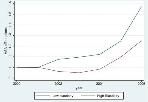
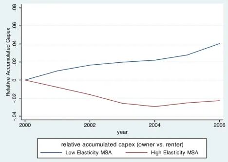
Figure 1 shows the evolution of office prices from 2000 to 2006 depending on the MSA local housing supply elasticity. It confirms that, while the bubble had a more dramatic impact on residential prices, it did also affect commercial prices. Low elasticity MSAs experienced a much larger increase in office prices (30% increase in 2 years) than high elasticity MSAs. Figure 2 implements our methodology looking at total capital expenditures since 2000, normalized by assets in 2000. In low elasticity MSAs, firms owning their headquarters experienced a 4 percentage points higher growth in capital expenditure (blue line) relative to firms renting their headquarters. By contrast, in high elasticities MSAs, there is no statistically significant difference in the evolution of assets of firms owning their headquarters relative to firms renting them (red line). If anything, owners saw a smaller increase in capital expenditure than renters (by about 2 percentage points). Figure 3 leads to similar conclusions on long-term debt: firms owning their headquarters in low elasticity MSAs took advantage of the real estate price bubble to increase their stock of debt relative to firms in similar MSAs but renting headquarters and relative to MSAs where the bubble did not have a large impact on office prices.
Table 10 confirms these graphical evidence using firm-level regressions. We adopt a standard long-run difference-in-difference strategy and estimate the following equation:
CAP EX00im−06 Assets00
im
=αm+β
∆(Of f ice P rice)00−06
m
Of f ice P rice00
m
×Headquartersi+γ
∆(Of f ice P rice)00−06
m Of f ice P rice00 m +im (5) where CAP EX 00−06 im
Assets00im is the sum, for firm i, of capital expenditures from 2000 to 2006, normalized
by 2000’s assets. ∆(Of f ice P rice)
00−06
m Of f ice P rices00
m is, for MSAm, the cumulative office price growth from 2000
to 2006. Finally,Headquartersi is a dummy equal to 1 if firm i owns its headquarters in 2000,
Column (1) in Table 10 directly estimates equation (5). The results from this dummy specification using the information from the 10K files are to be compared to Column (8) of Table 6. The .17 coefficient suggests that in response to a 10% real estate price increase, a firm that owns its headquarters will increase its investment rate by 1.7 percentage point more than a renting firm. The coefficient obtained through focusing on the 2000s is two times larger than our previous estimates (and than estimates of Gan, 2007a).
Column (2) replaces the local office price growth by the local housing supply elasticity: this corresponds to the reduced form of an instrumental variable regression where local prices are instrumented by local housing elasticity. As expected, since the higher the local housing elasticity, the lower the increase in local land prices, we find a negative sign on the interaction between housing elasticity and the owner dummy: in MSAs with a high housing elasticity, price increases have been moderate, and there is not much difference in the investment of owners compared to renters; in MSAs with a low housing elasticity, price increases have been dramatic, and owners increase their investment more than renters
Column (3) augments the previous regression in Column (2) by controlling for initial firm size. This is natural as there is a fair amount of heterogeneity between firms that own versus rent their headquarters.
Column (4) uses quartiles of local housing supply elasticity instead of the elasticity itself. Finally, Columns (5)-(8) replicate the regressions in Columns (1)-(4), replacing cumulative
investment by cumulative long term debt issues (∆Debt
00−06
im Assets00
im ) as the dependent variable.
Overall, the results in Table 10 confirm the analysis of Figures 2 and 3. Firms owning their headquarters experienced a significantly larger growth in assets and long-term debt relative to renters, especially so in MSAs where office prices increased a lot, i.e. in MSAs with lower housing supply elasticity. This effect is monotonic in the local housing supply elasticity.
4
Conclusion
When the value of a firm’s real estate appreciates by $1, its investment increases by approx-imately $.06. This investment is financed through additional debt issues. The impact of real estate shocks on investment is stronger when estimated on a group of firms which are more likely to be credit constrained. As we showed in this paper, real estate represents a significant fraction of the assets held on the balance sheet of corporations. As a consequence, one could expect the impact of real estate shocks on aggregate investment to be non-trivial. However, this is not necessarily the case in a world where responses to balance sheet shocks are heterogeneous. In particular, small firms respond more than large firms, which attenuates the aggregate impact of credit constraints. Understanding how one can go from the micro estimates we offer in this paper to the macro impact of real estate shocks on investment, and therefore on GDP, remains unclear. We hope to tackle this question in future research.
References
Almeida, Heitor, Murillo Campello and Michael S. Weisbach, 2004. “The Cash Flow Sensitivity
of Cash,” Journal of Finance, American Finance Association, 59(4):1777-1804.
Barro, Robert J, 1976. “The Loan Market, Collateral, and Rates of Interest,” Journal of
Money, Credit and Banking, Ohio State University Press, 8(4):439-56.
Benmelech, Efraim, Mark J. Garmaise and Tobias J. Moskowitz, 2005. “Do Liquidation Values Affect Financial Contracts? Evidence from Commercial Loan Contracts and Zoning
Regulation,” The Quarterly Journal of Economics, 120(3):1121-1154.
Benmelech, Efraim and Nittai Bergman, 2009. “Collateral Pricing”, Journal of Financial
Economics, 91(3) 339-360.
Benmelech, Efraim and Nittai Bergman, 2008. “Liquidation Values and the Credibility of
Fi-nancial Contract Renegotiation: Evidence from U.S. Airlines,” Quarterly Journal of Economics,
123(4): 1635-1677.
Bernanke, Benjamin and Mark Gertler, 1989. “Agency Costs, Net Worth and Business
Fluctuations” American Economic Review, 79(1):14-34.
Bernanke, Benjamin S, 1983. “Nonmonetary Effects of the Financial Crisis in Propagation
of the Great Depression,” American Economic Review, 73(3):257-76.
Bertrand, Marianne, Esther Duflo and Sendhil Mullainathan, 2004. “How Much Should We
Trust Difference in Difference Estimators ?”,Quarterly Journal of Economics, 119:249-275
Case, Karl, Quigley, John and Robert Shiller , 2001. “Comparing Wealth Effects: The Stock Market Versus the Housing Market,” NBER Working Paper N.8606.
Cutts, Robert, L., 1990. “Power from the Ground Up: Japan’s Land Bubble”, Harvard
Business Review, 68:164-72.
Eisfeldt, Andrea, and Adriano Rampini, 2009. “Leasing, Ability to Repossess, and Debt
Capacity,” Review of Financial Studies, Vol. 22, Issue 4, pp. 1621-1657.
Gan, Jie, 2007a. “Collateral, Debt Capacity, and Corporate Investment: Evidence from a
Natural Experiment”,Journal of Financial Economics, 85:709-734.
Gan, Jie, 2007b. “The Real Effects of Asset Market Bubbles: Loan- and Firm-Level Evidence
of a Lending Channel”,Review of Financial Studies, 20:1941-1973.
Goyal, Vidhan and Takeshi Yamada, 2001. “Asset Price Shocks, Financial Constraints and Investment: Evidence From Japan,”Journal of Business, 77(1):175-200
Hart, Oliver and John Moore, 1994. “A Theory of Debt Based on the Inalienability of Human
Capital,” The Quarterly Journal of Economics, 109(4):841-79.
Prices: Bubbles, Fundamentals and Misperceptions,” Journal of Economic Perspectives, 19(4):67-92.
Kaplan, Steven N. and Luigi Zingales, 1997. “Do Investment-Cash Flow Sensitivities provide
Useful Measures of Financing Constraints?”,The Quarterly Journal of Economics, 112: 169-215.
Kiyotaki, Nobuhiro and Moore, John, 1997. “Credit Cycles”, Journal of Political Economy,
105 (2): 211–248.
Mian, Atif and Amir Sufi, 2009. “House Prices, Home Equity-Based Borrowing, and the U.S. Household Leverage Crisis”, Working Paper.
Nelson, Theron R., Thomas Potter and Harold H. Wilde, 1999. “Real Estate Asset on
Corporate Balance Sheets,” Journal of Corporate Real Estate, 2(1):29-40.
Peek, Joe and Eric S. Rosengren, 2000. ”Collateral Damage: Effects of the Japanese Bank
Crisis on Real Activity in the United States,” American Economic Review, 90(1):30-45, March.
Rampini, Adriano, and S. Viswanathan, 2010. “Collateral, Risk Management, and the
Dis-tribution of Debt Capacity,” Journal of Finance, 65, 2293-2322..
Rauh, Joshua D., 2006. “Investment and Financing Constraints: Evidence from the Funding
of Corporate Pension Plans,” Journal of Finance, 61(1):33-71.
Saiz, Albert, 2010. “On Local Housing Supply Elasticity”,Quarterly Journal of Economics,
125 (3): 1253-1296.
Sufi, Amir, 2009, “Bank Lines of Credit in Corporate Finance: An Empirical Analysis”, Review of Financial Studies, 22(3), 1057-1088.
Stiglitz, Joseph E. and Andrew Weiss, 1981. “Credit Rationing in Markets with Imperfect
Information,” American Economic Review, 71(3):393-410.
Townsend, Robert M. , 1979. “Optimal Contracts and Competitive Markets with Costly
A
Figures and Tables
Figure 1: Relative Evolution of Office Prices (High vs. Low Elasticity MSA, 2000-2006)
.9 1 1. 1 1. 2 1. 3 1. 4 1. 5 1. 6 M SA of fi c e pric es 2000 2002 2004 2006 year
Low elasticity High Elasticity
Note: This figure shows the average office price index (normalized to 1 in 2000) for MSAs in the bottom quartile of land supply elasticity (“Low Elasticity MSA”) in blue and MSAs in the top quartile of land supply elasticity (“High Elasticity MSA”) in red.
Figure 2: Relative Evolution of Accumulated Capex (owners vs. renters, 2000-2006) -. 04 -. 02 0 .02 .04 .06 .08 R elat iv e Ac c um ulat ed C apex 2000 2002 2004 2006 year
Low Elasticity MSA High Elasticity MSA
relative accumulated capex (owner vs. renter)
Note: This figure shows, for each year between 2000 and 2006, the difference between the average accumulated capex of headquarter owners minus the average accumulated capex of headquarter renters, for MSAs in the bottom quartile of land supply elasticity (“Low Elasticity MSA”) in blue and MSAs in the top quartile of land supply elasticity (“High Elasticity MSA”) in red. Accumulated capex is defined as 0 in 2000, and then as the sum of all capex made by the firm between 2001 and the current year, normalized by assets in 2000.
Figure 3: Relative Evolution of Aggregate Debt (owners vs. renters, 2000-2006) -. 04 -. 02 0 .02 .04 .06 .08 R elat iv e D ebt Grow th 2000 2002 2004 2006 year
Low Elasticity MSA High Elasticity MSA relative debt growth (owner vs. renter)
Note: This figure shows, for each year between 2000 and 2006, the difference between total debt growth of headquarter owners minus total debt growth of headquarter renters, for MSAs in the bottom quartile of land supply elasticity (“Low Elasticity MSA”) in blue and MSAs in the top quartile of land supply elasticity (“High Elasticity MSA”) in red. Debt growth is defined as 0 in 2000, and then as the sum of all long term debt issued by the firm between 2001 and the current year, normalized by assets in 2000.