Automatic Security Protocol Analysis
Cas J.F. Cremers1⋆, Pascal Lafourcade2⋆⋆, and Philippe Nadeau3
1 Department of Computer Science, ETH Zurich, 8092 Zurich, Switzerland
2 Verimag, University of Grenoble, 38610 Gi´eres, France
3 Faculty of Mathematics of the University of Vienna, Austria
Abstract. There are several automatic tools available for the symbolic analysis of security protocols. The models underlying these tools differ in many aspects. Some of the differences have already been formally related to each other in the literature, such as difference in protocol execution models or definitions of security properties. However, there is an impor-tant difference between analysis tools that has not been investigated in depth before: the explored state space. Some tools explore all possible behaviors, whereas others explore strict subsets, often by using so-called scenarios.
We identify several types of state space explored by protocol analysis tools, and relate them to each other. We find previously unreported dif-ferences between the various approaches. Using combinatorial results, we determine the requirements for emulating one type of state space by combinations of another type.
We apply our study of state space relations in a performance compari-son of several well-known automatic tools for security protocol analysis. We model a set of protocols and their properties as homogeneously as possible for each tool. We analyze the performance of the tools over com-parable state spaces. This work enables us to effectively compare these automatic tools, i. e., using the same protocol description and explor-ing the same state space. We also propose some explanations for our experimental results, leading to a better understanding of the tools.
1
Introduction
Cryptographic protocols form an essential ingredient of current network nications. These protocols use cryptographic primitives to ensure secure commu-nications over insecure networks. The networks are insecure in two ways: attack-ers may analyze or influence network traffic, and communication partnattack-ers might be either dishonest or compromised by attackers. Despite the relatively small size of the protocols it is very difficult to design them correctly, and their analysis is complex. The canonical example is the famous Needham-Schroeder protocol [40], that was proven secure by using a formalism called BAN logic. Seventeen years
⋆Partially supported by the ComposeSec project (MANCOM).
later G. Lowe [33], found a flaw by using an automatic tool Casper/FDR. The flaw was not detected in the original proof because of different assumptions on the intruder model. However, the fact that this new attack had escaped the at-tention of the experts was an indication of the underestimation of the complexity of protocol analysis. This example has shown that automatic analysis is critical for assessing the security of such cryptographic protocols, because humans can not reasonably verify their correctness.
A few years later it was proven that the security problem is undecidable [1,28] even for restricted cases (see e. g. [20] for a survey). This undecidability is one of the major challenges for automatic analysis. For instance, in the tool used by Lowe, undecidability is addressed by restricting the type of protocol behaviors that were explored. The protocol that Lowe investigated has two roles. These roles may be performed any number of times, by an unbounded number of agents. Lowe used his tool to check a very specific setup, known as ascenario. Instead of exploring all possible protocol behaviors, the protocol model given to the tool considers a very small finite subset, in which there are only a few instances of each role. Furthermore, the initiator role is always performed by a different agent than the responder role. The attack that Lowe found exactly fits this scenario. However, if there would have been an attack that requires the intruder to exploit a large number of instances of the responder role, Lowe would not have found this particular attack with the tool. Addressing this problem, he provided a manual proof for the repaired version of the protocol, which states that if there exists any attack on that protocol, then there exists an attack within the scenario. Ideally, we would not need such manual proofs, and explore the full state space of the protocol automatically, or at least a significant portion of it.
Over the last two decades many automatic tools based on formal analysis techniques have been presented for the analysis of cryptographic protocols [2, 8, 11,12,19,22,35,37,39,43,44]. These tools address undecidability in different ways: either by restricting the protocol behaviors similar to the approach used by Lowe, or by using abstraction methods. However the restrictions put on the protocol behavior are rarely discussed or compared to the related work. Moreover, the tools provide very different mechanisms to restrict the protocol behaviors, and the relations between these mechanisms has not been investigated before.
This work started out as an investigation into the performance of protocol analysis tools. In contrast to the large number of tools, there are hardly any comparison studies between the different tools. In each tool paper the authors propose some tests about their tools’ efficiency, by describing the performance of the tool for a set of protocols. These tests implicitly use behavior restrictions, which are often not specified and sometimes are designed specifically to include known attacks on the tested protocols. Choosing different restrictions has a very clear impact on the accuracy as well as the performance of the analysis process. In particular, imposing stronger restrictions on the protocol behavior implies that fewer behaviors need to be explored, which means that for most tools the time needed for the analysis will be exponentially lower.
Contributions: In this paper we address two distinct, but very closely related problems. First, we discuss types of behavior restriction models used by protocol analysis tools, which we will also refer to as the exploredstate space. We show how these different state spaces are related to finding, or missing, attacks on protocols, and show how to match up certain state space types. Using math-ematical results, we compute the number of concrete scenarios that needs to be considered in order to analyze all the possible behaviors involving up to n
protocol role instances, or threads. Second, we use the knowledge gained about state spaces to perform a tool performance case study. We try to match up the exact restrictions used in each tool, and compare their performance on similar state spaces. We use our unfolding of symbolic scenarios to generate the input files for each tool in the test. This leads to new insights in the performance of the tools for secrecy and authentication properties.
Related work: To the best of our knowledge, the difference between state spaces in security protocol analysis has not been investigated before. However, some work exists on comparing the performance of different security protocol analysis tools. In [36] C. Meadows compares the approach used by NRL [37] and the one used by G. Lowe in FDR [42] on the Needham-Schroeder example [40]. She examines the difference and concludes that the two tools are complementary even though NRL was considerably slower. In [3], a large set of protocols is verified using the AVISS tool and timing results are given. In [47], a similar test is performed using the successor of AVISS, called the Avispa tool suite [2]. As the AVISS/Avispa tools consist of respectively three and four back end tools, these tests effectively work as a comparison between the back end tools. No conclusions about the relative results are drawn in these articles. A qualitative comparison between Avispa and Hermes [12] is presented in [30] and provides general advice for users of these tools. The comparison is not based on testing but on conceptual differences between the modeling approaches. In [15], a number of protocol analysis tools are compared with respect to their ability to find a particular set of attacks.
Outline: In Section 2 we describe and relate some of the different state spaces considered in symbolic protocol analysis. In Section 3 we determine the number of concrete scenarios needed to cover the same state space as a given symbolic scenario. In Section 4 we present our performance comparison experiments. We describe the choice of tools and test setup. We then discuss the results of the analysis before we move to the conclusions and future work in the last section.
2
State spaces in security protocol analysis
In the symbolic analysis of security protocol, one models both the agents that ex-ecute a security protocol, as well as the possible behavior of the active intruder. Combined these yield a system which should model (at some level of abstraction)
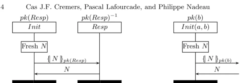
pk(Resp) Init pk(Resp)−1 Resp FreshN {|N|}pk(Resp) N
Fig. 1.An example protocolEX.
pk(b)
Init(a, b)
FreshN
{|N|}pk(b) N
Fig. 2. An example protocol instance
for the initiator role ofEX.
all possible behaviors of the agents in the presence of an active intruder. Veri-fying security properties of a protocol amounts to checking whether all possible behaviors of the resulting system satisfy the desired security property.
In such a model, agents may initiate a protocol or respond to incoming mes-sages. Consider the example protocolEX shown in Figure 1. There are two roles
Init (initiator) andResp (responder). An agenta can initiate a session of the protocol at some point by starting to execute the initiator role. He chooses who he wants to communicate with, for exampleb. Next he generates a fresh random numberN, and sendsN encrypted with the public keypk(b) of the agentb. After that he waits until he receives from the network the numberN back. The agent
b accepts incoming messages encrypted with its public key pk(b). Once such a message is received from an agent (for example, froma),bstarts an instance of the responder role. Following the model of the responder role,bwill accept and decrypt the message, and send back the resulting numberN to a.
In general, any number of agents may be running the protocol in parallel, and agents can also start multiple sessions with any other agent at the same time as responding to incoming messages.
2.1 Process model
We first give a high-level description of the protocol analysis problem in terms of processes. It is not our intent to go into full detail but only to provide the required knowledge for understanding the state space restrictions in the remainder of this paper. For further details we refer the reader to e. g. [21].
We recall some process calculus basics. Aprocess Pdefines a possibly infinite number of possible behaviors, where each possible behaviour is represented as a sequences of events. A possible sequence of events is referred to as atrace of the system. All possible behaviors of a process P are denoted by its set of traces, denoted by tr(P). We writeX kY to denote the process consisting of the parallel composition of the process X andY. We write !X to denote the replication of the processX, i.e. !X =X k (!X). We write + to denote the choice operator, which is generalized to P
for choosing over a parameter range.
A security protocol is defined as a finite set of communicating processes, referred to as “roles”. More precisely, we define a protocol as a mapping from
role names to processes. In practical applications, these roles have names such as client/server/. . ., or initiator/responder. A role usually consists of a sequence of send and receive events, and implicit or explicit generation of messages or fresh values such as nonces or session keys. In this paper we will not go into details of the allowed actions in a role.
Roles are executed by agents. Upon execution, any identifiers referring to role names in the protocol are instantiated with concrete agent names. For a protocol Qwith |dom(Q)| =n roles, where dom(Q) = {r1, . . . , rn}, we denote by Q(x)(a1, . . . , an) the process that is the instantiation of the role x, where
r1 is substituted by a1, etc.. This notation is effectively used as a shorthand for the more commonly used substitution notation Q(x)[a1, . . . , an/r1, . . . , rn]. For example, in Figure 2 we show the process EX(Init)(a, b). We allow some parameters to be unspecified, notation , which we interpret to be the unspecified choice between any of the possible agents from the set Agent. We will return later to exact the specification of the agent set, but remark here that a finite set will suffice for our purposes. In particular, we define for any protocolQthat
Q(x)(a1, . . . , , . . . , an) =
X
i∈Agent
Q(x)(a1, . . . , i, . . . , an).
Hence for the example protocol Q, Q(Resp)(, ) denotes a single execution of the responder role, with any choice for the agent names.
An agent can perform any role any number of times in parallel. Thus, for any protocolQ, the behavior of the agents is defined by the process
x∈dom(Q)!Q(x)( , . . . , ).
The messages are transmitted over a network that is considered to be insecure. It is insecure in the sense that an adversary or intruder can eavesdrop on any message, or insert his own messages. Furthermore, we assume an intruder may also have corrupted certain agents, for example because he has learnt their pri-vate keys, allowing him to impersonate the corrupted agents. Because agents may not know who has been corrupted, the non-corrupted agents may still start protocol sessions with corrupted agents.
This situation is commonly modeled by a single “intruder” who is represented by the process Intruder. The Intruder process can take messages from the network, manipulate them, insert messages into the network, or generate fresh values. Furthermore, the intruder has corrupted the agente, thereby learning its long-term secrets, including the long-term private keys of e.
Definition 1 (Sys). Given a protocolQ, the system describing the behavior of the agents in the context of the intruder is defined as
Sys(Q) =Intruderk
x∈dom(Q)!Q(x)(, . . . , ).
If there exists an attack on (a trace property of) a protocolQ, it is represented in the set of traces of the systemSys(Q). Conversely, if no trace in tr(Sys(Q)) exhibits an attack, there is no attack on the protocolQ.
2.2 Restricting the state space
Because of undecidability or efficiency concerns, protocol analysis tools usually apply some restrictions on the system and do not explore all elements from the set tr(Sys(Q)). More precisely, the system verified is not the full system Sys
described earlier, but rather a system which exhibits a subset of the behaviors of the full model. Such a subset can be defined by using aScenario.
AScenariois a multi-set of processes.Sdenotes the set of all possible scenar-ios and letScdenote the set ofconcrete scenarios in which no unspecified agents ( ) occur. We write {{a, a, b}} to denote the multi-set containing the elementa
twice, andbonce.
Definition 2 (Scen). Let S be a scenario. Then,
Scen(S) =Intruderk
p∈Sp.
In this paper we require that the processes in a scenarioS do not contain the replication operator. Observe that whereSys(Q) always contains an unbounded number of replications, Scen(S) contains only the intruder processes and the processes specified in S.
A generalization of theScensystem is the repeated scenario system.
Definition 3 (RepScen). RepScen(S)is defined for any scenario S as
RepScen(S) =Intruderk p∈S!p.
In contrast, a MaxRuns(Q, m) system is defined by a protocolQand a maximum count m. (The name derives from the term “run” referring to a role instance.) Where the systemSys(Q) contains any number of replications of each role, the MaxRuns system contains only a finite number of replications of each role.
Definition 4 (MaxRuns). Let Qbe a protocol, and letm be an non-negative integer. Then, MaxRuns(Q, m) =Intruderk m i=1( X x∈dom(Q) Q(x)(, . . . , )).
2.3 Relations between state space restrictions
Each restriction from the previous section effectively restricts the state space of the process model. We focus on trace-based security properties such as secrecy and authentication. Hence, when talking about correctness of a protocol, we refer to the full set of possible behavior histories (traces) of the system, denoted by tr(Sys(Q)). As we will see in Section 4, most tools do not explore this set.
LetQbe a protocol. For the set of all possible scenariosS, we have: ∀m∈N: tr(MaxRuns(Q, m))⊂tr(Sys(Q)) (1)
∀s∈ S: tr(Scen(s))⊂tr(Sys(Q)) (2) ∀s∈ S: tr(RepScen(s))⊆tr(Sys(Q)) (3) ∃s∈ S: tr(RepScen(s)) = tr(Sys(Q)) (4)
Proof. The relations (1),(2) and (3) above are immediate consequences of the definitions, as the left hand sides imply restrictions on the full set tr(Sys(Q)). For relation (4) we have that if the scenarios includes all possible process de-scriptions, the repetition of the processes inseffectively amounts to the full set of behaviors without any restrictions.
We write|s|to denote the number of elements of the scenarios. Relating the scenario-based approaches to the bounding of runs, we find:
∀s∈ S : tr(Scen(s))⊆tr(MaxRuns(Q,|s|)) (5) Observe that if the scenario contains |s| runs, the resulting traces will never contain more, and thus this included in MaxRuns(Q,|s|).
The next formula expresses that there exist no concrete scenarios that cor-respond exactly to a MaxRuns trace set.
∀n∈N+:∀s∈ Sc: tr(Scen(s))6= tr(MaxRuns(Q, n)) (6)
Proof. For any n > 0, tr(MaxRuns(Q, n)) contains a trace with n role pro-cesses. In particular, it will also contain a trace containing n instances of the first role, and also a trace containing n instances of the second role. To match tr(MaxRuns(Q, n)) to tr(Scen(s)),smust also contain exactlynrole processes. Because we are considering only concrete scenarios, we need to define ins the first case (ntimes the first role). However, by this definition ofswe have excluded the second type of traces with only the second role.
Assuming a finite number of agents, ∀n∈N,∃k:∃s1, . . . , sk ∈ Sc:
k
[
i=1
tr(Scen(si)) = tr(MaxRuns(Q, n)) (7) The last formula expresses that for a finite set of agents, we can enumerate all possible scenario descriptions of n role processes, and turn them into scenario sets. The result of this formula is that we can match up the trace sets of MaxRuns and Scen by unfolding. This opens up a way to make the state spaces uniform.
3
Generation of uniform state spaces
Starting from a state space described using MaxRuns(Q, n) for an integern, we generate a set of concrete scenarios that exactly covers the same state space, by using Formula (7). Further parameters involved in the generation of this set of scenarios are the number of roles of the protocol and the number of agents.
3.1 Required number of agents
In protocol analysis it is common to use two honest agents and a single untrusted (compromised) agent. The underlying intuitions are that the security properties
under consideration are invariant under renaming of the (honest) agents, and that a single intruder is as strong as multiple colluding intruders. In general, attacks might require more agents, depending on the protocol under investigation and the exact property one wants to verify. A number of results related to this can be found with proofs in [17]. We recall the results of this paper as we will use them in the context of this paper.
– Only a single dishonest (compromised) agente, needs to be considered for the analysis of the class of properties under consideration here.
– For the analysis of secrecy, only a single honest agentais sufficient.
– For the analysis of authentication for protocols with two roles, we only need two honest agentsaandb.
For example, for a single honest agentaand a single compromised agent e, for a protocol with roles{r1, r2}, tr(MaxRuns(Q,1)) is equal to
[
k∈{a,e}
tr(Scen({{r1(a, k)}})) ∪ [ k∈{a,e}
tr(Scen({{r2(k, a)}})),
which yields a set of four scenarios.
3.2 Computing the number of concrete scenarios
For a given integer n, we can derive the size of a set M of concrete scenarios, such thatS
s∈Mtr(s) = tr(MaxRuns(Q, n)). This size ofM corresponds to the value ofkin Formula (7) under the assumption of a finite number of agents and trace equivalence under renaming.
For a single agent (involved in the verification of secrecy), the generation of a set of concrete scenarios is a trivial application of the binomial coefficient. For two agents or more the situation is not so simple, because the generation of the set is complicated by the fact that scenarios are considered equivalent up to renaming of the honest agents.
Example 1 (Renaming equivalence). LetP be a protocol with a single roler1. Consider the state space MaxRuns(Q,2) for two honest agentsa, b. Consider the following scenario set:
{{r1(a), r1(a)}}, {{r1(a), r1(b)}}, {{r1(b), r1(b)}}
Because the names of the honest agents are interchangeable, the last scenario is equivalent up to renaming to the first one. In order to verify security properties, we would need only to consider the first two scenarios.
We generalize this approach by considering|R|roles in the protocol description. We assume that we have two agents a and b and one intruder. Let n be the parameter of MaxRuns(Q, n) for which we want to generate the equivalent set of scenarios. In order to choose a run description X(a1, . . . , a|R|), we have |R|
the attacker for eacha2, . . . , a|R|, and we find there are 2∗ |R| ∗3(|R|−1)different
possible run descriptions. Now we have to choose a multi-set ofnrun descriptions among this set of all possible runs descriptions. We use the following formula:
2∗ |R| ∗3(|R|−1)+n−1
n
However, this does not take into account that scenarios are equal up to the re-naming of the (honest) agents. For example, we observe that{{r1(a, b), r2(b, a)}} is equivalent to{{r1(b, a), r2(a, b)}}under the renaming{a→b, b→a}.
We now use group theory results to compute the number of scenarios needed. We first consider the case with two agents and use Burnside’s lemma [13] then for the other cases we need to consider Polya’s Theorem which is a generalization of Burnside’s Lemma. In the rest of this section, we detail the case for two agents using Burnside and Polya then we present the case of three agents with Polya to give a flavor of the general case by this method.
3.3 Theoretical result for two agents
We recall that nk
= k!(nn−!k)! and Burnside’s lemma [13].
Lemma 1 (Burnside’s lemma).LetGbe a finite group that acts on a setX. For eachg inGletXg denote the set of elements inX that are fixed byg. Then
the number of orbits, denoted |X/G|, is:
|X/G|= 1 |G|
X
g∈G |Xg|
where|X| denotes the cardinality of the setX.
Thus the number of orbits (a natural number or infinity) is equal to the average number of points fixed by an element of G (which consequently is also a natural number or infinity). A simple proof of this lemma was proposed by Bogard [9].
We have to consider all the renamings and compute the number of scenarios that are stable by this operation. Because we have only two agents, we have only two possible renamings:
1. σId={a→a, b→b} (the trivial renaming) 2. σ1={a→b, b→a}
Observe first that|G|= 2 because we have two renamings. In the first case, all elements are fixed so we have 2∗|R|3(|Rn|−1)+n−1
possibilities. In the second case, the fixed elements are multi-sets of the sizenwhere the terms are associated by two and of their arguments are of the forma, x1, . . . , x|R|−1or b, x1, . . . , x|R|−1. It corresponds to choosing a multi-set of n
2 elements in a set where the first parameter is fixed, i. e., in a set of cardinality|R| ∗3(|R|−1). Notice that ifn is odd the second set is empty because in this case there is no way to get a fixed element using the second renaming.
Lemma 1 leads to the following formula, where ǫn is 0 if n is odd and 1 otherwise.k(n,|R|) is the number of scenariosk for Formula (7).
k(n,|R|) = 2∗|R|∗3(|R|−1)+n−1 n +ǫn |R|∗3 (|R|−1) +n 2−1 n 2 2 (8)
For instance for a protocol with |R| = 2 roles, the set of traces of the process MaxRuns(Q,2) is equal to the union of the trace sets defined byk(2,2) = 42 dif-ferent scenarios.1Note that if we would not have taken the renaming equivalence into account, we would instead generate 2∗2∗32−12 +2−1
= 78 scenarios.
3.4 Generalization using Polya’s Theorem
We first explain the theory needed for the application of Polya’s Theorem in our context. We then sketch the case of two agents (we obtain of course the same result as when using Burnside’s Lemma), after which we present the case of three agents to provide intuition for the general case of |A|agents.
Theory We note PP(R, A) the set R×A×(A∪ {e})|R|−1, where e is the compromised agent. For a givenn, letMPP(R, A, n) be the multi-sets of sizenof elements ofPP(R, A). We wish to compute the numberk(n,|R|), the number of orbits ofMPP(R, A, n) under the action of renaming the agents. We managed to solve this question directly in the case of two agents with the help of Burnside’s theorem, but for a general A there is no direct way to know how many fixed points a given renaming has on MPP(R, A, n). Hence we use Polya’s theorem, which leads to a more complicated but automatic way of computing k(n,|R|).
For σ a permutation of a set, we denote by ci(σ) the number of cycles of lengthi(the length of a cycle is the minimal number of applications of the cycle to get the identity back).
Suppose we have setsD(of finite cardinality|D|=d) andE, withGa group of permutations acting onD. LetED be the set of functions fromD to E. We say thatf, g∈ED are equivalent if there existsσ∈Gsuch thatf(σ(d)) =g(d) for alld∈D, and we noteF a set of representatives of the equivalence classes. Now letw be a function from E to a certain commutative ring k, and let the weight off ∈ED be W(f) :=Q
d∈Dw(f(d)). One notes easily that iff andg are equivalent, then W(f) = W(g). We define W(F) = P
f∈FW(f), and the
cycle indicator polynomial PG(x1, . . . , xd) = |G1|Pσxc11(g)x c2(g)
2 . . . x cd(g) t . Then we can statePolya’s theorem[18, p.252]:
W(F) =PG X y∈E w(y),X y∈E w(y)2, . . . ,X y∈E w(y)d (9)
Let us now consider the application in our context. Ifσ is a renaming (i.e. a permutation of A), we define φ(σ) as the permutation that is induced on
PP(R, A), which is φ(σ)(ri(a1, . . . , a|R|)) :=ri(σ(a1), . . . , σ(a|R|)). In our case,
D is the set PP(R, A), on which the group of permutationsG={φ(σ)} acts, andEis the setNof nonnegative integers. Then, a multisetm∈MPP(R, A, n) is equivalent to a function f ∈ ED with P
df(d) = n: the integer f(d) is the number of occurrences ofdin the multiset. Note that two multisets are equivalent up to renaming precisely when the corresponding functions f, g are equivalent in the sense of Polya’s theorem.
Letk be the ring of power series in the variable q, and define w : E → k
by w(i) =qi; iff ∈ED is a multiset of size n, we getW(f) =Q
dw(f(d)) =
qP
df(d) = qn. From this we deduce easily that W(F) = P
nk(n,|R|)qn. We notice also that P
y∈Ew(y)i =
P
j∈Nq
ij = 1
1−qi. Then Polya’s theorem (9), in our context, says that if we perform the substitutions xi := 1−1qi in PG for all variablesxi, and expand the result in terms of powers ofq, the coefficient ofqn is exactlyk(n,|R|). Let us explicit the cycle indicator polynomial here:
P = 1 |A|! X σ xc1(φ(σ)) 1 x c2(φ(σ)) 2 . . . x ct(φ(σ)) t , (10)
We finally need to a way to compute the integers ci(φ(σ)), which is what the following formulas achieve
ci(φ(σ)) =1 i X d|i µ(i d)c1(φ(σ d)) fori >1 (11) c1(φ(σd)) =|R| ·( X i|d ici(σ))·(X i|d ici(σ) + 1)|R|−1 (12)
The first one can be found for instance in [32, p.95] (it is an instance of the
M¨obius inversion formula), the second one is an easy counting of the fixed points of φ(σd). We recall that the M¨obius function µ(n) is defined for all positive integersnas follows:µ(n) = (−1)k ifnis the product ofkdistinct primes, and
µ(n) = 0 otherwise.
We are now able to express concretely the polynomialP for any number of agents. We remind the reader of the following results for computing with power series: +∞ X n=0 anqn ! · +∞ X n=0 bnqn ! = +∞ X n=0 n X i=0 aibn−i ! qn 1 1−q i = ∞ X j=0 i+j−1 j qi
We will explicit the result for the case of 2 agents, and sketch the case for 3 agents to get an explicit formula.
Two agents Consider now the case of 2 agents aandb, so that we have only two renamings:σId ={a→a, b→b}andσ1={a→b, b→a}.
We first compute the polynomialP of Equation (10): using the formulas for theck(φ(σ)), we havec1(φ(σId)) =|R| ·2·3|R|−1,c2(φ(σId)) = 0,c1(φ(σ1)) = 0, andc2(φ(σ1)) =|R| ·3|R|−1. Hence, if we substitutex1:=1−1q1 andx2:= 1−1q2,
we obtain: P= 1 2(x 2·|R|·3|R|−1 1 +x |R|·3|R|−1 2 ) = 1 2( P∞ i=0 2·|R|·3|R|−1+i−1 i qi+P∞ i=0 |R|·3|R|−1+i−1 i q2j)
Now k(n,|R|) is given by the coefficient ofqn in this expression, so we have to distinguish the cases neven and nodd, and we find indeed the same result as with Burnside’s Lemma.
Three agents For three agentsa, bandc, we have|PP(R, A)|= 3· |R| ·4|R|−1. There are 3! = 6 renamings, and for each of them we have to compute the corresponding term in P. For instance, if we take σ1 ={a→b, b→a, c→c}, we havec1(φ(σ1)) =|R| ·2|R|−1,c2(φ(σ1)) = (|R| ·3·4|R|−1− |R| ·2|R|−1)/2 and
c3(φ(σ1)) = 0, which gives the corresponding term inP. Proceeding in the same way for all other renamings, we get
P = 1 6(x 3|R|·4|R|−1 1 + 3x |R|·2|R|−1 1 x (3|R|·4|R|−1−|R|·2|R|−1)/2 2 + 2x |R|·4(|R|−1) 3 )
We now substitute xi = 1−1qi for i = 1,2,3, and then take the coefficient of qn to obtain the value of k(n,|R|); this is easily done by the rules for com-puting with power series given above, and the result is the following: let αn :=
3|R|·4|R|−1+n−1 n , βn :=P [n 2] l=0 (3|R|·4|R|−1−|R|·2|R|−1)/2+l−1 l · |R|·2|R|−1n−+2ln−2l−1 , where [n
2] denotes the integer part of n/2), and γ3i =
|R|·4|R|−1+i−1
i
, while
γn= 0 if 3 does not dividen. Then we get the following result for three agents
k(n,|R|) = 1
6(αn+ 3βn+ 2γn)
The formula fork(n,|R|) can be constructed similarly for any number of agents.
3.5 Practical implications
In general, tools can explore radically different state spaces. With protocol anal-ysis, we are looking for two possible results: finding attacks on a protocol or having some assurance of the correctness of the protocol. If an attack on a pro-tocol is found, any unexplored parts of the state space are often considered of little interest. However, if one is trying to establish a level of assurance for the correctness of a protocol, the explored state space becomes of prime importance. As established in the previous section, even for two honest agents, the simplest protocols already need 42 concrete scenarios to explore exactly all attacks in-volving two runs.
In many cases, protocol models increase the coverage of small attacks (i. e. involving few runs) by including a scenario with a high number of runs. This process is error prone: as an example we mention that in the Avispa modeling [5] of the TLS protocol [41] a large scenario is used in the example files, which covers many small attacks, but not scenarios in which an agent can communicate with itself. As a result, the protocol is deemed correct by the Avispa tools, whereas other tools find an attack. This is a direct result of the fact that the used scenario does not cover all attacks for even a small number of runs. One can discuss the feasibility of such an attack, and argue that an agent would not start a session with herself, but the fact remains that the protocol specification does not exclude this behavior, and therefore certainly means that the protocol does not meet the security properties for its specification.
When one uses a tool for the analysis of a protocol one should be aware of the impact the state space choices have on the result of the analysis, in order to avoid getting a false sense of security from a tool.
4
Experiments
In this section we use the state space analysis of Section 2 to perform a com-parison between several tools on a set of well-known cryptographic protocols considering the same state space. In our experiments we automatically generate the necessary concrete scenarios according to the results obtained in Section 3. We first discuss some of the choices made for these experiments, after which we give the results of the tests.
4.1 Settings
Tool selection and method of comparison We compared tools that are freely available for download and for which a Linux command-line version exists. Consequently, we had to exclude some tools, e. g., we do not consider Athena [44] or NRL [37] as these tools are not available, and we do not consider Hermes [12] because its current version only has a web interface, making it unsuitable for performance comparisons. The tools we compare are the following:
Avispa (Version: 1.1 for Automated Validation of Iternet Security Protocols and Applications consists of the following four tools that take the same input language called HLPSL [2]:
· CL-Atse: (Version: 2.2-5) Constraint-Logic-based Attack Searcher applies con-straint solving with simplification heuristics and redundancy elimination techniques [46].
· OFMC: (Version of 2006/02/13) The On-the-Fly Model-Checker employs sym-bolic techniques to perform protocol falsification as well as bounded analy-sis, by exploring the state space in a demand-driven way. OFMCimplements a number of optimizations, including constraint reduction, which can be viewed as a form of partial order reduction [6].
· Sat-MC: (Version: 2.1, 3 April 2006) The SAT-based Model-Checker builds a propositional formula encoding all the possible traces (of bounded length) on the protocol and uses a SAT solver [4] (notice that you can modify some parameters and in particular the choice of the SAT solver in the configuration file of Sat-MC, we use the default configuration in our experiments). · TA4SP: (Version of Avispa 1.1) Tree Automata based on Automatic
Approx-imations for the Analysis of Security Protocols approximates the intruder knowledge by using regular tree languages and rewriting to produce under-and overapproximations [10].
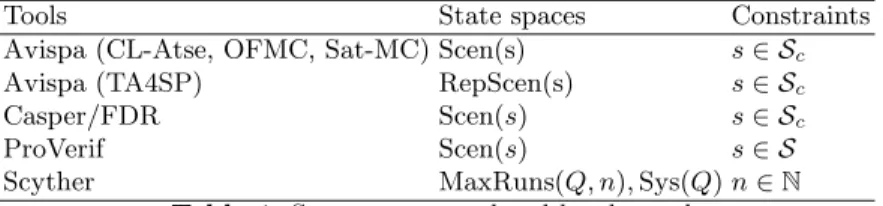
The first three Avispa tools (CL-Atse, OFMC and Sat-MC) take a concrete scenario (as required by the HLPSL language) and consider all traces of Scen(s). The last Avispa back-end, TA4SP, also takes a HLPSL scenario, but verifies the state space that considers any number of repetitions of the runs defined in the scenario, yielding RepScen(s). TA4SP is based on overapproximations and hence might find false attacks. As no trace is ever reconstructed by TA4SP, the user has no indication of whether the output “attack” corresponds to a false or true attack. Furthermore, there is a “level” parameter that influences whether just to use the overapproximation (level = 0), or underapproximations of the overapproximation (level>0). In the Avispa default setting only level 0 is explored by default, which in our test cases would have resulted in never finding any attacks, finding in 57% of all cases “inconclusive”, and in the remaining 43% “correct”. For our tests, we start at level 0 and increase the level parameter until it yields a result that is not “inconclusive”, or until we hit the time bound. This usage pattern is suggested both by the authors in [10] as well as by the output given by the back-end when used from the Avispa tool.
ProVerif: (Version: 1.13pl8) analyzes an unbounded number of runs by using over-approximation and represents protocols by Horn clauses. ProVerif [8] ac-cepts two kind of input files: Horn clauses and a subset of the Pi-calculus. For uniformity with the other tools we choose to model protocols in the Pi-calculus, which is closer than HLPSL (Avispa input language) than Horn clauses. ProVerif takes a description of a set of processes, where each defined processes can be started any number of times. The tool uses an abstraction of fresh nonce genera-tion, enabling it performs unbounded verification for a class of protocols. Given a protocol description, one of four things can happen. First, the tool can report that the property is false, and will yield an attack trace. Second, the property can be proven correct. Third, the tool reports that the property cannot be proved, for example when a false attack is found. Fourth, the tool might not terminate. It is possible to describe protocols in such a way that RepScen(s) is correctly modeled, resulting in the exploration of Sys(Q).
Scyther: (Version: 1.0-beta6) verifies bounded and unbounded number of runs, using a symbolic backwards search based on patterns [22, 23]. Scyther does not require the input of scenarios. It explores Sys(Q) or MaxRuns(Q, n): in the first case, even for smalln, it can often draw conclusions for Sys(Q). In the second
Tools State spaces Constraints
Avispa (CL-Atse, OFMC, Sat-MC) Scen(s) s∈ Sc
Avispa (TA4SP) RepScen(s) s∈ Sc
Casper/FDR Scen(s) s∈ Sc
ProVerif Scen(s) s∈ S
Scyther MaxRuns(Q, n),Sys(Q)n∈N
Table 1.State spaces explored by the tools
case, termination is not guaranteed. By default Scyther explores MaxRuns(Q,5), is guaranteed to terminate, and one of the following three situations can occur. First, the tool can establish that the property holds for MaxRuns(Q,5) (but not necessarily for Sys(Q)). Second, the property is false, yielding a counterexample. Third, the property can be proven correct for Sys(Q).
Casper/FDR: (Version: Casper 1.11 alpha-release, FDR 2.83) [35, 43] This tool uses consists of the Casper tool, which translates protocol descriptions into the process algebra CSP [29], and the CSP model checker FDR [42]. [27] provides a time based analysis of using the tool for analyzing a large collection of existing protocols. Lowe used Casper/FDR to find the man-in-the-middle attack on the Needham-Schroeder protocol [33].
A summary of the tools and their respective state spaces is given in Table 1.2In order to compare the tools fairly, we match up the state spaces. As a candidate for a common state space, any unbounded set (Sys(Q),RepScen) is not suitable. Furthermore, as Scen can be used to simulate MaxRuns, but not the other way around, we choose MaxRuns as the common denominator of the selected tools. We automatically generate for each number of runsn the corresponding input files to perform a fair time comparison over MaxRuns(Q, n). Note that the time measurements for the tools only include their actual running times, and does not include the time needed for the generation of the input files.
Security properties We consider the analysis of secrecy as well as authenti-cation. Secrecy can be modeled in each of the tools considered. Authentication cannot be modeled by TA4SP. The tools provide support for various security properties, ranging from several forms of agreement [34] to synchronization [25], or equivalence-based properties (ProVerif).
Protocol test set We consider a number of well-known protocols found in the literature [5, 14, 16, 31]. We select a set that can be modeled in all tools, which excludes protocols that use e.g. algebraic properties. We have restricted ourselves to the following four protocols: the famous Needham-Schroeder [40] using public
2 Note that the constraint for the Avispa tools is partly driven by its input language
HLPSL. For example, OFMC is able to analyzes∈ Sby modeling protocols in the
keys, and the corrected version by Lowe [33], EKE [7] which uses symmetric and asymmetric encryption, and finally TLS [41] as an example of a larger protocol.
Final setup details With respect to the analysis of multiple properties, we remark that some tools can test multiple properties at once, some cannot, and some stop the analysis at the first property for which an attack is found. We choose to analyze one security property at a time.
Guided by our results of the previous section, we automatically construct input files for the right scenarios for each protocol and for each tool. This in-volves the generation of all concrete scenarios to match the state space of a given number of runs. To this end we generate all scenarios (ignoring renaming equivalence) in the first phase, and filter out scenarios that are equivalent under renaming in the second phase. The number of generated scenarios is identical to the theoretical number computed in the previous section.
Our tests can be reproduced: all used scripts and models are downloadable from [24], and we have only used freely downloadable tools and well-known protocols. The tests have been performed using an Intel Core Duo processor, 2.0 GHz, with 1GB of ram using the Linux operating system.
4.2 Results
We use each tool to verify security properties of the selected protocols. In the first set of results we present the total analysis time, which corresponds to the total time needed for verifying all the properties of each protocol, for each tool. When a tool reaches the time limit, no conclusion can be drawn about the analysis time and hence no points (and connecting lines) are displayed for such cases. For a better visualization of the exponential behavior of some of the tools, we use a logarithmic scale.
We start our discussion of the results by presenting and analyzing the tests for secrecy for all tools. Afterwards we continue with the results for authentication for all tools which can deal with this property. Finally, we show a table which summarizes the unbounded verification performance for the tools which are able to deal with an unbounded number of runs, and the attack discovery performance for all tools.
Secrecy time results In Figure 3, we show the analysis time for the secrecy properties of the Needham-Schroeder-Lowe protocol (NSL3) as a function of the number of runsnof the state space explored, that is, MaxRuns(NSL3, n).
We observe that (as expected from the underlying models) ProVerif and TA4SP follow a constant time. Surprisingly Scyther has the same curve as ProVerif (close to the x-axis). Sat-MC, OFMC and CL-Atse follow an exponen-tial curve, where in this case CL-Atse is faster than OFMC. One other interesting point is that the curves of OFMC and Casper/FDR cross the Sat-MC curve: in other words, for larger numbers of runs, Sat-MC is more efficient. This result is confirmed by the results for the EKE protocol, which we show below. One final
0.1 1 10 100 1000 1 2 3 4 5
Needham-Schroeder-Lowe : secrecy of na and nb for A,B
time (s) number of runs Casper/FDR CL-Atse OFMC ProVerif Sat-MC Scyther TA4SP
Fig. 3.Time efficiency comparison for Needham-Schroeder-Lowe [33], for secrecy
0.1 1 10 100 1000 timeout 1 2 3 4 5 6
EKE : secrecy of k for A,B
time (s) number of runs Casper/FDR CL-Atse OFMC ProVerif Sat-MC Scyther TA4SP
Fig. 4.Time efficiency comparison for EKE [7], secrecy
point to mention is that Scyther and ProVerif both show time performances of less than one second for all the security properties considered for this protocol. We also remark that Casper/FDR has an exponential curve and is slower than OFMC and CL-Atse, but faster than Sat-MC for a small number of runs.
In Figure 4, we present the efficiency results for the EKE protocol [7]. This protocol shows again that the bounded analysis tools (Sat-MC,OFMC,CL-Atse) follow an exponential curve, as well as the hybrid Scyther, which has for this particular protocol also an exponential curve, albeit with much lower times than the other bounded tools. We also observe that Sat-MC has a slower exponential curve than OFMC and CL-Atse. ProVerif is still constant (here fluctuations are due to millisecond noise during testing). We also notice that TA4SP has a constant analysis time but with an high time computation even for one process. This is due to the modeling of the protocol and to the fact that TA4SP has to construct in all cases of this protocol a complex tree automaton to perform its
0.1 1 10 100 1000 timeout 1 2 3 4 5 6
TLS : secrecy of ck and sk for A,B
time (s) number of runs CL-Atse OFMC ProVerif Sat-MC Scyther TA4SP
Fig. 5.Time efficiency comparison for TLS [41], secrecy
analysis. For this protocol, Casper/FDR already exceeds the time limit for the smallest state space.
The last protocol analyzed with respect to secrecy is presented in Figure 5. TLS [41] is a relatively complex protocol, and certainly the most complex proto-col in this small test set. Hence, we expected the tools to spend some effort and time to get to a result. Our hypothesis was confirmed, as e.g. Sat-MC reaches the time limit for a fairly small state space. In this example, as in the previous one (EKE), we can also see the difference between OFMC and CL-Atse, where in this example CL-Atse is faster that OFMC. This protocol also confirms the results of Scyther which remains competitive with ProVerif and TA4SP. These three tools have all very fast time results and the variations on the curves are very small (less than 0.1 second).
Authentication time results In this section we present the results for the tools which can deal with authentication properties of the selected protocols.
In Figure 6, we analyze the performance of for authentication properties of the Needham-Schroeder protocol. ProVerif and Scyther are faster than the other tools used (results close zero second). Casper/FDR, CL-Atse and OFMC are very close and follow an exponential curve, with a minor advantage for Casper/FDR for a small number of runs.
In Figure 7, we see that the tools stop after having found an attack, which explains the flat shape for CL-Atse. In case of OFMC, there is still an exponential curve although an attack is found. We conjecture that this is caused by the specifics of the partial order reduction scheme, which effectively work like a heuristic: sometimes a non-optimal choice is made, causing the tool to explore a larger part of state space before the attack is found. The same explanation is valid for the smooth increasing of the Sat-MC curve towards the time limit. In this case Scyther is the fastest tool. ProVerif has constant time and is slower than all others for a small number of runs for this property of EKE.
0.1 1 10 100 1000 timeout 1 2 3 4 5 6
Needham-Schroeder : authentication of A,B
time (s) number of runs Casper/FDR CL-Atse OFMC ProVerif Sat-MC Scyther
Fig. 6.Time efficiency comparison for Needham-Schroeder [40], authentication
0.1 1 10 100 1000 timeout 1 2 3 4 5 6
EKE : authentication of A,B
time (s) number of runs Casper/FDR CL-Atse OFMC ProVerif Sat-MC Scyther
Fig. 7.Time efficiency comparison for EKE [7], for authentication
In Figure 8, we observe that Scyther is the most efficient with times of less than one second. For TLS we have that Sat-MC reaches the time limit for the two authentication claims when analyzed for one run, but quickly finds a flaw for state spaces with least two runs. For OFMC and CL-Atse we again observe very similar time results.
5
Results and discussion
We summarize the efficiency of finding attacks on the secrecy properties of the Needham-Schroeder protocol in Table 2. Next, we present a verification compar-ison for the tools capable of unbounded verification in Table 3. Finally we draw conclusions from our performance analysis.
0.1 1 10 100 1000 timeout 1 2 3 4 5 TLS : authentication of A,B time (s) number of runs CL-Atse OFMC Sat-MC Scyther
Fig. 8.Time efficiency comparison for TLS [41], for authentication
Secrecy CL-Atse Casper/FDR OFMC ProVerif Sat-MC Scyther TA4SP
A na no att no att no att no att no att no att no att
A nb no att no att no att 0.00 (1!) no att no att 1.44 (1?)
B na 0.18 (2!) 0.65 (2!) 0.25 (2!) 0.00 (1!) 2.36 (2!) 0.00 (2!) 0.47 (1?)
B nb 0.25 (2!) 0.47 (2!) 0.24 (2!) 0.00 (1!) 2.34 (2!) 0.00 (2!) 0.47 (1?)
Table 2.Finding an attack on Needham-Schroeder for secrecy
Comparison of attack finding efficiency We first introduce the notation used in the Table 2: “no att” means the tool finds no attack, 0.12(2!) means that the tool finds an attack in 0.12 seconds with two processes, and 0.13(1?) means that the tool finds an attack in 0.13 seconds with two processes, but it might represent a false attack.
First we notice that ProVerif finds an attack on roleA for the nonceN b. If we use Scyther with the specific option (–untyped), the existence of the attack is confirmed. As we use the tools with their default setting, it is expected that some tools do not find this flaw. Unfortunately we have no way of knowing what the attack found by TA4SP looks like. This is an interesting result, because according to the specification of this tool it used a typed model as dictated by the HLPSL input specification, so the type flaw attack should not occur, and we would expect TA4SP not to find an attack. However, as we have no way to extract the TA4SP “attack” we assume it is a false attack in this case.
Second we can see that with our modeling, and using the results from [17] which state that considering one honest agent is sufficient for the analysis of secrecy, ProVerif can quickly find attacks. All the other tools need two runs to find the man-in-the middle attack, as expected.
Finally we find again our conclusion regarding efficiency that Scyther and ProVerif are the fastest, then TA4SP (but the status of the attacks remains unconfirmed), then CL-Atse and OFMC are second with a very small advantage
Secrecy ProVerif Scyther TA4SP EKE A k 0.07 (1) - 11.16 (1) B k 0.12 (1) - 11.20 (1) Needham-Schroeder A na 0.00 (1) 0.00 (3) 1.92 (1) A nb attack! 0.00 (3) attack?
B na attack! attack! attack?
B nb attack! attack! attack?
Needham-Schroeder-Lowe A na 0.00 (1) 0.00 (3) 1.70 (1) A nb 0.00 (1) 0.00 (3) 1.85 (1) B na 0.00 (1) 0.00 (4) attack? B nb 0.00 (1) 0.00 (3) 1.71 (1) TLS A ck 0.02 (1) 0.07 (2) inconclusive A sk 0.01 (1) 0.06 (2) inconclusive B ck 0.02 (1) 0.04 (2) inconclusive B sk 0.02 (1) 0.06 (2) inconclusive
Table 3.Performance of unbounded verification
to CL-Atse (which has been confirmed in the previous analysis with more runs), then Casper/FDR and finally Sat-MC.
Comparison of unbounded verification performance In this part we an-alyze the performance of tools which are able to prove the correctness of a protocol. This includes Scyther, ProVerif and TA4SP, where we have considered only the secrecy properties. We perform this analysis on the four selected pro-tocols, and detail the results in Table 3. With respect to the used notation, we mention that 0.12(3!) denotes the fact that the tool proves the correctness of the protocol with 3 runs in 0.12 seconds,attack? means that the tool claims to find an attack (but which we could not check),−means that there is no answer for our testing, inconclusive is only for TA4SP, indicating that the tool does not state anything about the property. For TLS, TA4SP was not able to provide any answers. For EKE, Scyther could not establish unbounded verification, and provided bounded analysis for MaxRuns(Q,7).
Time performance analysis conclusions This time performance analysis shows that overall, the fastest tool is ProVerif, then Scyther, TA4SP, CL-Atse, OFMC, Casper/FDR and finally Sat-MC.
ProVerif. ProVerif shows the fastest performance. The abstraction of nonces allows the tool to obtain an efficient verification result quickly for an unbounded number of runs. The results for EKE in Figure 4 indicate that ProVerif does not support equational theories very well. In this case the resolution generates much more Horn clauses than in the case without equational theory. To confirm the efficiency of ProVerif, we performed a comparison with Scyther for thefngn family of protocols from [38]. Members of this family are generated by an integer
parameter, corresponding to the number of instances required for an attack on the protocol. As a result, the complexity of verifying the protocol is related to this parameter. For this protocol, the time results for ProVerif increase, but are lower than the ones for Scyther.
Scyther. Scyther outperforms the other bounded tools and can often achieve the same performance as tools based on abstraction methods. For some protocols, no full verification can be performed, and the tool exhibits exponential verification time with respect to the number of runs.
OFMC/CL-Atse. The behaviors of OFMC and CL-Atse are mostly similar for the tested protocols. We observe that the curves produced by these two tools are exponential, which confirms the theoretical results for their underlying algo-rithms. Finally we observe that for the tested protocols, CL-Atse is somewhat faster than OFMC for higher numbers of runs.
Casper/FDR. Casper/FDR exhibits, for all examples that we tried, exponential behavior. In general, the analysis is slower than CL-Atse and OFMC.
Sat-MC. Sat-MC also has an exponential behavior and is slower than CL-Atse and OFMC for lower numbers of runs. In particular, Sat-MC has proven to be especially slow for the more complex protocol TLS. In contrast, for the smaller protocols we found that Sat-MC starts slower, but its time curve is less steep than that of CL-Atse OFMC and Casper/FDR, causing the curves to cross for particular setups. Consequently, for some protocols and a high number of runs Sat-MC can be more efficient than CL-Atse and OFMC, which can be observed in the graphs for the EKE protocol. Our results are confirmed by the findings in [26, 45], where the analysis of the PKCS#11 API could only be performed by Sat-MC, and not by the other Avispa tools (personal communication).
General observations. During these tests we ran into many peculiarities of the selected tools. We highlight some of the issues we encountered. In general, the modeling phase has proven to be time-consuming and error-prone, even though we already knew the abstract protocols well. Modeling the protocols in ProVerif took us significantly more time than for the other tools. Furthermore, in the de-scription files provided with the tool, there are several models of the Needham-Schroeder protocol, none of which considers all the possible interactions between the different principals, but only examples which model some particular scenar-ios. For our tests we contacted the author of ProVerif, who provided alternative models for our protocols in order to consider all traces (Note that all used input files are generated by the scripts that are downloadable from [24]).
Avispa has a common input language called HLPSL for the four back-end tools. This has the benefit of allowing the user to use different tools based on a single protocol modeling. However, in HLPSL, the link between agents and their keys is usually hard-coded in the scenarios, making the protocol descriptions
unsuitable for unbounded verification, as one cannot in general predict how these links should be for further role instances (outside of the given scenario).
Even in this limited test, we found two instances where TA4SP indicates that a property of a protocol is false, where we expected the property to hold, which may be due to the type of underapproximation used.
Of course, each of the tools has its particular strengths in other features than just performance on simple protocols. However, the focus of this research is clearly on the efficiency only. Furthermore, our tests involve only one partic-ular efficiency measure, and there are certainly other efficiency measures (e.g. mapping all state spaces to symbolic scenarios, and many others) that we expect would lead to slightly different results. However, given that no research has ever been performed before on this topic, we see our tests as a base case for others to work from.
6
Conclusion
We analyze state space models in automatic security protocol analysis. Our analysis shows the relations between the various models, revealing that protocol analysis tools by default explore very different state spaces. This can lead to a false sense of security, because if a tool states that no attack is found, only the explored state space is considered, and other attacks might have been missed.
We match up the state spaces to ensure different tools explore similar state spaces, taking in to account that traces are considered equal up to renaming of honest agents. This leads to a result relating the number of concrete scenarios needed to cover all traces of a protocol involving a particular number of runs, by applying mathematical results like Burnside’s Lemma or Polya’s theorem.
We compare the performance several automatic protocol analysis tools. We model four well-known protocols for each tool, and verify the protocols using the tools on similar state spaces to obtain a fair performance comparison. The resulting scripts and data analysis programs are available from [24].
The performance results show that overall, ProVerif is the fastest tool for this set of protocols. Scyther comes in as a very close second, and has the advantage of not using approximations. CL-Atse and OFMC (with concrete sessions) are close to each other, and are the most efficient of the Avispa tools, followed by Sat-MC. Casper/FDR has an exponential behavior and is slower than OFMC and CL-Atse but faster than Sat-MC for a small number of runs. For a higher number of runs of simple protocols, it seems that Sat-MC can become more efficient than the two other tools. In some cases TA4SP can complement the other Avispa tools, but in general it is significantly slower than the other tools that can handle unbounded verification (Scyther and ProVerif), and has the added drawback of not being able to show attack traces.
Acknowledgements:We would like to thank the authors of several of the tools used in these tests for their helpful personal communications.
References
1. R. Amadio and W. Charatonik. On name generation and set-based analysis in the
Dolev-Yao model. InCONCUR’02, volume 2421 of LNCS, pages 499–514, 2002.
2. A. Armando, D. Basin, Y. Boichut, Y. Chevalier, L. Compagna, J. Cuellar, P. H.
Drielsma, P.-C. He´am, O. Kouchnarenko, J. Mantovani, S. M¨odersheim, D. von
Oheimb, M. R., J. Santiago, M. Turuani, L. Vigan`o, and L. Vigneron. The AVISPA
tool for the automated validation of internet security protocols and applications. InProc. of CAV’2005, LNCS 3576, pages 281–285. Springer, 2005.
3. A. Armando, D. A. Basin, M. Bouallagui, Y. Chevalier, L. Compagna,
S. M¨odersheim, M. Rusinowitch, M. Turuani, L. Vigan`o, and L. Vigneron. The
AVISS security protocol analysis tool. InCAV ’02, pages 349–353, 2002.
4. A. Armando and L. Compagna. An optimized intruder model for SAT-based
model-checking of security protocols. In A. Armando and L. Vigan`o, editors, ENTCS,
volume 125, pages 91–108. Elsevier Science Publishers, March 2005.
5. AVISPA Project. AVISPA protocol library. Available at http://www.
avispa-project.org/.
6. D. Basin, S. M¨odersheim, and L. Vigan`o. An On-The-Fly Model-Checker for
Security Protocol Analysis. InProc. of ESORICS’03, volume 2808 ofLNCS, pages
253–270. 2003.
7. S. Bellovin and M. Merritt. Encrypted Key Exchange: Password-based protocols
secure against dictionary attacks. InSP ’92, page 72, 1992.
8. B. Blanchet. An efficient cryptographic protocol verifier based on prolog rules. In
Proc. CSFW’01, pages 82–96. IEEE Comp. Soc. Press, 2001.
9. K. P. Bogart. An obvious proof of Burnside’s Lemma. Am. Math. Monthly,
98(12):927–928, 1991.
10. Y. Boichut, P.-C. H´eam, O. Kouchnarenko, and F. Oehl. Improvements on the
Genet and Klay technique to automatically verify security protocols. In Proc.
AVIS’04, Apr. 2004.
11. M. Boreale. Symbolic trace analysis of cryptographic protocols. InICALP, 2001.
12. L. Bozga, Y. Lakhnech, and M. Perin. HERMES: An Automatic Tool for
Verifi-cation of Secrecy in Security Protocols. InComputer Aided Verification, 2003.
13. W. Burnside.Theory of groups of finite order. Cambridge University Press., 1897.
14. M. Burrows, M. Abadi, and R. Needham. A logic of authentication. InProc. 12th
ACM Symposium on Operating System Principles (SOSP’89), pages 1–13, 1989. 15. M. Cheminod, I. C. Bertolotti, L. Durante, R. Sisto, and A. Valenzano.
Exper-imental comparison of automatic tools for the formal analysis of cryptographic
protocols. InDepCoS-RELCOMEX, pages 153–160. IEEE Computer Society, 2007.
16. J. Clark and J. Jacob. A survey of authentication protocol literature. 1997. 17. H. Comon-Lundh and V. Cortier. Security properties: two agents are sufficient.
Science of Computer Programming, 50(1-3):51–71, 2004.
18. L. Comtet. Advanced Combinatorics. Reidel, 1974.
19. R. Corin and S. Etalle. An improved constraint-based system for the verification
of security protocols. InSAS’02, volume 2477, pages 326–341, Sep 2002.
20. V. Cortier, S. Delaune, and P. Lafourcade. A survey of algebraic properties used
in cryptographic protocols. Journal of Computer Security, 14(1):1–43, 2006.
21. C. Cremers. Scyther - Semantics and Verification of Security Protocols. Ph.D.
dissertation, Eindhoven University of Technology, 2006.
22. C. Cremers. The Scyther Tool: Verification, falsification, and analysis of security
23. C. Cremers. Unbounded verification, falsification, and characterization of
secu-rity protocols by pattern refinement. In15th ACM Conference on Computer and
Communications Security (CCS 2008), pages 119–128. ACM, 2008.
24. C. Cremers and P. Lafourcade. Protocol tool comparison test archive. http:
//people.inf.ethz.ch/cremersc/downloads/performancetest.tgz.
25. C. Cremers, S. Mauw, and E. de Vink. Injective synchronisation: An extension of
the authentication hierarchy. Theoretical Computer Science, 2006.
26. S. Delaune, S. Kremer, and G. Steel. Formal analysis of pkcs#11. In CSF’08,
pages 331–344, 2008.
27. B. Donovan, P. Norris, and G. Lowe. Analyzing a library of security protocols
using Casper and FDR. In Proceedings of the Workshop on Formal Methods and
Security Protocols, 1999.
28. N. Durgin, P. Lincoln, J. Mitchell, and A. Scedrov. Undecidability of bounded
security protocols. InProc. Workshop FMSP’99, 1999.
29. C. Hoare. Communicating Sequential Processes. Prentice Hall, 1985.
30. M. Hussain and D. Seret. A comparative study of security protocols validation
tools: HERMES vs. AVISPA. InProc. ICACT’06, volume 1, pages 303– 308, 2006.
31. F. Jacquemard. Security protocols open repository. Available athttp://www.lsv.
ens-cachan.fr/spore/index.html.
32. A. Kerber. Applied finite group actions, volume 19 of Algorithms and
Combina-torics. Springer-Verlag, Berlin, second edition, 1999.
33. G. Lowe. Breaking and fixing the needham-schroeder public-key protocol using
fdr. InTACAS ’96, pages 147–166, 1996.
34. G. Lowe. A hierarchy of authentication specifications. InProc. 10th IEEE
Com-puter Security Foundations Workshop (CSFW), pages 31–44, 1997.
35. G. Lowe. Casper: a compiler for the analysis of security protocols. J. Comput.
Secur., 6(1-2):53–84, 1998.
36. C. Meadows. Analyzing the needham-schroeder public-key protocol: A comparison
of two approaches. InESORICS’96, volume 1146, pages 351–364, 1996.
37. C. Meadows. Language generation and verification in the NRL protocol analyzer. InProc. CSFW’96, pages 48–62. IEEE Comp. Soc. Press, 1996.
38. J. Millen. A necessarily parallel attack. In N. Heintze and E. Clarke, editors,
Workshop on Formal Methods and Security Protocols, 1999.
39. J. Mitchell, M. Mitchell, and U. Stern. Automated analysis of cryptographic
pro-tocols using Murphi. InIEEE Symposium on Security and Privacy, May 1997.
40. R. Needham and M. Schroeder. Using encryption for authentication in large
net-works of computers. Communication of the ACM, 21(12):993–999, 1978.
41. L. C. Paulson. Inductive analysis of the internet protocol TLS. ACM Trans. Inf.
Syst. Secur., 2(3):332–351, 1999.
42. A. W. Roscoe. Model-checking CSP. Prentice Hall, 1994.
43. A. W. Roscoe. Modelling and verifying key-exchange protocols using CSP and
FDR. InIEEE Symposium on Foundations of Secure Systems, 1995.
44. D. Song, S. Berezin, and A. Perrig. Athena: A novel approach to efficient automatic
security protocol analysis. Journal of Computer Security, 9(1/2):47–74, 2001.
45. E. Tsalapati. Analysis of pkcs#11 using avispa tools. Master’s thesis, University of Edinburgh, 2007.
46. M. Turuani. The CL-Atse protocol analyser. In Proc. RTA’06, volume 4098 of
LNCS, pages 277–286, Aug. 2006.
47. L. Vigan`o. Automated security protocol analysis with the AVISPA tool. ENTCS,
![Fig. 3. Time efficiency comparison for Needham-Schroeder-Lowe [33], for secrecy](https://thumb-us.123doks.com/thumbv2/123dok_us/1410090.2688722/17.892.337.623.189.390/fig-time-efficiency-comparison-needham-schroeder-lowe-secrecy.webp)
![Fig. 5. Time efficiency comparison for TLS [41], secrecy](https://thumb-us.123doks.com/thumbv2/123dok_us/1410090.2688722/18.892.335.622.192.391/fig-time-efficiency-comparison-for-tls-secrecy.webp)
![Fig. 7. Time efficiency comparison for EKE [7], for authentication](https://thumb-us.123doks.com/thumbv2/123dok_us/1410090.2688722/19.892.336.626.470.665/fig-time-efficiency-comparison-eke-authentication.webp)
![Fig. 8. Time efficiency comparison for TLS [41], for authentication](https://thumb-us.123doks.com/thumbv2/123dok_us/1410090.2688722/20.892.331.621.192.387/fig-time-efficiency-comparison-tls-authentication.webp)
