DANMARKS NATIONALBANK
WORKING PAPERS
2013
•
•
•
•
88
Jesper Pedersen and Søren Hove Ravn
Danmarks Nationalbank
What Drives the Business Cycle in a
Small Open Economy?
Evidence from an Estimated DSGE
Model of the Danish Economy
The Working Papers of Danmarks Nationalbank describe research and development, often still ongoing, as a contribution to the professional debate. The viewpoints and conclusions stated are the responsibility of the individual contributors, and do not necessarily reflect the views of Danmarks Nationalbank. As a general rule, Working Papers are not translated, but are available in the original language used by the contributor.
Danmarks Nationalbank's Working Papers are published in PDF format at
www.nationalbanken.dk. A free electronic subscription is also available at this Web site.
The subscriber receives an e-mail notification whenever a new Working Paper is published.
Please direct any enquiries to
Danmarks Nationalbank, Communication Desk, Havnegade 5, DK-1093 Copenhagen K Denmark
Tel.: +45 33 63 70 00 (direct) or +45 33 63 63 63 Fax : +45 33 63 71 03
E-mail:[email protected]
Nationalbankens Working Papers beskriver forsknings- og udviklingsarbejde, ofte af foreløbig karakter, med henblik på at bidrage til en faglig debat.
Synspunkter og konklusioner står for forfatternes regning og er derfor ikke nødvendigvis udtryk for Nationalbankens holdninger.
Working Papers vil som regel ikke blive oversat, men vil kun foreligge på det sprog, forfatterne har brugt.
Danmarks Nationalbanks Working Papers er tilgængelige på Internettet
www.nationalbanken.dk i pdf-format. På webstedet er det muligt at oprette et gratis elektronisk abonnement, der leverer en e-mail notifikation ved enhver udgivelse af et Working Paper.
Henvendelser kan rettes til :
Danmarks Nationalbank, Kommunikation, Havnegade 5, 1093 København K. Telefon: 33 63 70 00 (direkte) eller 33 63 63 63
E-mail: [email protected]
Det er tilladt at kopiere fra Nationalbankens Working Papers - såvel elektronisk som i papirform - forudsat, at Danmarks Nationalbank udtrykkeligt anføres som kilde. Det er ikke tilladt at ændre eller forvanske indholdet.
Resumé
Estimerede DSGE-modeller er blevet et vigtigt redskab for empirisk
funderet makroøkonomisk analyse gennem de seneste år. I denne
artikel præsenteres en estimeret DSGE-model for Danmark.
Modellen er estimeret ved hjælp af Bayesianske metoder baseret på
et datasæt bestående af 23 makroøkonomiske variable. Modellen
anvendes i artiklen til at identificere de vigtigste bidragsydere til
konjunkturudsvingene i dansk økonomi. Resultaterne indikerer, at
stød til udlandet forklarer mere end 50 pct. af udsvingene i dansk
BNP. Eksempelvis var det økonomiske tilbageslag, som ramte
Danmark i kølvandet på den finansielle krise i 2008, i høj grad drevet
af udenlandske faktorer. Udviklingen i udlandet spillede også en
vigtig rolle i årene op til krisen. Indenlandske faktorer bidrog dog
også i stort omfang til det kraftige økonomiske opsving i Danmark i
disse år, mens finanspolitikken ikke var tilstrækkeligt stram gennem
opsvinget.
What Drives the Business Cycle in a Small
Open Economy?
Evidence from an estimated DSGE Model of the
Danish Economy
Jesper Pedersen
yDanmarks Nationalbank and University of Copenhagen
Søren Hove Ravn
zDanmarks Nationalbank and University of Copenhagen
December 2013
Abstract
Estimated DSGE models have become the standard workhorse model for empirically based macroeconomic analysis in recent years. In this pa-per, we present an estimated DSGE model for Denmark. The model has been estimated using Bayesian methods and a dataset consisting of 23 macroeconomic variables. We use the model to identify the most impor-tant determinants of business cycle ‡uctuations in Denmark. Our results indicate that foreign shocks explain more than 50 pct. of the variation in Danish real GDP. As an example, the recession that hit Denmark in the wake of the recent …nancial crisis was to a large extent caused by foreign factors. Shocks originating abroad also played an important role in the build-up to the crisis. However, domestic factors also contributed substantially to the boom in Danish GDP in the years before the crisis, while …scal policy was not su¢ ciently contractionary during the boom.
JEL classi…cation: C11, E17, E27, E32.
Keywords: DSGE Models, Small Open Economies, Bayesian
Estima-tion.
The authors thank John Smidt for many valuable comments and suggestions, and semi-nar participants at Danmarks Nationalbank, Sveriges Riksbank, and Norges Bank for useful discussions. The views expressed in this paper are those of the authors, and do not necessarily correspond to those of Danmarks Nationalbank.
yAddress: Danmarks Nationalbank, Havnegade 5, 1093 Copenhagen, Denmark. E-mail:
zAddress: Danmarks Nationalbank, Havnegade 5, 1093 Copenhagen, Denmark. E-mail:
1
Introduction
Over the last decade, a large number of policy institutions have adopted a class of structural models for forecasting and policy analysis. These so-called Dynamic, Stochastic General Equilibrium (DSGE) models mostly derive from the New-Keynesian tradition (see Woodford [2003] or Galí [2009] for textbook treatments), and are thus in accordance with state-of-the-art academic research in macroeconomics; see e.g. Blanchard [2009]. Following Smets and Wouters [2003] and Smets and Wouters [2007], the models are typically estimated with Bayesian techniques. In recent years, the DSGE models of many institutions have been improved through the addition of a number of empirically relevant features, most notably frictions in the labor market (e.g., Galí et al. [2011]) and in …nancial markets (e.g., Christiano et al. [2010]). As a result, a number of central banks now use estimated DSGE models as their primary tool for
forecasting and policy analysis.1
In contrast, in Denmark there is a longstanding tradition of using large-scale macroeconometric models for these purposes. This includes the MONA model of Danmarks Nationalbank, the ADAM model developed by Statistics Denmark and used by the Ministry of Finance, and the SMEC model of the
Danish Economic Councils.2 While the use of similar models in di¤erent policy
institutions has a number of advantages in terms of transparency, communica-tion, and model development, traditional macroeconometric models come with a set of problems on their own. One is the lack of forward-looking behaviour by private agents, another is the exposure of these models to the Lucas [1976] critique. This critique is particularly relevant when using the models for policy analysis, and less so when it comes to forecasting. In addition, the vast major-ity of academic research in the …eld of monetary macroeconomics uses DSGE models as the theoretical workhorse, whereas macroeconometric models have largely disappeared from the research agenda over the last couple of decades.
In this paper, we present an estimated DSGE model of the Danish economy. The model builds on recent academic research as well as on models developed by other central banks. We model Denmark as a small open economy as in Gali and Monacelli [2005]. While the exchange rate is …xed towards the eurozone, re‡ecting Denmark’s currency peg, we allow for ‡uctuations in the exchange rate towards the rest of the world. Moreover, the model features a fairly detailed description of …scal policy, which is the central stabilization tool in the Danish economy. Finally, we model labor market frictions following Galí et al. [2011], introducing a role for involuntary unemployment.
The model is estimated using Bayesian techniques. The estimated parameter values are generally in line with estimates from similar studies. To validate the model, we compare the estimated impulse responses from the model to impulse responses estimated from structural VAR models of the Danish economy. We …nd that the impulse responses from the DSGE model to shocks to domestic
1A non-exhaustive list includes the Riksbank, Norges Bank, and the Bank of England.
2One notable exception is the DREAM model, which is, however, mainly a model for the
government spending and to foreign output are roughly in line with the VAR-based evidence. For a shock to the policy rate of the European Central Bank, the DSGE model delivers a quantitative impact on Danish output in line with the data, although the shape of the impulse responses are somewhat di¤erent.
We use the estimated model to shed light on the driving forces behind busi-ness cycle ‡uctuations in Denmark. The main …nding of this analysis is that foreign shocks are the most important source of movements in Danish GDP. Our variance decomposition shows that for the period 1995-2012 taken together, for-eign shocks account for around 50 percent of output ‡uctuations in Denmark at all frequencies. This result is in contrast to other recent studies of the e¤ects of foreign shocks in small open economies, e.g. Justiniano and Preston [2010] and Adolfson et al. [2007], who - somewhat surprisingly - …nd that foreign shocks explain less than 5 percent of output ‡uctuations in Canada and Sweden, respec-tively. It should be noted, however, that the results of Justiniano and Preston [2010] are a bit of a puzzle in the literature, where di¤erent ways of resolving this issue have been proposed. Their results are also in contrast to VAR-based evidence for the Canadian economy, see, e.g., Cushman and Zha [1997].
The main reason for the striking di¤erence between these studies and our results is Denmark’s …xed exchange rate towards the euro, which opens up an
important channel through which foreign shocks can be transmitted directly
to the Danish economy. For example, interest rate decisions of the European Central Bank have a direct e¤ect on consumption and investment decisions of Danish households. Indeed, as discussed by Aastveit et al. [2013], part of the explanation for the surprisingly small results obtained by Justiniano and Preston [2010] is the lack of a direct e¤ect of foreign shocks on domestic variables, and the lack of other transmission mechanisms than the international trade channel.
A …xed exchange rate resolves these issues.3 Furthermore, our …nding of an
important role for foreign shocks is in line with empirical evidence based on VAR-studies for Denmark (see Ravn and Spange [2013]) as well as for other small open economies (see, e.g., Cushman and Zha [1997], or Aastveit et al. [2013]).
We also perform a historical decomposition of deviations in Danish out-put from its trend for the period 2004-2012. This decomposition con…rms the importance of foreign shocks. In particular, the recent economic crisis in Den-mark was to a large extent driven by shocks originating abroad. Foreign shocks also contributed to the economic boom in Denmark in the years leading up to the crisis. However, domestic demand also increased substantially in the years preceding the crisis. Finally, our analysis suggests that shocks to the supply side may have played a more important role during the boom than previously thought, possibly due to an in‡ow of foreign workers, and in part because of the above-mentioned use of macroeconometric models which typically ascribe little importance to the supply side.
Due to Denmark’s …xed exchange rate, it is mainly the job of …scal
policy-3It should be noted, however, that while the choice of exchange rate regime is very
im-portant in this class of models, the empirical literature tends to …nd that this choice is less critical for the driving factors behind business cycles.
makers to stabilize the domestic economy. In the years before the crisis, the high levels of domestic and foreign demand called for a tight …scal policy. Our analysis shows, however, that …scal policy was not tightened su¢ ciently during these years so as to counteract the boom. Instead, …scal policy shocks exerted a neutral or even stimulating e¤ect on the Danish economy in these years.
The remainder of this paper is structured as follows: In section 2, we give a general introduction to ‡uctuations in the Danish economy over the period
we consider. We then describe the model in section 3, and the estimation
of the model in section 4. In section 5, we analyze some of the properties of the estimated model, including its ability to match impulse responses from VAR studies. We then perform a historical decomposition of the quarter-to-quarter movements in the output gap in Denmark in section 6. Finally, section 7 concludes. In the appendix, we provide additional details on the model as well as a number of tables and graphical illustrations.
2
Some stylized facts about the Danish economy
We start with a brief tour of the development of the main Danish macroeconomic variables to set the stage for the modeling task which lies ahead. The Danish economy experienced repeated devaluations of the krone during the 1970’s and the beginning of the 1980’s. This was the case until 1982 when a newly elected government introduced a currency peg vis-a-vis the German mark, which in 1999 was changed to a peg against the euro. The …xed exchange rate regime has succesfully been defended ever since. As can be seen in …gure (1), top-left, in our data sample there has only been a noteworthy positive spread between the Danish monetary policy rate and the equivalent in the eurozone on two occasions: During the EMS crisis at the begining of the 1990s and during the recent …nancial crisis. This con…rms the high credibility of the Danish exchange rate regime.
The top-right graph in …gure (1) shows two among many challenges in es-timating a DSGE model for Denmark. Firstly, the quarterly growth rate of Danish real GDP is quite volatile relative to as an example real GDP in the eurozone. This is not surprising: Denmark is a very small and very open econ-omy. Secondly, we have included data for the …nancial crisis but it imposes another challenge when having a model with positive trend growth as it raises an end-point problem. That is, the trend in the data is heavily in‡uenced by the …nancial crisis and we do not yet know whether Danish GDP growth will return to the pre-crisis trend. We address this problem by including forecasted data, as explained in section (4.2).
The bottom-left graph in …gure (1) shows year-on-year in‡ation rates. A nec-essary condition for a successful …xed-exchange rate regime is that the in‡ation rate in pegging country, Danmark, on average equals the in‡ation rate in the, pegged country, the eurozone. Although closely related, there is some evidence that Danish prices have increased slightly more than prices in the eurozone in
our sample. Moreover, in‡ation in Denmark is more volatile than in‡ation in the eurozone.
Turning to the components on the national accounts balance, private con-sumption has taken an increasing share of GDP in the Danish economy from the early 2000’s until the outbreak of the …nancial crisis, after which it plummets. Private consumption as a share of GDP has since not recovered to pre-crisis levels. Investment as a share of GDP dropped signi…cantly during the brief international recession in the late 1990’s/early 2000’s, but recovered strongly until the …nancial crisis, see …gure (1), bottom-right. Like most other countries, Denmark is a¤ected by globalisation, which is re‡ected in increasing export and import shares, as showed in …gure (2), top-left. The trend in exports and im-ports exceeds the trend in output. In the estimation, this additional growth is removed following, for example, Adolfson et al. [2013].The collapse in world trade during …nancial crisis is also clear in Danish data. It is noteworthy that during the entire sample, Denmark has had positive net exports.
Even though the nominal Danish exchange rate is …xed towards the euro,
that does not imply that thee¤ ective, trade-weighted Danish exchange rate is
constant, which can be seen in …gure (2), top-right. These movements clearly indicate that a twocountry setup for Denmark and the euroarea is not su¢ -cient. As an example, the depreciation of the e¤ective Danish krone from the onset of the …nancial crisis is likely to have helped Danish exporters survive the meltdown of global trade. We include these e¤ects in the model through a three-country setup: Denmark, the eurozone, and the rest of the world. The rest of the world consists of the weighted sum of Denmark’s trading partners excluding of course the trading partners which reside within the eurozone.
The Danish labour market has since the early 1990’s experienced profound structural reforms. This is re‡ected in a decrease in the natural rate of un-employment and a corresponding decrease in actual unun-employment, as can be observed in …gure (2), bottom-right. In the same period the real wage has in-creased more or less with output growth, while inin-creased above trend during the boom before the …nancial crisis. We have not attempted to incorporate this downward trend in structural unemployment, which instead is left for future research.
Finally, turning to public debt and expenditures, Denmark’s public …nances displayed a fairly large primary surplus (relative to GDP) during the years before the crisis. This turned into a large de…cit after the crisis, as seen in …gure (2), bottom-left. One reason behind the worsening of public …nances is the expansionary …scal policy conducted in order to mitigate the e¤ects of the …nancial crisis. This can easily be seen from the large increase in the public consumption to GDP ratio starting from 2009, although much of the increase in this ratio is due to the drop in output. We will come back to the role of …scal policy during the boom-bust cycle around the …nancial crisis. First we need to set up a model which can explain the movements in Danish data as presented in this section.
3
The Model
This section sets up the model. The model is closely related to a number of existing medium-sized DSGE models like the Christo¤el et al. [2008], Adolfson et al. [2007], Burriel et al. [2010]. The main building blocks of these models are, however, modi…ed to re‡ect key aspects of the Danish economy as set out in the previous section. Denmark is a small open economy with a …xed exchange rate against the euro. In the model it is assumed that this regime is 100 percent credible. E¤ectively, this amounts to an assumption that Denmark is part of a currency union with the eurozone. However, that does not imply that exchange rate e¤ects do not play a role in the determination of the Danish business cycle. As an example, the second and third most important trading partners are outside the eurozone (Sweden and U.K.). Consequently, Denmark has seen some ‡uctuations in the e¤ective exchange rate and the model needs to re‡ect that.
The model therefore puts Denmark inside a currency union with the eu-rozone but also allows for trade with what will be denoted Rest-of-the-World, RoW, which consists of the Danish trading partners excluding countries within the eurozone. It is assumed that the exchange rate vis-a-vis the RoW is ‡oating. The two foreign countries, the eurozone and RoW, are assumed to be exoge-nously given and independent of each other and especially of Denmark re‡ecting the small open economy assumption.
The problem of the household sector is setup in section (3.2), production is presented in section (3.3) and (3.4) while the consumers choice between home produced goods and foreign produced goods is presented in section (3.5). Fiscal and monetary policy are presented next in section (3.6), and the labour market in section (3.7). Finally, the foreign economies are described in section (3.8), while section (3.9) and (3.10) present the exports and imports sectors.
3.1
Trends
Fundamentally, there are two ways of dealing with the presence of non-stationary data in an estimated DSGE model. One is to write a stationary model, and de-trend all non-stationary variables before mactching them to their model coun-terparts. The other option is to introduce growth in the relevant variables in the model, so as to be able to estimate the model using the …ltered, non-stationary data series. In recent years, the latter approach has become best practice in the literature, not least because the process of de-trending variables that may have di¤erent trend growth rates is complicated and involves a loss of information. For this reason, we introduce growth in our model.
The …rst step is to identify the relevant trends in the data. Many recent stud-ies based on US data include two trends in the model; a total factor productivity (TFP) trend to account for the growth rate in output, and an investment-speci…c trend to account for the continuous decline in the relative price of investment
goods, such as computers, in terms of consumptions goods.4 We follow this
practice after con…rming that the same two trends are present in Danish data for our sample period. We can write the overall growth rate of the economy as:
d t= (dAtdZt)
1
1 ; (1)
where dAt and dZt denote the growth rate of TFP and the (inverse) relative
price of investment, respectively. Finally, while the share of imports and exports to GDP has shown an upward trend over our sample period we have decided to detrend these variables, so that the data for imports and exports used in the estimation follow the same trend as domestic GDP, see also section (2). This greatly simpli…es the modeling task as concerns the import and export sectors.
3.2
Household Sector
The problem of the representative household is to choose consumption,Ct,
hold-ings of domestic,BDK
t ;and international, BtI; real bonds, capital, Kt, capital
utilization,ut;and the level of investment, It; so as to maximize its stream of
discounted future utility, which is given by:
E0 1 X t=0 t 1 contlog (Ct hCt 1) N tOt Z 1 0 Nt(i)1+ 1 + di ! ; (2)
where0< <1is the discount factor, h >0measures the degree of (external)
habit formation in private consumption. The second term in the utility function denotes disutility of labor. We will de…ne the variables and parameters
associ-ated with this in subsection (3.7). Finally,cont is a shock to the household’s
preference for consumption today versus tomorrow, which is given by:
cont con = cont 1 con con exp"cont ; (3)
wherecon >0,0< con<1, and where"con
t is an i.i.d. stochastic process with
mean zero and variance con. Utility maximization is subject to the following
budget constraint: 1 + V ATt P C t Pt Ct+ PI t Pt It+BtDK+BIt +Tt = t+ 1 Kt rKt utcapt+ Kt K zu(utcapt) Kt 1+ Rt 1BtDK1 DK t + + RECB t 1 exp( d BI t 1 Yt BI Y ) RP Dt RP D B I t 1 DK t B tBDKt 1(Rt 1 1) DK t + + (1 nt)wtNt+ UwtUtN; (4)
wherePtis the overall price level to be de…ned below,Ttdenotes real lump-sum
taxes, and tis the pro…ts obtained from …rms in the intermediate goods sector.
Moreover,rtK is the real rental rate on capital, andRt andRECBt denote the
Danish and the foreign risk-free rate of interest. Ytis output, whileNtdenotes
hours worked, withwtrepresenting the corresponding real wage rate,wt WPtt.
UN
t is the unemployment rate, to be de…ned later. We let V ATt , Kt , Bt and nt
be the tax rates on consumption (i.e., a VAT), capital, bond returns and labor,
while0< U <1 is the compensation rate in unemployment bene…ts. K >0
is the capital depreciation rate.
We assume that if the ratio of foreign debt to GDP exceeds its steady state level, Danish households will have to pay a risk premium on top of the interest rate set by the ECB. This re‡ects that foreign investors will be less willing to hold Danish debt. In turn, the higher interest rate will make it less attractive for Danish households to borrow abroad, so that eventually the debt-to-output
ratio will return to its steady state level. In this respect, d >0 measures the
sensitivity of the risk premium with respect to the net level of holdings of foreign bonds, or equivalently, Denmark’s net foreign asset position. The assumption of a risk premium on foreign bonds is only made to ensure a stationary model as in Schmitt-Grohé and Uribe [2003]. Without such an assumption it would be possible for the consumers to borrow inde…nitely in the international bond market and consume the proceeds.
We assume that each household does not internalize the e¤ects on Denmark’s net foreign asset position, and thus on the risk premium, of changes in its
individual international borrowing or lending. We letRP Dt denote a shock to
the risk premium. This shock evolves as:
RP Dt RP D = RP Dt 1 RP D RP D exp"RP Dt ; (5)
whereRP D= 1,0< RP D<1, and where"RP D
t is an i.i.d. stochastic process
with mean zero and variance RP D.
The degree of capital utilization is measured by the variableut, and is subject
to the capital utilization shock capt, i.e. an exogenous shock that changes
the degree of capital utilization. The function zu(utcapt) measures the cost
of changing the degree of capital utilization, which we assume takes on the following functional form:
zu(utcapt) =c1(utcapt u) +
c2
2 (utcapt u)
2
; (6)
where c1; c2 > 0 are parameters, and u is the steady state level of capital
utilization, which we set to 1.5 The utilization shockcaptevolves according to:
capt cap = capt 1 cap cap "capt ;
where0< cap<1,cap= 1is the steady state value of the shock process, and
"capt is an i.i.d. normal shock.
5When we solve the model, we then need to scale the tax deduction from capital
depreci-ation and the utilizdepreci-ation cost in the budget constraint with the trend growth of investment-speci…c technology so as to ensure that these are not eroded over time.
The stock of capital evolves as follows:
Kt= 1 K Kt 1+ (1 St)ZtTIt; (7)
where St = 2I
It
It 1
I 2 is the investment adjustment cost function, with
the parameter I >0measuring the cost of changing the investment level, and
where I > 0 denotes the steady state growth rate of investment. ZtT is a
transitory investment-speci…c technology shock, which evolves according to:
ZT t ZT = Z T t 1 ZT Z exp"ZT t ; (8)
withZT >0,0< Z <1, and where"Z
t is an i.i.d. stochastic process with mean
zero and variance Z. Moreover, the model features a permanent
investment-speci…c technology shockZtP, so thatZt=ZtTZtP. 6The permanent component
follows the process:
ZtP ZP t 1 = zt; (9) where, in turn, zt z = zt 1 z Z exp"ZP t :
Thus, zt denotes the time t growth rate of investment-speci…c technology,
while z >0is the steady state growth rate. "tZ is an i.i.d. stochastic process
with mean zero and variance Z, while0<
Z <1.
The …rst-order conditions related to the utility maximization problem of the household are as follows:
PC t Pt t cont = 1 (Ct hCt 1) 1 + V ATt ; (10) t= Et t+1 Et DKt+1 RECBt exp( d BIt Yt BI Y ! ) RP Dt RP D ; (11) Qt= Et[ t+1 t (rKt+1(1 Kt+1)ut+1capt+1 + K Kt+1 zu(ut+1capt) + (1 K)Qt+1)]; (12) 1 Kt rtK =zu0(utcapt); (13) PI t Pt =QtZtT[1 St St0It] + Et " Qt+1ZtT+1 t+1 t St0+1It It+1 It 2# : (14)
6We point out for clarity that the total investment shock,Z
t, a¤ects the economy through
equation (7). We have however written the model in detrended form and consequently only
Here, we let Qt t
t denote the price of installed capital, which di¤ers
from the price of new capital (i.e., the price of investment) due to the
pres-ence of investment adjustment costs. tand tdenote the Lagrange multipliers
associated with the budget constraint and the law of motion for capital, respec-tively, in the optimization problem. Moreover, given the functional form for
zu(u
tcapt), it follows thatzu0(utcapt) =c1+c2(utcapt 1), while for St, we
obtain thatSt0= I
It 1
It
It 1
I .
3.3
Intermediate Goods Producers
There is a continuum (of unit length) of …rms in the intermediate goods sector, each of which operates under monopolistic competition. These …rms are owned
by the household. Each …rmjuses private and public capital as well as labor to
produce a …rm-speci…c output according to the following production function:
Yt(j)Dt=ATt Kt 1(j)1 KtG1 (Nt(j))
1
; (15)
where ; > 0 are parameters, Kt(j) = utcaptKt(j) is the e¤ective capital
stock being utilised in a given period, Dt is a measure of price dispersion as
described below, and At measures aggregate total factor productivity (TFP).
It is assumed that At consists of two terms; a transitory component ATt, and
a permanent componentAPt, so that At =ATtAPt. The transitory component
evolves according to:
AT t AT = A T t 1 AT A exp"AT t ; (16)
withAT >0, 0 < A < 1, and where "AtT is an i.i.d. stochastic process with
mean zero and variance A. The permanent component follows the process:
AP t AP t 1 = At; (17) where, in turn, At A = At 1 A A exp"AP t ; (18)
with Atmeasuring the growth rate in aggregate technology or TFP, while Ais
the steady state growth rate,0< A <1, and where"AP
t is an i.i.d. stochastic
process with mean zero and variance A. 7
The problem of each …rm is to maximize its pro…ts subject to the production function. This problem gives rise to the following …rst-order conditions, where
we have dropped thej’s for simplicity:
rKt = Ytmct
utcaptKt 1
; (19)
7As for permanent investment shock,Z
t;we point out for clarity that the total productivity
shock,At, a¤ects the economy through equation (15). We have however written the model in
detrended form and consequently only the part ofAtwhich is related to the transitory part,
AT
(1 + nt)wt=(1 )Ytmct
Nt
; (20)
wheremctis the marginal cost of production, which is identical to the Lagrange
multiplier associated with the production function in the optimization problem. We introduce sticky prices into the model by assuming that intermediate goods …rms are subject to staggered price setting. In particular, following Calvo [1983] each …rm is only allowed to change its price in any given period with
probability (1 P) < 1. Since all …rms are identical ex ante, this implies
that only a fraction(1 P)of …rms will reset their price each period. Of the
remaining p …rms, we allow a fraction P to index their price to the steady
state rate of in‡ation, , while the remaining fraction of …rms keep their price
unchanged. When a given …rm is allowed to re-optimize its price, it solves a dynamic optimization problem, taking into account that the price it sets is likely
to prevail for 11p periods. We can write the resulting …rst-order condition as:
e Pt(j) = P t P t 1 Et 1 X s=0 ( P)s t+s t Yt+s(j)mct+sPt+k Yt+s(j) ; (21)
wherePte (j)is the price set by intermediate …rmj if it is allowed to change its
price in periodt. As all …rms are identical, this price will be the same for all
…rms. Note also that we use the stochastic discount factor of households, as
these are the owners of the …rms. Finally, Pt is the elasticity with which …nal
goods producers substitute between di¤erent varieties of the intermediate good, and is given by:
P t P = P t 1 P P exp"etP; (22)
where"etP is an i.i.d. stochastic process with mean zero and variance P, and
where0< P <1. P >0measures the steady state elasticity of substitution.
We can then write the evolution of the aggregate price index as
Pt= P( PPt 1)1 P t + (1 P) Pet 1 Pt 1 1 Pt (23)
highlighting that the share(1 P) of prices are reset in each period. Finally,
Dtmeasures the loss associated with price dispersion, and is given by
Dt= (1 P) Pet P t + P( t) P t D t 1: (24)
and where tis the domestic in‡ation rate of the Danish producer price index.
3.4
Final Goods Producers
Firms in the …nal goods sector operate under perfect competition. They collect a variety of intermediate goods and repackage these into a …nal good to be used for
consumption or investment. In doing so, they solve a cost minimization problem
by choosing intermediate input goods so as to produce the …nal output,Yt, at
the lowest possible price. Final goods producers aggregate intermediate goods according to: Yt= Z 1 0 Yt(j) P t 1 P t dj ! P t P t 1 : (25)
We can write the price index of domestically produced …nal goods as:
Pt= Z 1 0 Pt(j)1 Pt dj 1 1 P t ; (26)
wherePt(j)is the price set by intermediate goods …rmj.
3.5
Final Consumption and Investment Goods
We assume that households combine domestically,CtDK, and foreign,CtF;
pro-duced goods into the …nal composite consumption good, Ct; according to a
constant elasticity of substitution (CES) technology:
Ct= # 1 c c CtDK 1 1 c + (1 #c)1c 1 C t CtF 1 1 c 1 1 1 c ; (27)
where c >1measures the elasticity of substitution between foreign and
domes-tic goods, and#c >0 measures the steady state share of foreign and domestic
goods in the consumption basket, and thus also the degree of home bias in con-sumption. Moreover, we follow Erceg et al. [2000] and Christo¤el et al. [2008] and assume that there is a cost to adjusting the share of imported consumption
goods, represented by the function C
t, which is given by:
C t = C 2 0 @ CF t Ct! I t CF t 1 Ct 1 1 1 A 2 ; (28)
with C>0measuring the adjustment cost, and where!It is an import shock,
which follows the process:
!I t !I = !I t 1 !I Im exp "Imt ; (29)
with !I >0, 0 < Im <1, and where "Im
t is an i.i.d. stochastic process with
mean zero and variance Im.
As in Erceg et al. [2000] , the optimal composition of …nal consumption is
found by choosing the values of CtDK and CtF that solve a cost-minimization
problem subject to (27). The two resulting …rst-order conditions are:
PtDK PC t = #c CDK t 1 c # 1 c c CtDK 1 1 c + (1 #c)1c 1 C t CtF 1 1 c 1 c 1 ;
PF t PC t = ( (1 #c) (1 C t)CtF )1c(1 C t ( Ct) 0 CtF) (# 1 c c (CtDK) 1 1 c + (1 #c) 1 c(CF t (1 Ct)) 1 1 c) 1 c 1; (30)
which can be combined to yield:
CDK t CF t = #c 1 #c PF t PDK t c 1 Ct h1 Ct tC 0CtFi c; (31) wherePDK
t andPtFdenote the price of domestic and foreign goods, respectively.
Note that in the absence of adjustment costs, the optimal composition would depend only on the relative price, the elasticity of substitution and the steady state consumption shares.
Likewise, …rms combine foreign and domestic investment goods into a …nal investment good using a similar CES technology:
It= # 1 I I I DK t 1 1 I + (1 # I) 1 I 1 I t ItF 1 1 I 1 1 1 I ; (32)
where the parameters are de…ned as above. The adjustment cost function I
t is
de…ned similarly to that for consumption goods, while the import shock is the same. Cost minimization by …rms therefore implies that:
IDK t IF t = #I 1 #I PF t PDK t I 1 It h1 It tI 0ItFi I: (33)
Finally, we can write the relative prices of consumption and investment goods as follows: PC t Pt = 0 B @#c+ (1 #c) 0 @ PtF PDK t 1 C t Ct 0 CF t 1 A 1 c1 C A 1 1 c ; (34) PI t Pt = 0 B @#I+ (1 #I) 0 @ PF t PDK t 1 I t It 0ItF 1 A 1 I1 C A 1 1 I ; (35)
while the related relative in‡ation rates are de…ned as:
C t = PtC Pt t PC t 1 Pt 1 ; (36)
I t = PI t Pt t 1 Zt PI t 1 Pt 1 1 Zt 1 : (37)
We point out that PPP does not hold in this model due to the presence of home bias. That is, for equal cost of buying a basket consisting of goods produced at home versus a basket consisting of goods produced abroad, the Danish household would prefer the home basket.
3.6
Fiscal and monetary policy
The role of the public sector in the model is to raise taxes to be used for
public consumption, public investment, and transfers. Public consumption,CG
t ;
evolves according to:
CG t CG = C G t 1 CG G exp "Gt ; (38) where "G
t is an i.i.d. stochastic process with mean zero and variance G, 0 <
G <1, and whereC
G
is given by:
CG=GYY (39)
where Y denotes total steady state output, and GY is the steady state share
of government spending of goods and services produced by the intermediate goods producers and public production. As for government investments, we assume that these are implemented with a lag. Speci…cally, we assume that an
investment that is decided on in periodtcan only be initiated in period t+M
and is …nalized in periodt+N. In other words, we allow fortime to build as well
as time to plan as in Leeper et al. [2010]. To this end, we need to distinguish
between planned public investment denoted by ItG;B and implemented public
investment denoted byIG
t . Planned public investment evolves according to:
ItG;B IG = I G;B t 1 IG ! IG exp "IGt ; (40) where"IG
t is an i.i.d. stochastic process with mean zero and variance IG,I
G
is
the steady state level of government investment, and0< IG <1. Due to our
assumption of time to build, implemented investment only adds to the stock of public capital with a lag:
KtG= 1 G KtG1+It NG;B; (41)
where G > 0 is the depreciation rate of public capital, and N is the number
of periods it takes from an investment project is decided upon and until the investment is …nalized. Note that investment-speci…c technology shocks also a¤ect the accumulation of the public capital stock. This ensures a stable long-run relationship between the size of the public and the private capital stock
along the balanced growth path.8 Moreover, to take into account that planned investments a¤ect the actual investment level (and hence, economic activity) with a lag, we let actual public investment be given by:
ItG= NX1 i=M I iI G;B t i ; (42)
with Ii >0, and whereM is the number of periods that pass from a project is
decided on until it is initiated. ItG is thus a measure of all ongoing government
investment projects at timet.
On the revenue side, the government raises …ve di¤erent types of taxes: A
labor income tax, N
t , a capital income tax, Kt , a value added tax, V ATt , a tax
on domestic bond returns, B
t, and a lump-sum tax Tt. By adjusting the tax
rates, the government ensures that its intertemporal budget constraint, to be presented below, is always satis…ed. This is done via the following type of tax rule: Xt X = Xt 1 X tX "tXt Bt 1=Yt 1 !D (1 X)e aux X X ; forX= N
t ; Kt ; V ATt ; Bt; Tt . Here,X is the steady state value ofX, while
0< tX <1. "tX
t is a white noise shock associated with shocks to each tax rate
X. Moreover, X >0 measures how strongly each …scal instrument reacts to
deviations of the debt-to-GDP ratio from its long-run target value,!D, re‡ecting
that if the debt-to-GDP ratio overshoots its long-run target, one or more of the
tax rates will eventually have to be raised. Finally, the dummy variableeaux
X
essentially switches the adjustment term on or o¤. We can set this to zero in order to undertake simulation experiments in which the government only starts raising taxes after a certain number of periods.
We are now ready to present the government’s intertemporal budget con-straint, which takes the following form:
BtDK+T Rt=
Rt 1
DK t
BDKt 1 +Gt+wtUtN U; (43)
where we have de…ned tax revenuesT Rt and government expenditureGtas:
T Rt=Tt+ V ATt PC t PtCt+ K t rKt utcapt K Kt 1+ Nt wtNt+ Bt Rt 1 1 DK t BtDK1; (44) Gt=CtG+ PI t Pt ItG: (45)
Moreover, recall that B denotes unemployment bene…ts, while Ut is the
un-employment rate in the model, to which we return in the following subsection.
8As we shall see, the growth in investment-speci…c technology is related to the negative
trend in the relative price of investment goods such as high-tech products, IT, software etc. Since many public investments also comprise such products, it seems reasonable to assume that public investments are also a¤ected by the negative trend in the relative price of these.
Finally, we assume that only 20 percent of the public debt needs to be re…nanced in each period, so that changes in the interest rate set by the ECB only has a 20 percent impact on the interest rate on public debt. Moreover, we assume that the interest rate at which the government borrows will increase if the ratio of government debt to output exceeds its steady state level. This re‡ects that the household sector, which buys the bonds issued by the Danish government, will demand a risk premium if they are to hold the bonds. In technical terms, this gives rise to the following condition:
Rt R = Rt 1 R RDK RECB t RECBexp( G Bt 1 Yt 1 !D ) (1 RDK) ; (46) where RDK= 0:8and G>0.
3.7
The Labor Market
We model the labor market following Galí et al. [2011] and we refer to that paper for the details. The model of Galí et al. [2011] may be seen as a somewhat simpler alternative to the well-known search-and-match approach in the tradition of Diamond, Mortensen and Pissarides. As discussed by Galí [2011], what really matters (at least quantitatively) for the dynamics of unemployment ‡uctuations is nominal wage rigidities and not search frictions. For our purposes, it therefore seems natural to stick to the formulation of Galí et al. [2011], as it involves fewer equations (as compared to the search-and-match approach) in an already large model, and brings in fewer additional parameters to be estimated using Bayesian methods.
The main building block of our labour market are wage-setting households and sticky wages. Just as for the pricing behaviour of the …rms in our model, sticky wages are achieved by assumption using the theory of Calvo [1983]. We assume the existence of a representative household with a continuum of members indexed by
(i; j)2[0;1] [0;1]
Here index i refers to di¤erentiated labour services. Hence, we assume the
existence of heterogeneous types of labour specialized in various …elds. This implies that each labour supplier has some market power to set its wage. We assume the existence of a continuum of labour unions each representing the
di¤erent labour types. Indexj refers to the household member’s disutility from
work. Hence, the household consists of many labour types who each have a
certain degree of disutility from work.9
We assume full consumption risk sharing across the household and we give that household a utility function. The full risk sharing implies that we do not need to take care of di¤erent consumption levels and hence marginal utili-ties, and that the individual members of the household have the household in
9The parameter
N in the utility function will help us to determine the steady-state
mind when maximizing utility. When these members work, they work full time.
Hence, labour supply movements are inter-marginal and not intra-marginal.
The assumptions about households setting wages and working full time implies that the employment level is determined on the …rm side - the household simply supplies the given number of workers at the going real wage.
When the household chooses its labor supply it equalizes the marginal rate of substitution between supplying more labour and consumption to the real wage
M RSt t
Ot(Nt)
t
=wt (47)
whereM RSt UN;t
UC;t is the household’s marginal rate of substitution between
consumption and leisure, and >0is the inverse of the Frisch elasticity. That
is, 1 measures by how much the households’ labor supply changes in percent
when the real wage increases by one percent holding consumption constant. Intuitively, at the optimum the disutility of working more must be compensated by what the real wage can buy in utility terms. If not, the household would be able to reshu- e between consumption and labour and achieve a higher utility.
The variableOtis de…ned as:
Ot=
zt
(Ct hCt 1) 1 + V ATt PtC=Pt con1t
=zt t; (48)
withztevolving according to:
zt=zt1 1 (Ct hCt 1) 1 + V ATt PtC=Pt
1
cont ; (49)
where 2[0;1]. Following Galí et al. [2011], we may interpretzt as a smooth
trend for (habit-adjusted) aggregate consumption. In other words,Otis smaller
than one when consumption grows faster than this smooth trend, and vice versa. As seen from (47), this implies a drop in the marginal disutility of labor, so that
each individual will be willing to work at a lower wage rate,ceteris paribus. The
parameter determines the strength of the wealth e¤ect on labor supply. That
is, by how much labor supply is a¤ected by changes in wealth: If is close to
1, the wealth e¤ect is quite strong, while the wealth e¤ect disappears when
tends to 0.10
Finally, in (47), the term t represents an exogenous shock to labor supply,
which evolves according to:
t = t 1
exp ("t); (50)
where"t is an i.i.d. stochastic process with mean zero and variance , while
0< <1.
1 0As discussed by Galí et al. [2011], a low value of is necessary to ensure that not only
employment, but also the labor force moves in a procyclical fashion in response to shocks originating from the demand side.
In equilibrium, a given individual will participate in the labor market if and only if the net bene…ts from doing so exceed that individual’s total disutility of labor. We can write this participation condition as:
t(1 nt)wt t(j); (51)
where the left-hand side measures the after-tax real wage rate as measured in
utility units, and where t(j) tOtj represents total disutility from working.
Here it is important that the individuals of each type of labour iare ordered
by their disutility of labor and that the condition is related to the household’s marginal disutility of work. Total disutility from working thus consists of the
exogenous shock to labor supply t, the endogenous process Ot as described
above, and individual-speci…c labor disutility.
This implies that the labor force will consist of all individuals for which the
above condition is satis…ed. We can write the labor force Lt in a symmetric
equilibrium as: Lt= (1 n t)wt tzt 1 : (52)
That is, the labour force consists of thej individuals for which condition (51)
is sati…ed. The sum of these participation rates across labour types gives the model’s aggregate labour force. Notice that the labour force is time-varying. It may increase, for example, due to labour supply shocks which decrease the marginal disutility of working.
Next we de…ne our notion of unemployment as Ut LNtt, i.e. the ratio
between the labor force and total employment. Notice that this de…nition dif-fers slightly from o¢ cial unemployment measures, which are typically given by
Lt Nt
Lt . However, around a log-linear approximations, these de…nitions of
unem-ployment are equal for small levels of unemunem-ployment as is the case for Denmark. De…ne the (log) average wage markup in the economy as the di¤erence between the real wage and the marginal rate of substitution between consumption and work as
w
t log(wt) (zt+nt+ log ( t)):
The wage markup varies as long as wages are not fully ‡exible, and it is non-zero as long as the labour market is not fully competitive. We can use this expression together with the participation condition, (52), to write
w
t = ut;
where ut log (Ut). Notice that the natural rate of unemployment is given
by w = un
t: Hence, unemployment in this model is due solely to a
non-competitive labour market in which heterogenous types of labour can set a wage above the market clearing wage, and unemployment varies due to changes in the average wage markup in the economy. That is, due to wage rigidities. The natural rate of unemployment is higher the higher is the degree of monopolistic competition and the higher is the Frisch elasticity of labour supply. When this
elasticity is high, the members of the household are more willing to substitute in and out of employment.
Finally, we describe the wage formation. Recall that households supply di¤erentiated types of labor services, giving rise to monopolistic competition for labor. Furthermore, we assume that households face Calvo-style wage stickiness. The nature of the problem implies that all households who can reoptimize the
wage rate in a given period choose the same wageweP
t according to the following
…rst-order condition: e wPt (i) = W t W t 1 Et 1 X s=0 ( W)s t+s t NP t+s(j) t+sOt+s NP t+s(j) ; (53)
where0< W <1 is the wage stickiness parameter, and Wt is the elasticity of
substitution between labor types, which evolves according to:
W t W = W t 1 W W exp"etW; (54)
where"tW is an i.i.d. stochastic process with mean zero and variance W, and
where0< W <1. Of the remaining types of workers W, we allow a fraction
W to index their wage to the steady state rate of in‡ation, while the remaining
fraction keep their wage unchanged. We can consequently write the evolution of the wage level in the private sector as:
wtP = W W wtP1 1 W t + (1 W) wetP 1 W t 1 1 W t : (55)
3.8
Trade and the two foreign economies
As discussed in the introduction and in section (2), Denmark’s …xed exchange rate towards the euro implies that we need to include two foreign economies in the model: One (the eurozone, EA for short) towards which Denmark has a …xed exchange rate, and one (the Rest of the World; RoW for short) towards which the exchange rate is fully ‡exible and exogenous for Denmark due to the small-economy assumption and with monetary policy given from the eurozone. The two foreign economies are otherwise completely identical, and are taken as completely exogenous, so that movements in the Danish economy does not a¤ect the foreign economies. We also do not model trade or other interactions between the eurozone and the rest of the world. Each of foreign economies is described
by a basic 3-equation New Keynesian model, so that forj = (EA; RoW) we
have: Ytj Yj = Y j t+1 Yj ! j Y Ytj 1 Yj !1 jY 0 @ Rjt Rj j t+1 j 1 A j Y j Y;t j Y ! ; (56) j t j = j t+1 j ! j j t 1 j !1 j Ytj Yj ! j j ;t j ! ; (57)
Rtj Rj = R j t 1 Rj ! j R 2 4 jt j ! j Ytj Yj ! j Y 3 5 1 jR j R;t j R ! : (58)
Here, (56) is a hybrid dynamic IS-type relation that links output to the real interest rate, (57) is a version of a hybrid New Keynesian Phillips Curve linking the rate of in‡ation to real activity, and (58) is a Taylor rule that determines monetary policy in each of the two regions as a function of in‡ation and eco-nomic activity. See Galí [2009] for a detailed exposition of the 3-equation New Keynesian model. In turn, the shock processes in each of these equations are given as AR(1)-processes: j k;t j k = j k;t 1 j k ! j k "k;jt ; (59)
for j = (EA; RoW)and k = (Y; ; R), and where the "k;jt ’s are i.i.d. normal
processes. The parameters in the IS curve jY; jY and the New Keynesian
Phillips Curve j; j , as well as the reaction parameters in the Taylor rule
j; j
Y are chosen in line with the literature, as described in the appendix.11
The six shocks are included in the estimation to account for the contribution to the Danish business cycle of foreign shocks.
Finally, we can write world output and in‡ation as:
YW t YW = Y EA t YEA !X YRoW t YRoW 1 !X ; (60) W t W = EA t EA !X F Xt F X RoW t RoW 1 !X ; (61)
where the parameter !X > 0 measures the relative size of the eurozone, and
where FX denotes the change in thee¤ ective exchange rate of the Danish krone.
The e¤ective exchange rate is given by:
F Xt F X = RECB t RECB RRoW t RRoW "U IPt ;
so that the e¤ective exchange rate moves in response to interest rate di¤erentials
between the eurozone and the rest of the world. "U IPt is an i.i.d. normal shock
process.
1 1It may be di¢ cult to distinguish interest rate smoothing from persistence in the shocks
hitting the interest rate rule. We therefore decide to eliminate the latter by …xing the
3.9
Exports
The role of the export sector is to buy …nal domestic goods, di¤erentiate them, set a price and sell them to import …rms in the eurozone or the rest of the world. The motivation behind the introduction of the import and export sectors is to be able to model an imperfect pass-through from changes in prices and the exchange rate to the Danish economy through estimation of the parameters in the export- and import relations. Hence, we can let the data determine the degree of the pass-through.
We can write the world demand for Danish exports,Ext, as:
Ext=xZtYtW PX t P xW t "W ; (62)
where the parameter "W denotes the elasticity with which world consumers
substitute between Danish and foreign goods. The demand for Danish exports is thus increasing in world output and decreasing in the ratio between the relative
price of Danish exports, PX
t , and the relative world market price, P xWt . We
de…ne the latter as:
P xWt =P xWt 1 W t DK t ; (63) where W
t is the world in‡ation rate, as described above. The relative price of
Danish exports,PtX, is de…ned as:
PtX =PtX1 X t DK t ; (64) where X
t is the in‡ation rate in Danish exports price, as described below.
Finally, the export demand shockxZ
t evolves according to:
xZ t xZ = xZ t 1 xZ EX exp "Xt Ex ; (65) where "XEx
t is an i.i.d. stochastic process with mean zero and variance "
EX ,
and where0< EX <1.
Firms in the export sector are faced with price rigidities of the same form as in the domestic production sector. We can therefore write the optimal export
pricePeX
t set by a given …rmj in the export sector that is allowed to change its
price in periodt as:
e PtX(j) = X t X t 1 Et 1 X s=0 ( X)s t+s t YW t+s(j)mcXt+sPtX+k YW t+s(j) ; (66)
where Xis the Calvo stickiness parameter in the export sector, andmcXt is the
marginal cost for the export …rms, which is simply given by the inverse of the
export price;mcX
t = P1X
t . Finally,
X
the goods produced by each individual …rm in the export sector, which follows the process: X t X = X t 1 X X exp"etX; (67)
where"tX is an i.i.d. stochastic process with mean zero and variance X, and
where0< X <1. Of the remaining X…rms, we allow a fraction X to index
their price to the steady state rate of in‡ation, while the remaining fraction of …rms keep their price unchanged. The in‡ation rate in Danish export prices will then satisfy: 1 = X X X t X t 1 + (1 X) Pe X t PX t !1 Xt : (68)
3.10
Imports
The structure of the importing sector can be described as follows: A continuum of import di¤erentiators import a homogenous …nal good from foreign exporters, di¤erentiate the good (say, by adding brand names), and sell the di¤erentiated products to Danish households and …rms, who, as described above, solve a cost minimization problem when they choose between imported and domestically produced goods. The world market prize of import goods, which in turn de-termines the marginal cost of Danish import di¤erentiators, is computed as a
weighted average of prices in the eurozone and the rest of the world.12 We can
write the marginal cost for an import di¤erentiator as:
mcMt = P x W t PM t ; (69)
where, as described in the previous subsection,P xW
t is the relative world market
price, andPM
t is the price of imported goods relative to Danish goods;
PtM =PtM1 M t DK t ; (70)
We de…ne the in‡ation rate of import prices in Denmark, M
t , below. Just like
domestic and exporting …rms, the …rms in the import sector face sticky prices
as in Calvo [1983]. We can therefore write the optimal pricePeM
t chosen by a
given import di¤erentiatorj that is allowed to change its price in periodt as:
e PtM(j) = M t M t 1 Et 1 X s=0 ( M)s t+s t Imt+s(j)mcMt+sPtM+k Imt+s(j) ; (71)
1 2Our modeling of the import sector involves one important drawback: Consider for example
a situation where the US dollar appreciates against the Danish krone. In turn, this drives up the aggregate import price faced by Danish households and …rms, who in turn choose to buy fewer imported goods from the rest of the world AND from the Euro area, even though the exchange rate towards the Euro is una¤ected.
where M is the Calvo stickiness parameter in the import sector. Imt denotes
Danish demand for imported goods, which consists of two terms: Imports used for consumption by households, and imports used as investment goods by Danish …rms. As shown in the appendix, we can write Danish import demand as:
Imt= PC t Ct CtDK +PtI It ItDK PM t : (72)
In the expression for the optimal price, M
t is the elasticity of substitution
be-tween the goods of each import di¤erentiator, which follows the process:
M t M = M t 1 M M exp"etM; (73)
where"tX is an i.i.d. stochastic process with mean zero and variance X, and
where0< M <1. Of the remaining M …rms, we allow a fraction M to index
their price to the steady state rate of in‡ation, while the remaining fraction of …rms keep their price unchanged.Finally, analogous to the previous subsection, the in‡ation rate in Danish import prices satis…es:
1 = M M M t M t 1 + (1 M) e PM t PM t !1 Mt : (74)
We …nally point out that the presence of staggered import- and export prices implies that the model in the short run allows for deviation from the law of one price. That is, the same good can be sold at di¤erent exchange-rate adjusted prices in di¤erent countries.
3.11
Market Clearing
We can write the aggregate resource constraint of the Danish economy as:
Yt= PC t Pt CtDK+P I t Pt ItDK+Gt+ PI t Pt ItG+zu(ut)Kt 1+ PX t Pt Ext: (75)
Moreover, Denmark’s net foreign asset position is given by:
BtI = RECB t 1 exp( d BtI 1 Yt BI Y ) DK t BIt 1+P X t Pt Ext PtM Pt Imt; (76)
so that net holdings of foreign assets increase if Danish exports exceed imports in a given period.
3.12
Stationary equilibrium and steady state
As already described, the model features two deterministic trends: growth in
total factor productivity,At, and in investment-speci…c technology,Zt. This
‡uctuate around a balanced growth path. In order to solve the model, we there-fore need to rewrite the equations in terms of detrended stationary variables and …nd the steady state of the stationary model. Observe that we can write the
compounded trend growth of these two variables asd t (dAtdZt)
1
1 , where
we have taken into account that both public and private capital are a¤ected by investment-speci…c technological progress.
To obtain a stationary equilibrium, we then make the following
transforma-tions of the endogenous variables: We de…ne Yte = Yt
t as the stationary
coun-terpart of Yt. Similarly, we de…neCet = Ctt, Get = Gtt, Tet = Ttt, BetDK =
BtDK
t ,
e
wt = wt
t, and so forth, and we de…ne Kte =
Kt Zt t, Ite = It Zt t, and Ke G t = KG t Zt t,
where we have taken into account that capital and investment grow at a faster
rate than output in the non-stationary model. We also de…neet= t tso as to
ensure that the shadow price of consumption remains stable as the level of
con-sumption grows, and we letQet=QtZt, so that the relative price of investment
goods changes over time along with investment-speci…c technological progress.
3.12.1 Steady state
We normalize GDP and the price level in all three economies to 1 in steady-state. These normalisations give us the rest of the prices in the economy: Import-, export-, investment-, and consumer prices and their relative prices. We also assume that the exchange rate is constant against the euro and 1 against rest-of-world. Given the monetary policy regime in place in Denmark, the domestic nominal interest rate is equal to the ECB nominal interest rate. In steady state risk premia for holding foreign bonds are zero. Moreover, all adjustment costs are zero in steady state, as all the variables to which they apply grow at their steady state growth rate. Speci…cally, the cost of changing the import content of consumption and investments, steady state utilization costs, and investment costs are all zero in steady state.
Given steady state exports and the CES functions for private consumption and investment as well as steady state investment, and imposing the law of one price and normalizing foreign output we can derive steady state imports and the net foreign asset position in the steady state.
Following Galí et al. [2011], we set the elasticity of substitution among
labour varieties, "subW, such that unemployment in steady states equals
Na-tionalbanken’s estimate of the natural rate of unemployment of around 4 pct., see Andersen and Rasmussen [2011].
The average quarterly growth rate of Danish real GDP in our sample is around 0.4 pct., while that of the relative investment price is -0.2 pct. We use these estimates to determine the steady states of the two processes which
together determine the growth in the model, A
t; Zt.
Regarding the …scal policy side of the model, we can observe the steady state ratios of public consumption (public expenditures on goods and services as well as public employment), public investment, all tax rates as well as the debt ratio. Finally, steady state lump-sum taxes are determined such that public
debt obligations can eventually be expected to be honored.
4
Estimating the model
Our goal is to estimate all the structural shocks in our model and a majority of the parameters. We outline the econometric approach in section 4.1, the data and description of the shocks used in the estimation in section 4.2, the calibrated parameters in the model in section 4.3, while our parameter estimates and prior distributions are discussed in section 4.4.
4.1
Econometric methodology
We confront the model with data using Bayesian methods. In this section we only outline the methodology. For a more thorough introduction to Bayesian estimation of DSGE-models, see among many Smets and Wouters [2003], Smets and Wouters [2007], An and Schorfheide [2007], or a series of papers by Jesus Fernandez-Villaverde and coauthors; (Villaverde [2010], Fernández-Villaverde et al. [2010] or Fernández-Fernández-Villaverde and Rubio-Ramírez [2007]).
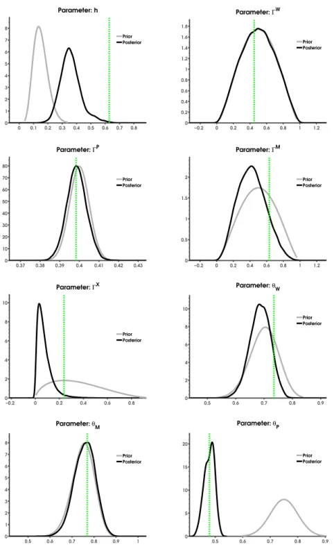
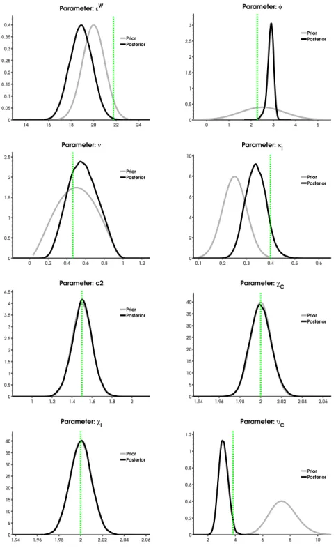
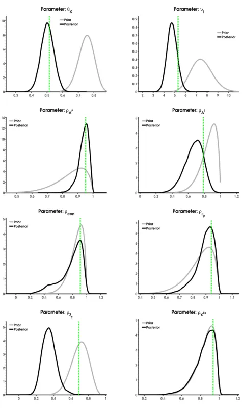
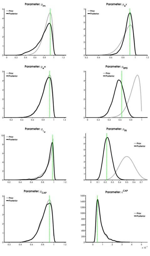
We follow the Bayesian approach for a number of reasons. Firstly, as is well-known the use of priors allows us to introduce presample information and to reduce the dimensionality problem associated with the large parameters to data ratio. Secondly, Bayesian methods have well-known and important com-putational advantages over maximum likelihood in larger DSGE models. That is, the use of simulation provides us with a much easier method to derive the marginal distribution of the parameters in the model than the traditional fre-quentist maximum likelihood approach involving maximisation. The use of pri-ors gives curvature to a highly dimensional likelihood-function, which is likely to be ‡at in many dimensions due to poorly identi…ed parameters. Even the most sophisticated algorithms have a hard time …nding the global maximum of such a function; it is much easier to simulate the posterior distribution of the parameters than to maximize the likelihood function.
Our goal is to report features of the posterior distribution. The Bayesian methodology provides a mapping from the prior distribution to the posterior
through data. Let denote all the parameters in the model we aim to estimate
and let YT denote all the observed data we will use in the estimation. Let
p( )denote the prior distribution over these parameters. The model implies a
likelihoodp YTj and we then have a posterior distribution of given by:
p jYT = p Y
T
j p( )
p(YT) (77)
The posterior distribution equals the prior distribution times the likelihood func-tion divided by a scaling factor. It can perhaps be helpful to think of Bayesian analysis as traditional maximum likelihood with a penalty function in form of
the prior distribution,p( ). That is, the prior distribution assign low values to parameter values which the Bayesian econometrician …nds implausible.
The posterior distribution,p jYT , summarizes the uncertainty regarding
the parameter values. The posterior is di¢ cult to characterize and we con-sequently generate draws from it using a Metropolis-Hastings algorithm. The resulting empirical distribution is used to obtain point estimates, uncertainty bands etc.
4.2
Data and shocks
We estimate the model on data running from 1990 to 2015. We use the …rst 5 years as ’training’ sample for the Bayesian estimation which we afterwards discard in the analysis. This has the advantage that initial conditions in the historical shock decomposition are likely to have vanished in the sample period, see also section (6). We add the most recent forecast produced by National-banken for the 3-year period after the sample to get better estimates of the long term trend in data. The latter must be seen as a consequence of the crisis period which might bias the long-run growth rate downwards leaving a worse …t at the end of our sample. Strictly speaking we should allow for a structural break but we leave that for future work. We use data from 1990 although the european currency union was not in place before 1999. Hence, we weight the costs of having less data less than the costs of using data from a group of coun-tries within a currency union, which was not in place at that point in time. We believe, however, that the initial eurozone countries to some extent shared business cycles already in 1995, as also suggested by Dam [2008].
In estimating the model, we use times series for 23 macroeconomic variables. The following time series for Danish variables are taken from Statistics Denmark
and Nationalbanken:13
Real GDP
Private consumption
Government consumption
in-cluding public production Government investment Exports
Imports
Total investment including in-ventories and construction Labour income tax
Private employment Unemployment (net)
Industry nominal wages de‡ated by CPI
Investment de‡ator PPI index
Import de‡ator Export de‡ator
Danish nominal interest rate
The ’Rest of World’-variables are de…ned as the weighted sum of GDP, in‡a-tion or the policy rate of the Danish trading partners excluding trading partners within the eurozone. The eurozone and the Rest of the World are approximately of equal size. Data is taken from the Ecowin data base and OECD. For the for-eign economies we use the following variables:
In‡ation in the eurozone and in the rest of the world Real GDP in the eurozone and in the rest of the world ECB policy rate
Implied rest of the world policy rate E¤ective exchange rate
Prior to estimation, we transform the time series into quarter-on-quarter growth rates, approximated by the …rst di¤erence of their logarithm. As ex-plained above, in the model, we include a trend in productivity and in the relative price of investments goods. The variables in the model therefore have trends and consequently, we do not demean data. Also, a number of additional transformations are made to ensure that variable measurement is consistent with the properties of the model’s growth path. Firstly, we remove the sample growth rate di¤erentials between the export and import variables and Danish GDP, as these variables in the sample have grown faster than GDP re‡ecting globalisation, see …gure (2) and the discussion in section (2). Secondly, for the e¤ective exchange rate we band-pass …lter and demean the data. Lastly, we HP-…lter data for the foreign economies as we do not model trends in the foreign economies.
Data for Denmark including the e¤ective exchange rate against the rest-of-world is shown in …gures (3), (4) and (5). The time-series used in the estimation for the foreign economies are shown in …gure (6).
4.2.1 Shocks
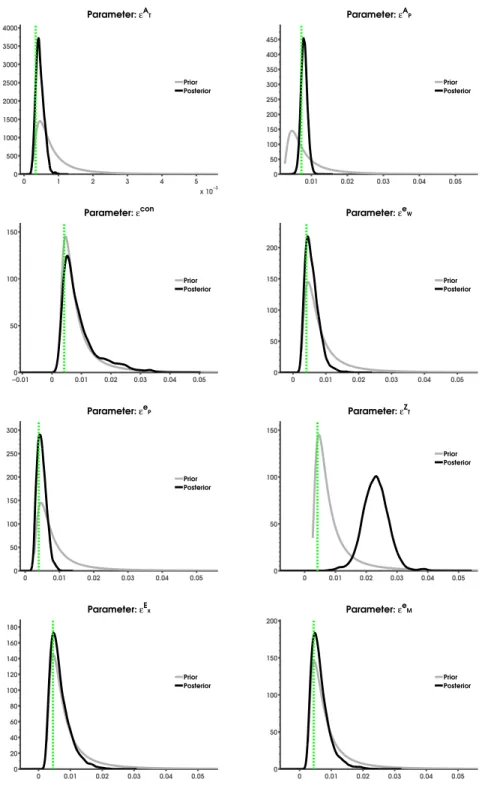
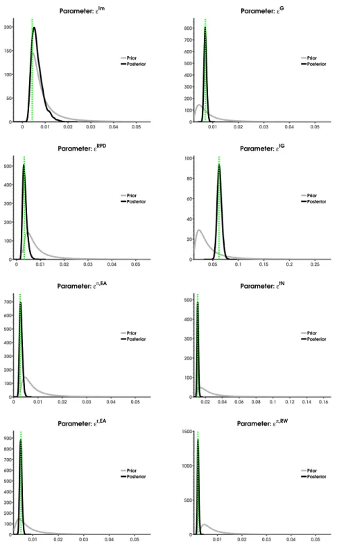
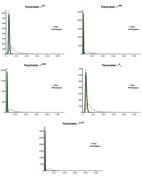
The model includes all in all 27 structural shocks but we only use 22 including the shocks from the exogenous AR-models for public consumption, public in-vestments and labour income tax in the estimation of the model. Finally, we use the 6 shocks from the DSGE-model for the two foreign economies:
Public consumption shock,"G
Perm. tech shock,"AP
Temp. tech shock,"AT
Temp. investment shock,"ZT
Cap. utilization shock,"cap
Consumption shock,"con
Price markup shock,"eP
Export shock,"XEx
Import shock,"Im
Import price markup shock,"eM
Export price markup shock,"eX
Riskpremia shock,"RP D
Public investment shock,"IG
Tax on labour income shock,"tN
EA price shock, "pi;EA
EA output shock,"y;EA
ECB interest rate shock, "r;EA
RoW price shock,"pi;RW
RoW output shock,"y;RW
RoW interest rate shock,"r;RW
UIP shock,"U IP
As already described, all shocks are assumed to feed into …rst-order autore-gressive processes, except for the shock to the ECB policy rate, the shock to the policy rate for the rest of the world, and the UIP shock, which are all white noise, and the shocks to public investment and the labour income tax, which follow higher-order autoregressive processes.
The shocks which are not used in the estimation are shocks to three taxes,
capital income tax,"tK, VAT,"tV AT, and tax on bond income,"tB. These tax
rates have been kept almost …xed throughout the sample but we keep the shocks in the model for policy experiments. We also do not include shocks to the trend
in the relative price of investment goods,"ZP. Lastly, we do not use the labour
supply shock," , as the model is not able to distinguish between this shock and
the wage markup shock in the estimation. In the estimation we assume that all
data are measured with measurement error except for the ECB policy rate.14
4.3
Calibration
It is well known that some parameters in DSGE-models are hard to identify and we do not assume that our model is any di¤er