A Bias-Corrected Fixed Effects Estimator in the
Dynamic Panel Data Model
∗
Chihwa Kao
†Long Liu
‡Rui Sun
§Abstract
In this paper, we proposed a biased-corrected FE estimator for the dynamic panel data model which works for all the autoregressive coefficient values that in (−1,1].We derived the asymptotic distribution of the suggested bias-corrected FE estimator. We showed that it is more efficient than the bias-corrected FD estimator. In addition, when the initial condition is nonstationary, many of the existing dynamic estimators become inconsistent, however, the consistency of the bias-corrected FE estimator we proposed does not depend on the stationary of the initial condition. We also compared the finite sample performances of these estimators using Monte Carlo simulations.
1
Introduction
Many economic issues involve modeling individual behaviors overtime, for example, the dynamic wage equation, employment model, and investment of firms overtime. Panel data offers empirical researchers great opportunities to understand this dynamic behaviors over time. However, using panel data to model this dynamic also creates challenges, one of which is measuring the individual specific effects in conjunction with the dynamic behavioral effects. People tend to consider the fixed effects approach to treat the unobserved effects as parameters to be estimated, therefore allows arbitrary correlation between the unobserved effects and the regressors. However, estimation of the unobserved effects also brings in the incidental parameters problem as first pointed out by Neyman and Scott (1948), where a finite number of observations is used to estimate the incidental parameters. In the case of dynamic panel data model, when the number of observations for the time series is fixed at
T, it is well known that the fixed effects (FE) estimator is inconsistent due to the incidental
∗This paper is dedicated in honour of Badi H. Baltagi’s many contributions to econometrics and in
particular panel data analysis.
†Department of Economics, University of Connecticut, 341 Mansfield Road, Unit 1063, Storrs, CT
06269-1063; [email protected]
‡Department of Economics, University of Texas at San Antonio, 1 UTSA Circle, San Antonio, TX 78249;
email: [email protected]
§Department of Economics, University of Connecticut, 341 Mansfield Road, Unit 1063, Storrs, CT
parameter problem, and so is the first-difference (FD) estimator. A nice review on the dynamic panel data model is available in Baltagi (2013).
The standard solution to this inconsistency problem in dynamic panel model is to imple-ment the instruimple-mental variable (IV) estimation which was first proposed by Anderson and Hsiao (1981, 1982). This strategy is performed based on the first-differenced model, which is free of the individual effects, and estimating the autoregressive coefficient using the lagged dependent variable, either in the form of level or first-differenced, as the instrument. They show that this IV estimator is consistent under n → ∞ or T → ∞ or both. In light of this Anderson-Hsiao estimator, several generalized method of moments (GMM) estimators were proposed, such as Arellano and Bond (1991), Arellano and Bover (1995), Blundell and Bond (1998) where they use all the available lagged dependent variables as instruments, rather than just the first lag. However, these GMM estimators have their drawbacks. First of all, it is well known that these GMM estimators suffer from weak instrument problem when the true value of the autoregressive coefficient is close to one. In the extreme case where the true value equals to one, the instruments become totally irrelevant. Secondly, for these GMM estimators, once we allow the time dimension to grow as the cross-sectional dimension, the number of instruments T(T2−1) → ∞ as T → ∞. Hence the heavy computation burden of these GMM estimators is a drawback for dynamic panel data with large T. Thirdly, when both n and T tend to infinity, Alvarez and Arellano (2003) showed that GMM estimators are consistent but asymptotically biased of order 1/n.
Apart from the GMM estimators, a variety of papers suggest bias-corrected estimators. For example, Han and Phillips (2010) proposed a first differenced least squares (FDLS) estimator. As we showed in Section 2, this FDLS estimator could be viewed as a bias-corrected FD estimator. Later on, Han, Phillips and Sul (2014) further proposed a panel fully aggregated (PFAE) estimator, which is also called X-differencing estimator, to improve efficiency. Both FDLS and PFAE estimators can accommodate the unit root case where
ρ= 1. However, FDLS and PFAE estimator crucially rely on the stationary initial condition assumption. The importance of the initial condition has been studied by previous research such as Kiviet (2005); Chao, Kim and Sul (2014); Hsiao and Zhou (2018). As Chao, Kim and Sul (2014) pointed out when the initial condition is nonstationary, both FDLS and PFAE estimator can be inconsistent.
Besides the bias-corrected FD estimator, existing research also considers to correct the bias of the FE estimator. When T is fixed, the FE estimator is inconsistent due to the incidental parameters problem. As shown in Hahn and Kuersteiner (2002), once we allowT
go to infinity at the same rate as n, we are able to recover the consistency of the dynamic panel FE estimator. The intuition is similar to the explanations provided by Alvarez and Arellano (2003); Baltagi, Kao and Liu (2008, 2012, 2017); Kao (1999) that the bias vanishes completely as T → ∞. However, the asymptotic bias remains and is of order 1/T. Hahn and Kuersteiner (2002) suggested a bias-corrected FE estimator, but for |ρ| <1 only. This bias-corrected FE estimator has been further extended by a series of papers such as Bruno (2005); Bun (2003); Bun and Carree (2005, 2006); Hahn and Moon (2006), to name a few.
In this paper, we extend the bias-corrected FE estimator in Hahn and Kuersteiner (2002) to the case of ρ = 1. In order to bridge the cases for |ρ| < 1 and ρ = 1, following the idea
of Perron and Yabu (2009a,b), we suggest a new bias-corrected FE estimator for all the ρ
values within (−1,1]. This idea of bridge estimator has been applied by Baltagi, Kao and Liu (2014, 2019) in case of panel data with stationary or nonstationary disturbances. We derived the asymptotic distribution of the suggested bias-corrected FE estimator. As an advantage, the consistency of the bias-corrected FE estimator proposed in this paper does not reply on the stationary of the initial condition. We also compared finite sample performance of these estimators using Monte Carlo simulations.
The article is organized as follows. Section 2 introduces the model and reviews the bias-corrected FD estimators in Han and Phillips (2010) and Han, Phillips and Sul (2014). We suggest a bias-corrected FE estimator that is robust to nonstationary initial condition in Section 3. We derive the asymptotic distribution of the proposed estimator, and show that it is more efficient than the bias-corrected FD estimator. Simulation results are presented in Section 4 and Section 5 provides the concluding remarks. Mathematical proofs are contained in the supplemental appendix. A few words on notation. We use (n, T) → ∞ to denote the joint limit. Convergence in probability and distribution are denoted as →p and →d, respectively.
2
The Model and Literature Reviews
We consider the following dynamic panel model as suggested by Han and Phillips (2010) and Han, Phillips and Sul (2014):
yit =αi+uit, (1)
uit =ρui,t−1+it, (2)
for i = 1, ..., , n, t = 1, ..., T, where αi is unobservable individual heterogeneity and it iid
∼
N(0, σ2) with finite fourth moments. The panel autoregressive coefficient ρ∈ (−1,1]. This model could be rewritten into
yit =ρyi,t−1+λi+it (3)
whereλi = (1−ρ)αi. The parameter of interest is the panel autoregressive coefficientρ, and
λi are the nuisance parameters to be estimated. When ρ= 1, this model is free of individual
heterogeneity and when |ρ| < 1 the model we consider here and the usual dynamic panel model are not distinguishable. The stationary initial condition in Han and Phillips (2010) and Han, Phillips and Sul (2014) could be expressed as:
Assumption 1 The autoregressive process uit is initialized at some random quantity ui0 with E(u2
i0)< ∞, allowing for stationary by setting ui0
iid
∼ N(0, σ2
1−ρ2) when |ρ| <1 and for
random recent initialization of the form ui0 = Pkj=1ui,−j for some fixed k when ρ= 1.
It is well known that the FE and FD estimators of ρ are inconsistent when n→ ∞ with fixedT due to the incidental parameters problem. Arellano and Bond (1991), Arellano and Bover (1995) and Blundell and Bond (1998) developed GMM estimators that are popular in
the literature. However, these GMM estimators suffer from the weak IV problem when ρ is close to 1. Therefore, various biased-corrected estimators have been derived as alternative solutions. In particular, Han and Phillips (2010) and Han, Phillips and Sul (2014) suggested estimators that allow |ρ| < 1 or ρ = 1. In the following, we first show that the estimator in Han and Phillips (2010) could be viewed as a bias-corrected FD estimator. We then discussed the drawbacks of these estimators. To see this, note that the first-difference (FD) estimator has the form
ˆ ρF D = Pn i=1 PT t=2∆yi,t−1∆yit Pn i=1 PT t=2(∆yi,t−1) 2 , (4)
where ∆yit =yit−yi,t−1 and ∆yi,t−1 = yi,t−1−yi,t−2. In the following Lemma, we showed
that ˆρF D is inconsistent.
Lemma 1 As (n, T)→ ∞ , under Assumption 1, we have ρˆF D−ρ p
→ −1+2ρ.
Note that Lemma 1 can be rewritten into 2 ˆρF D + 1 p
→ ρ. Therefore, a bias-corrected estimator based on ˆρF D can be suggested as
2 ˆρF D + 1 = 2 Pn i=1 PT t=2∆yi,t−1∆yit Pn i=1 PT t=2(∆yi,t−1) 2 + 1 = Pn i=1 PT t=2∆yi,t−1(2∆yit+ ∆yi,t−1) Pn i=1 PT t=2(∆yi,t−1) 2
which is interestingly the same as the first difference least squares (FDLS) estimator sug-gested in Han and Phillips (2010):
ˆ ρHP = Pn i=1 PT t=2∆yi,t−1(2∆yit+ ∆yi,t−1) Pn i=1 PT t=2(∆yi,t−1) 2 .
In other words, the estimator suggested in Han and Phillips (2010) can be viewed as a bias-corrected FD estimator, which could be easily calculated from ˆρHP = 2 ˆρF D+ 1. As shown
in Theorem 1 of Han and Phillips (2010),
p
n(T −1) ( ˆρHP −ρ) d
→N(0,2 (1 +ρ)) (5)
forρ∈(−1,1] as (n, T)→ ∞. A nice feature of ˆρHP is that its formula is the same for cases
|ρ|<1 and ρ= 1. However, its speed of convergence is still pn(T −1) whenρ= 1, which is slow. To improve the efficiency, Han, Phillips and Sul (2014) extended the estimator in Han and Phillips (2010) and suggested a PFAE estimator, which is also called X-differencing estimator, as ˆ ρHP S = Pn i=1 PT t=4 Pt−3 s=1(yi,t−1−yi,s+1) (yit−yis) Pn i=1 PT t=4 Pt−3 s=1(yi,t−1−yi,s+1) 2 . (6)
Han, Phillips and Sul (2014) showed that if |ρ|<1,
√
nT( ˆρHP S−ρ) d
and if ρ= 1,
√
nT( ˆρHP S−1) d
→N(0,9) (8)
as (n, T)→ ∞. As we can see, when ρ= 1, the speed of convergence of ˆρHP S is
√
nT, which is better than pn(T −1) of ˆρHP.
As Chao, Kim and Sul (2014) pointed out, the stationary initial condition in Assumption 1 is crucial to ˆρHP and ˆρHP S. If the initial condition is nonstationary, both ˆρHP and ˆρHP S
could be inconsistent. For example, if ui0
iid
∼ N(m1, m2) for all i, where m2 > 0, Equation
(17) in Chao, Kim and Sul (2014) showed that
ˆ ρHP S−ρ p → ρ(1−ρ 2) [σ2−m 2(1−ρ2)] m2ρ2(1−ρ2) +σ2(2−ρ2) +O 1 T , (9)
which implies that ˆρHP S is inconsistent unless m2 =σ2/(1−ρ2). Similarly, consistency of
ˆ
ρHP relies on the stationary initial condition, too. As a solution, Chao, Kim and Sul (2014)
suggested a mean average estimator that is a weighted average of the first difference IV estimator and the pooled OLS estimator. However, choosing the weights could be arbitrary, which is an undesirable feature in practice. In the following, we will suggest a bias-corrected Fixed Effects estimator that is robust to the initial condition.
3
The Bias-Corrected Fixed Effects Estimator
In order to eliminate the individual heterogeneity, we normally perform within-transformation by subtracting the time-series mean from the variables. The FE estimator, which is actually the same as the quasi-maximum likelihood estimator (QMLE), has the form
ˆ ρF E = Pn i=1 PT t=1 yi,t−1−yi,−1 (yit−yi) Pn i=1 PT t=1 yi,t−1−yi,−1 2 (10) where yi = 1 T PT t=1yit and yi,−1 = 1 T PT
t=1yi,t−1. However, to eliminate the unobservable
individual heterogeneity by demeaning the variable of interest yi,t−1, we introduce new
en-dogeneity to the transformed regressor, which causes the FE estimator to be inconsistent under small T asymptotics. To see this, let us rewrite Equation (10) into
ˆ ρF E−ρ= 1 n Pn i=1 PT t=1(ui,t−1−ui,−1)it 1 n Pn i=1 PT t=1(ui,t−1−ui,−1) 2 where ui = 1 T PT t=1uit and ui,−1 = 1 T PT
t=1ui,t−1. Following Hahn and Kuersteiner (2002),
we assume the following:
Assumption 2 (i) it ∼iid(0, σ2); (ii)
n T →κ where 0< κ <∞; (iii) 1 n Pn i=1y2i0 =O(1); (iv) n1Pn i=1α 2 i =O(1).
When |ρ|<1, it is easy to show that 1 n n X i=1 T X t=1 (ui,t−1−ui,−1)2 p →T σ 2 1−ρ2 +O(1) and 1 n n X i=1 T X t=1 (ui,t−1−ui,−1)it p → − T X t=1 E(ui,−1it) = − σ2 1−ρ +O 1 T , as n→ ∞. Hence ˆ ρF E−ρ p → − σ2 1−ρ+O 1 T T σu2 1−ρ2 +O(1) =−1 +ρ T +O 1 T2 . (11)
asn→ ∞, which is known as Nickell Bias discussed in Nickell (1981). The bias is nontrivial if the time series dimension T is small, however, the bias decreases in T. Once we move away from fixed T to largeT asymptotics, the FE estimator is consistent even though it is asymptotically biased. To be specific, Hahn and Kuersteiner (2002) showed that if |ρ|<1,
√ nT ˆ ρF E−ρ+ 1 +ρ T d →N 0,1−ρ2, (12)
as (n, T) → ∞, which implies a bias of −(1 +ρ)/T in ˆρF E asymptotically. Hahn and
Kuersteiner (2002) hence suggested a bias-corrected estimator ofρ as
ˆ
ρHK = ˆρF E+
1 + ˆρF E
T (13)
and its asymptotic distribution will be
√
nT ( ˆρHK −ρ) d
→N 0,1−ρ2
as (n, T) → ∞. As we can see, this bias-corrected estimator is asymptotically unbiased, however it is worth pointing out that this estimator only works for the case when|ρ|<1. If
ρ= 1, Theorem 4 in Hahn and Kuersteiner (2002) showed that
√ nT ˆ ρF E−1 + 3 T + 1 d →N 0,51 5 (14)
as (n, T)→ ∞, which implies a bias of −3/(T + 1) in ˆρF E.1 In this case, the bias-corrected
estimator ˆρHK in Equation (13) does not work properly any more. In order to bridge the
cases of |ρ| < 1 and ρ = 1, following the idea of Perron and Yabu (2009a,b); Baltagi, Kao and Liu (2014, 2019), we can suggest a bias-corrected estimator of ρ as follows:
ˆ ρF EBC = ˆ ρF E+ 1+ ˆTρF E if ˆρF E <1− T3+1 1 if ˆρF E ≥1− T+13
1This result for the case ρ= 1 has also been derived in Theorem 2 in Kao (1999), which discusses the
Essentially, we compare two values, i.e., 1−ρˆF E and T+13 , to determine what value to assign
to the bias-corrected estimator. 1−ρˆF E is the difference between one and the estimated value
of FE estimator. T3+1 is the theoretical bias when ρ= 1. The intuition of this bias-corrected is the following: we first assume that the true value of ρ is one, if the estimated bias is less than the theoretical bias, i.e., T3+1, we will set the value of bias-corrected estimator to one. However, if the estimated bias is greater than the theoretical bias ofρ being one, we set the bias-corrected estimator to be ˆρHK in Equation (13), which is the bias-corrected estimator
for the case |ρ| < 1. Consider the case where the time series dimension is relatively large, the term T+13 is going to be a small number. Therefore, if the estimated bias is even smaller than that small theoretical bias of ρ= 1, this is probably a strong evidence supporting that the true value of the parameter is one. In contrast, if the estimated bias is greater than its theoretical bias, this turns out to favor the fact that the true value is not one. The asymptotic results for ˆρF EBC are given in the following theorem:
Theorem 1 As (n, T)→ ∞, under Assumption 2, we have
1. If |ρ|<1, √ nT( ˆρF EBC −ρ) d →N 0,1−ρ2. 2. If ρ= 1, √ nT( ˆρF EBC−1) p →0.
By comparing Theorem 1 to Equations (7) and (8), we can see that when |ρ| < 1, the asymptotic variance of ˆρF EBC is 1−ρ2, which is the same as the asymptotic variance of
ˆ
ρHP S. When ρ = 1, the speed of convergence of ˆρF EBC is
√
nT, which is also the same as the speed of convergence of ˆρHP S. However, the asymptotic distribution of ˆρF EBC is not
available when ρ= 1. From the Monte Carlo simulations in Section 4, we find ˆρF EBC is not
as efficient as ˆρHP S when ρ= 1.
As an important remark, Theorem 1 doesn’t rely on the stationary initial condition in Assumption 1. For example, ifui0
iid
∼ N(m1, m2) for alli, wherem2 >0, Section 3.1 in Chao,
Kim and Sul (2014) showed that Equation (11) still holds. This means, the ˆρF E will have
the same asymptotic bias whether or not the initial observation satisfies m2 =σ2/(1−ρ2).
Therefore, a big advantage of our suggested bias-corrected FE estimator is that it is robust to different initial conditions. We will illustrate it by using Monte Carlo simulations in the next section.
4
Monte Carlo Simulation
In this section, we report the finite sample performance of different dynamic panel data estimators based on the Monte Carlo simulation. Following Han, Phillips and Sul (2014), the data is generated based on the model in Equations (1) and (2), where αi
iid
∼ N(2,1) and
it iid
∼ N(0,1). The true ρwe consider are 0,0.3,0.6,0.9,and 1. Although the time dimension of the panel data is getting larger and larger now in empirical work, but in most of the cases
they are still smaller than the cross-sectional dimension. Therefore, for all the simulations, we consider n ∈ {100,200} and T ∈ {5,10,20,50}.
For a better evaluation of the performance of each estimator, we consider two cases of the initial conditions, i.e., stationary and nonstationary, respectively. For the stationary initial condition, following Han, Phillips and Sul (2014), the data generating processes are initialized at t = −100 such that ui,−100 = 0 for all i and then drop the observations for
t < 0. For the nonstationary initial condition, following Chao, Kim and Sul (2014), the initial values are generated as ui0
iid
∼N(5,1) for alli.
We compare our bias-corrected estimator with several existing dynamic panel estimators. More specifically, we compare the biases and RMSEs among the following estimators:
1. The FE estimator ˆρF E;
2. The FD estimator ˆρF D;
3. The difference GMM estimator in Arellano and Bond (1991) ˆρGM M−DIF;
4. The system GMM estimator in Arellano and Bover (1995) and Blundell and Bond (1998) ˆρGM M−SY S;
5. The estimator in Han and Phillips (2010) ˆρHP, which is also the bias-corrected FD
estimator;
6. The estimator in Han, Phillips and Sul (2014) ˆρHP S, which is the X-differencing
esti-mator;
7. The bias-corrected FE estimator ˆρF EBC.
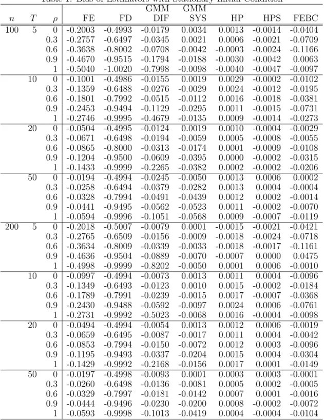
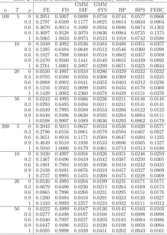
The simulation was performed in Stata. The difference GMM and the system GMM are estimated by the “xtabond” and the “xtdpdsys” commands, respectively, and the X-differencing estimator is obtained by direct calculation using Equation (6). All the results are based on 10,000 replications. Tables 1 and 2 report the bias and RMSE, respectively, for all the estimators with the stationary initial condition. While Tables 3 and 4 report the bias and RMSE, respectively, for all the estimators with the nonstationary initial condition. When the initial condition is stationary, as in Table 1, we can see that FE and FD are largely biased. Both GMM-DIF and GMM-SYS perform well when ρ is small. However, whenρis close to 1, their biases increase sharply due to the weak instrument problem. Both HP and HPS perform well in all situations. When T = 5, their performances are similar. WhenT increases to 10, 20 and 50, HPS outperforms HP. For our proposed FEBC estimator, its bias is larger than HP an HPS when T = 5. When T increases to 10, 20 and 50, its bias reduces very quickly. In Table 2, when n and T are large, we can see that HPS and FEBC have the smallest RMSE for cases of ρ= 0, 0.3 or 0.6. HPS outperforms best when ρ= 0.9 or 1. FEBC is a close second best.
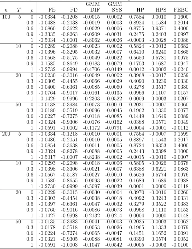
When the initial condition is nonstationary, the same as reported previously for the case of stationary initial condition, largely bias of FE and FD are found in Table 3. GMM-DIF and GMM-SYS still have large bias whenρis close to 1. However, in the case of nonstationary
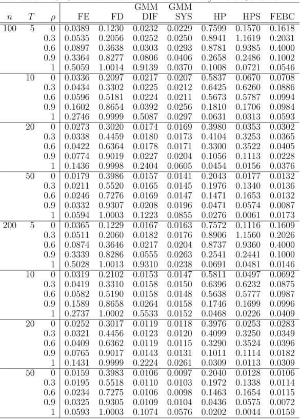
initial condition, the overall performances of HP and HPS in terms of bias drop substantially, which are much larger than FEBC in magnitude. In Table 4, generally speaking, HP and HPS have much larger RMSE than FEBC unless ρ= 1.
Overall, our suggested FEBC estimator performs relatively stable as oppose to other dynamic panel estimators. Especially, when the initial condition is nonstationary and T is large, our estimator outperforms most of the estimators in terms of bias and RMSE. When the initial condition is stationary, FEBC is only slightly worse than HPS. When the initial condition is nonstationary, FEBC dominates other estimators. GMM-DIF and GMM-SYS have large bias whenρ is close to 1. HP and HPS have large bias when the initial condition is nonstationary.
5
Conclusion
In this paper, we propose a bias-corrected FE estimator for dynamic panel model that accommodates the cases when |ρ| < 1 and ρ = 1. We derived its asymptotic distribution and showed that it is more efficient than the bias-corrected FD estimator. More importantly, a nice feature of this bias-correct FE estimator is that its consistency does not depend on the stationary of the initial condition. As we can see from the Monte Carlo simulations, the performance of bias-corrected FE estimator dominates the performances of other existing dynamic panel estimators, especially when the initial condition is nonstationary. While the focus of this paper is to build a bridge for the dynamic panel model to connect cases when
|ρ| < 1 and ρ = 1, it is important to extend this work to dynamic panel data models with other exogenous variables. For this general model, Bun and Carree (2005, 2006) have developed bias-corrected estimators whenρ|<1. The asymptotic bias is a nonlinear function so that Bun and Carree (2005) suggested an iterative procedure as the solution to correct the bias. For this general model with exogenous variables, we can similarly derive the bias for the case when ρ = 1 and therefore suggest a bridge estimator to connect cases when
Table 1: Bias of Estimators with Stationary Initial Condition GMM GMM
n T ρ FE FD DIF SYS HP HPS FEBC
100 5 0 -0.2003 -0.4993 -0.0179 0.0034 0.0013 -0.0014 -0.0404 0.3 -0.2757 -0.6497 -0.0345 0.0021 0.0006 -0.0021 -0.0709 0.6 -0.3638 -0.8002 -0.0708 -0.0042 -0.0003 -0.0024 -0.1166 0.9 -0.4670 -0.9515 -0.1794 -0.0188 -0.0030 -0.0042 0.0063 1 -0.5040 -1.0020 -0.7998 -0.0098 -0.0040 -0.0047 -0.0097 10 0 -0.1001 -0.4986 -0.0155 0.0019 0.0029 -0.0002 -0.0102 0.3 -0.1359 -0.6488 -0.0276 -0.0029 0.0024 -0.0012 -0.0195 0.6 -0.1801 -0.7992 -0.0515 -0.0112 0.0016 -0.0018 -0.0381 0.9 -0.2453 -0.9494 -0.1129 -0.0295 0.0011 -0.0015 -0.0731 1 -0.2746 -0.9995 -0.4679 -0.0135 0.0009 -0.0014 -0.0273 20 0 -0.0504 -0.4995 -0.0124 0.0019 0.0010 -0.0004 -0.0029 0.3 -0.0671 -0.6498 -0.0194 -0.0059 0.0005 -0.0008 -0.0055 0.6 -0.0865 -0.8000 -0.0313 -0.0174 0.0001 -0.0009 -0.0108 0.9 -0.1204 -0.9500 -0.0609 -0.0395 0.0000 -0.0002 -0.0315 1 -0.1433 -0.9999 -0.2265 -0.0382 0.0002 -0.0002 -0.0206 50 0 -0.0194 -0.4994 -0.0245 -0.0050 0.0013 0.0006 0.0002 0.3 -0.0258 -0.6494 -0.0379 -0.0282 0.0013 0.0004 -0.0004 0.6 -0.0328 -0.7994 -0.0491 -0.0439 0.0012 0.0002 -0.0014 0.9 -0.0441 -0.9495 -0.0562 -0.0523 0.0011 -0.0002 -0.0070 1 -0.0594 -0.9996 -0.1051 -0.0568 0.0009 -0.0007 -0.0119 200 5 0 -0.2018 -0.5007 -0.0079 0.0001 -0.0015 -0.0021 -0.0421 0.3 -0.2765 -0.6509 -0.0156 -0.0009 -0.0018 -0.0024 -0.0718 0.6 -0.3634 -0.8009 -0.0339 -0.0033 -0.0018 -0.0017 -0.1161 0.9 -0.4636 -0.9504 -0.0889 -0.0070 -0.0007 0.0000 0.0475 1 -0.4998 -0.9999 -0.8202 -0.0050 0.0001 0.0006 -0.0010 10 0 -0.0997 -0.4994 -0.0073 0.0013 0.0011 0.0004 -0.0096 0.3 -0.1349 -0.6493 -0.0123 0.0010 0.0015 -0.0002 -0.0184 0.6 -0.1789 -0.7991 -0.0239 -0.0015 0.0017 -0.0007 -0.0368 0.9 -0.2430 -0.9488 -0.0592 -0.0097 0.0024 0.0006 -0.0761 1 -0.2731 -0.9992 -0.5023 -0.0068 0.0016 -0.0004 -0.0098 20 0 -0.0494 -0.4994 -0.0054 0.0013 0.0012 0.0006 -0.0019 0.3 -0.0659 -0.6495 -0.0087 -0.0017 0.0011 0.0004 -0.0042 0.6 -0.0853 -0.7994 -0.0150 -0.0072 0.0012 0.0003 -0.0096 0.9 -0.1195 -0.9493 -0.0337 -0.0204 0.0015 0.0004 -0.0304 1 -0.1429 -0.9992 -0.2168 -0.0156 0.0017 0.0001 -0.0149 50 0 -0.0197 -0.4998 -0.0093 0.0001 0.0003 0.0003 -0.0001 0.3 -0.0260 -0.6498 -0.0136 -0.0081 0.0005 0.0002 -0.0005 0.6 -0.0329 -0.7997 -0.0181 -0.0142 0.0007 0.0001 -0.0016 0.9 -0.0444 -0.9496 -0.0230 -0.0200 0.0008 -0.0002 -0.0072 1 -0.0593 -0.9998 -0.1013 -0.0419 0.0004 -0.0004 -0.0104
Table 2: RMSE of Estimators with Stationary Initial Condition GMM GMM
n T ρ FE FD DIF SYS HP HPS FEBC
100 5 0 0.2051 0.5007 0.0899 0.0758 0.0744 0.0577 0.0666 0.3 0.2797 0.6509 0.1177 0.0825 0.0814 0.0634 0.0904 0.6 0.3670 0.8014 0.1680 0.0834 0.0886 0.0674 0.1302 0.9 0.4697 0.9528 0.3070 0.0836 0.0984 0.0725 0.1575 1 0.5065 1.0033 0.8973 0.0524 0.1018 0.0742 0.0580 10 0 0.1049 0.4992 0.0536 0.0484 0.0486 0.0351 0.0357 0.3 0.1395 0.6494 0.0648 0.0512 0.0546 0.0360 0.0398 0.6 0.1827 0.7998 0.0848 0.0518 0.0602 0.0357 0.0509 0.9 0.2470 0.9500 0.1441 0.0549 0.0655 0.0339 0.0892 1 0.2761 1.0001 0.5087 0.0299 0.0671 0.0325 0.0634 20 0 0.0550 0.4997 0.0310 0.0286 0.0329 0.0232 0.0232 0.3 0.0705 0.6500 0.0356 0.0306 0.0369 0.0231 0.0235 0.6 0.0888 0.8002 0.0441 0.0352 0.0403 0.0212 0.0236 0.9 0.1216 0.9502 0.0699 0.0491 0.0434 0.0170 0.0360 1 0.1439 1.0002 0.2360 0.0478 0.0439 0.0151 0.0376 50 0 0.0242 0.4995 0.0366 0.0236 0.0211 0.0148 0.0148 0.3 0.0293 0.6495 0.0494 0.0411 0.0241 0.0141 0.0141 0.6 0.0349 0.7995 0.0589 0.0553 0.0266 0.0122 0.0123 0.9 0.0449 0.9496 0.0630 0.0595 0.0284 0.0084 0.0111 1 0.0598 0.9997 0.1089 0.0636 0.0293 0.0062 0.0179 200 5 0 0.2043 0.5015 0.0657 0.0534 0.0538 0.0420 0.0571 0.3 0.2786 0.6516 0.0861 0.0579 0.0594 0.0467 0.0827 0.6 0.3651 0.8016 0.1171 0.0568 0.0647 0.0494 0.1235 0.9 0.4649 0.9510 0.1838 0.0533 0.0696 0.0505 0.1327 1 0.5010 1.0006 0.9179 0.0361 0.0713 0.0513 0.0180 10 0 0.1020 0.4997 0.0358 0.0326 0.0351 0.0246 0.0259 0.3 0.1367 0.6496 0.0419 0.0342 0.0387 0.0250 0.0305 0.6 0.1801 0.7994 0.0530 0.0336 0.0418 0.0242 0.0435 0.9 0.2438 0.9491 0.0876 0.0319 0.0457 0.0227 0.0809 1 0.2737 0.9995 0.5455 0.0200 0.0475 0.0228 0.0369 20 0 0.0520 0.4995 0.0204 0.0199 0.0231 0.0171 0.0171 0.3 0.0679 0.6496 0.0230 0.0215 0.0264 0.0169 0.0173 0.6 0.0865 0.7996 0.0268 0.0231 0.0295 0.0151 0.0178 0.9 0.1200 0.9494 0.0416 0.0291 0.0323 0.0120 0.0327 1 0.1433 0.9993 0.2257 0.0210 0.0332 0.0111 0.0312 50 0 0.0222 0.4999 0.0167 0.0130 0.0145 0.0103 0.0103 0.3 0.0277 0.6498 0.0197 0.0168 0.0167 0.0098 0.0098 0.6 0.0340 0.7997 0.0227 0.0203 0.0185 0.0084 0.0086 0.9 0.0447 0.9496 0.0255 0.0230 0.0198 0.0058 0.0094 1 0.0595 0.9998 0.1039 0.0451 0.0202 0.0043 0.0161
Table 3: Bias of Estimators with Nonstationary Initial Condition GMM GMM
n T ρ FE FD DIF SYS HP HPS FEBC
100 5 0 -0.0334 -0.1208 -0.0015 0.0002 0.7584 0.0010 0.1600 0.3 -0.0488 -0.2038 -0.0019 0.0003 0.8924 1.1584 0.2014 0.6 -0.0860 -0.3622 -0.0029 -0.0006 0.8755 0.9371 0.4000 0.9 -0.3335 -0.8263 -0.0209 -0.0031 0.2475 0.2403 0.0997 1 -0.5034 -1.0001 -0.8062 -0.0026 -0.0003 -0.0028 -0.0086 10 0 -0.0289 -0.2088 -0.0023 0.0002 0.5824 -0.0012 0.0682 0.3 -0.0396 -0.3295 -0.0032 -0.0007 0.6410 0.6240 0.0865 0.6 -0.0568 -0.5175 -0.0049 -0.0022 0.5650 0.5781 0.0975 0.9 -0.1585 -0.8649 -0.0183 -0.0079 0.1703 0.1687 0.0947 1 -0.2732 -0.9994 -0.4706 -0.0149 0.0012 -0.0002 -0.0240 20 0 -0.0230 -0.3016 -0.0049 0.0002 0.3968 -0.0017 0.0259 0.3 -0.0305 -0.4455 -0.0066 -0.0029 0.4090 0.3239 0.0330 0.6 -0.0400 -0.6361 -0.0085 -0.0060 0.3278 0.3517 0.0380 0.9 -0.0764 -0.9017 -0.0161 -0.0135 0.0966 0.1107 0.0157 1 -0.1429 -0.9996 -0.2303 -0.0522 0.0009 0.0003 -0.0207 50 0 -0.0138 -0.3984 -0.0073 -0.0010 0.2031 -0.0007 0.0060 0.3 -0.0180 -0.5519 -0.0096 -0.0045 0.1962 0.1330 0.0077 0.6 -0.0227 -0.7275 -0.0118 -0.0085 0.1449 0.1649 0.0089 0.9 -0.0324 -0.9306 -0.0176 -0.0162 0.0388 0.0571 0.0049 1 -0.0591 -1.0002 -0.1172 -0.0791 -0.0004 -0.0001 -0.0112 200 5 0 -0.0334 -0.1218 -0.0010 0.0001 0.7564 -0.0007 0.1599 0.3 -0.0486 -0.2051 -0.0010 0.0005 0.8897 1.1543 0.2017 0.6 -0.0854 -0.3638 -0.0011 0.0005 0.8724 0.9353 0.4000 0.9 -0.3324 -0.8278 -0.0088 -0.0005 0.2443 0.2398 0.1000 1 -0.5017 -1.0007 -0.8238 -0.0002 -0.0015 -0.0019 -0.0007 10 0 -0.0293 -0.2098 -0.0018 -0.0006 0.5805 -0.0026 0.0678 0.3 -0.0398 -0.3306 -0.0021 -0.0007 0.6388 0.6221 0.0863 0.6 -0.0567 -0.5187 -0.0027 -0.0010 0.5626 0.5774 0.0976 0.9 -0.1580 -0.8655 -0.0093 -0.0022 0.1689 0.1689 0.0988 1 -0.2730 -0.9999 -0.5097 -0.0039 0.0001 0.0000 -0.0118 20 0 -0.0229 -0.3015 -0.0030 -0.0004 0.3970 -0.0016 0.0260 0.3 -0.0303 -0.4454 -0.0038 -0.0018 0.4092 0.3243 0.0331 0.6 -0.0397 -0.6361 -0.0047 -0.0032 0.3279 0.3522 0.0383 0.9 -0.0760 -0.9016 -0.0086 -0.0073 0.0968 0.1110 0.0153 1 -0.1427 -0.9998 -0.2132 -0.0214 0.0004 0.0000 -0.0148 50 0 -0.0135 -0.3983 -0.0041 -0.0003 0.2035 -0.0003 0.0062 0.3 -0.0178 -0.5518 -0.0053 -0.0026 0.1965 0.1333 0.0079 0.6 -0.0224 -0.7274 -0.0065 -0.0047 0.1451 0.1652 0.0091 0.9 -0.0321 -0.9305 -0.0088 -0.0081 0.0390 0.0574 0.0052 1 -0.0591 -1.0003 -0.1047 -0.0542 -0.0005 -0.0003 -0.0100
Table 4: RMSE of Estimators with Nonstationary Initial Condition GMM GMM
n T ρ FE FD DIF SYS HP HPS FEBC
100 5 0 0.0389 0.1230 0.0232 0.0229 0.7599 0.1570 0.1618 0.3 0.0535 0.2056 0.0252 0.0250 0.8941 1.1619 0.2031 0.6 0.0897 0.3638 0.0303 0.0293 0.8781 0.9385 0.4000 0.9 0.3364 0.8277 0.0806 0.0406 0.2658 0.2486 0.1002 1 0.5059 1.0014 0.9139 0.0370 0.1008 0.0721 0.0546 10 0 0.0336 0.2097 0.0217 0.0207 0.5837 0.0670 0.0708 0.3 0.0434 0.3302 0.0225 0.0212 0.6425 0.6260 0.0886 0.6 0.0596 0.5181 0.0224 0.0211 0.5673 0.5787 0.0994 0.9 0.1602 0.8654 0.0392 0.0256 0.1810 0.1706 0.0984 1 0.2746 0.9999 0.5087 0.0297 0.0631 0.0313 0.0593 20 0 0.0273 0.3020 0.0174 0.0169 0.3980 0.0353 0.0302 0.3 0.0338 0.4459 0.0180 0.0173 0.4104 0.3253 0.0365 0.6 0.0422 0.6364 0.0178 0.0171 0.3300 0.3522 0.0405 0.9 0.0774 0.9019 0.0227 0.0204 0.1056 0.1113 0.0228 1 0.1436 0.9998 0.2404 0.0605 0.0454 0.0156 0.0376 50 0 0.0179 0.3986 0.0157 0.0141 0.2043 0.0177 0.0132 0.3 0.0211 0.5520 0.0165 0.0145 0.1976 0.1340 0.0136 0.6 0.0246 0.7276 0.0169 0.0147 0.1471 0.1653 0.0132 0.9 0.0332 0.9307 0.0208 0.0196 0.0471 0.0574 0.0087 1 0.0594 1.0003 0.1223 0.0855 0.0276 0.0061 0.0173 200 5 0 0.0365 0.1229 0.0167 0.0163 0.7572 0.1116 0.1609 0.3 0.0511 0.2060 0.0182 0.0176 0.8906 1.1560 0.2026 0.6 0.0874 0.3646 0.0217 0.0204 0.8737 0.9360 0.4000 0.9 0.3339 0.8286 0.0555 0.0263 0.2541 0.2441 0.1000 1 0.5028 1.0013 0.9310 0.0238 0.0691 0.0481 0.0146 10 0 0.0319 0.2102 0.0153 0.0147 0.5811 0.0497 0.0692 0.3 0.0419 0.3310 0.0158 0.0150 0.6396 0.6232 0.0875 0.6 0.0582 0.5190 0.0158 0.0148 0.5638 0.5777 0.0987 0.9 0.1589 0.8658 0.0264 0.0158 0.1746 0.1699 0.0996 1 0.2737 1.0002 0.5533 0.0152 0.0468 0.0226 0.0409 20 0 0.0252 0.3017 0.0119 0.0118 0.3976 0.0253 0.0283 0.3 0.0321 0.4456 0.0123 0.0120 0.4099 0.3250 0.0349 0.6 0.0409 0.6362 0.0119 0.0115 0.3290 0.3524 0.0396 0.9 0.0765 0.9017 0.0143 0.0131 0.1011 0.1114 0.0182 1 0.1431 0.9999 0.2224 0.0261 0.0309 0.0113 0.0309 50 0 0.0159 0.3983 0.0106 0.0097 0.2040 0.0128 0.0106 0.3 0.0195 0.5518 0.0110 0.0103 0.1972 0.1338 0.0114 0.6 0.0234 0.7275 0.0106 0.0098 0.1463 0.1654 0.0115 0.9 0.0325 0.9305 0.0109 0.0104 0.0436 0.0575 0.0072 1 0.0593 1.0003 0.1074 0.0576 0.0202 0.0044 0.0159
References
Alvarez, Javier, and Manuel Arellano. 2003. “The Time Series and Cross-Section
Asymptotics of Dynamic Panel Data Estimators.” Econometrica, 71(4): 1121–1159.
Anderson, Theodore Wilbur, and Cheng Hsiao.1981. “Estimation of Dynamic Models
with Error Components.” Journal of the American Statistical Association, 76(375): 598– 606.
Anderson, Theodore Wilbur, and Cheng Hsiao. 1982. “Formulation and estimation
of dynamic models using panel data.” Journal of Econometrics, 18(1): 47–82.
Arellano, Manuel, and Olympia Bover. 1995. “Another look at the instrumental
vari-able estimation of error-components models.”Journal of Econometrics, 68(1): 29–51.
Arellano, Manuel, and Stephen Bond. 1991. “Some Tests of Specification for Panel
Data: Monte Carlo Evidence and an Application to Employment Equations.”The Review of Economic Studies, 58(2): 277–297.
Baltagi, Badi H. 2013. Econometric analysis of panel data. John Wiley & Sons.
Baltagi, Badi H., Chihwa Kao, and Long Liu. 2008. “Asymptotic properties of
esti-mators for the linear panel regression model with random individual effects and serially correlated errors: the case of stationary and non-stationary regressors and residuals.”The
Econometrics Journal, 11(3): 554–572.
Baltagi, Badi H., Chihwa Kao, and Long Liu. 2012. “On the estimation and testing
of fixed effects panel data models with weak instruments.” In 30th Anniversary Edition. 199–235. Emerald Group Publishing Limited.
Baltagi, Badi H., Chihwa Kao, and Long Liu. 2014. “Test of Hypotheses in a Time
Trend Panel Data Model with Serially Correlated Error Component Disturbances.” In
Essays in Honor of Peter C. B. Phillips. Vol. 33 of Advances in Econometrics, 347–394.
Emerald Publishing Ltd.
Baltagi, Badi H., Chihwa Kao, and Long Liu. 2017. “Estimation and identification
of change points in panel models with nonstationary or stationary regressors and error term.”Econometric Reviews, 36(1-3): 85–102.
Baltagi, Badi H., Chihwa Kao, and Long Liu.2019. “Testing for Shifts in a Time Trend
Panel Data Model with Serially Correlated Error Component Disturbance.”Econometric Reviews. forthcoming.
Blundell, Richard, and Stephen Bond.1998. “Initial conditions and moment restrictions
in dynamic panel data models.”Journal of Econometrics, 87(1): 115–143.
Bruno, Giovanni SF. 2005. “Approximating the bias of the LSDV estimator for dynamic
Bun, Maurice JG.2003. “Bias correction in the dynamic panel data model with a nonscalar disturbance covariance matrix.” Econometric Reviews, 22(1): 29–58.
Bun, Maurice JG, and Martin A Carree.2005. “Bias-corrected estimation in dynamic
panel data models.”Journal of Business & Economic Statistics, 23(2): 200–210.
Bun, Maurice JG, and Martin A Carree.2006. “Bias-corrected estimation in dynamic
panel data models with heteroscedasticity.”Economics Letters, 92(2): 220–227.
Chao, John, Myungsup Kim, and Donggyu Sul. 2014. “Mean Average Estimation of
Dynamic Panel Models with Nonstationary Initial Condition.” Essays in Honor of Peter C. B. Phillips, Chapter 8, 241–279.
Hahn, Jinyong, and Guido Kuersteiner. 2002. “Asymptotically Unbiased Inference for
a Dynamic Panel Model with Fixed Effects when BothnandT Are Large.”Econometrica, 70(4): 1639–1657.
Hahn, Jinyong, and Hyungsik Roger Moon.2006. “Reducing bias of MLE in a dynamic
panel model.”Econometric Theory, 22(3): 499–512.
Han, Chirok, and Peter C. B. Phillips. 2010. “GMM Estimation for Dynamic Panels
with Fixed Effects and Strong Instruments at Unity.”Econometric Theory, 26(1): 119–151.
Han, Chirok, Peter C. B. Phillips, and Donggyu Sul. 2014. “X-Differencing and
Dynamic Panel Model Estimation.” Econometric Theory, 30(1): 201–251.
Hsiao, Cheng, and Qiankun Zhou. 2018. “Incidental parameters, initial conditions and
sample size in statistical inference for dynamic panel data models.”Journal of Economet-rics, 207(1): 114–128.
Kao, Chihwa.1999. “Spurious regression and residual-based tests for cointegration in panel data.”Journal of Econometrics, 90(1): 1–44.
Kiviet, Jan F. 2005. “Judging contending estimators by simulation: tournaments in
dy-namic panel data models.” In The refinement of econometric estimation and test
proce-dures. 282–318. Cambridge: Cambridge University Press.
Neyman, J., and Elizabeth L. Scott. 1948. “Consistent Estimates Based on Partially
Consistent Observations.” Econometrica, 16(1): 1–32.
Nickell, Stephen. 1981. “Biases in Dynamic Models with Fixed Effects.” Econometrica,
49(6): 1417–1426.
Perron, Pierre, and Tomoyoshi Yabu.2009a. “Estimating deterministic trends with an
integrated or stationary noise component.”Journal of Econometrics, 151(1): 56–69.
Perron, Pierre, and Tomoyoshi Yabu. 2009b. “Testing for shifts in trend with an
integrated or stationary noise component.” Journal of Business & Economic Statistics, 27(3): 369–396.
A
Proof of Lemma 1
Proof. From Equation (4), we have
ˆ ρF D−ρ= Pn i=1 PT t=2∆yi,t−1∆it Pn i=1 PT t=2(∆yi,t−1) 2 = 1 n(T−1) Pn i=1 PT t=2∆ui,t−1∆it 1 n(T−1) Pn i=1 PT t=2(∆ui,t−1) 2 (15)
where ∆yit=yit−yi,t−1, ∆yi,t−1 =yi,t−1−yi,t−2, ∆uit=uit−ui,t−1, ∆ui,t−1 =ui,t−1−ui,t−2
and ∆it =it−i,t−1. Since
∆uit=it−(1−ρ) ∞ X
j=1
ρj−1i,t−j
for all ρ∈(−1,1], we have
1 n(T −1) n X i=1 T X t=2 (∆ui,t−1)2 = 1 nT n X i=1 T X t=2 " 2i,t−1+ (1−ρ)2 ∞ X j=1 ρ2(j−1)2i,t−1−j−2 (1−ρ) ∞ X j=1 ρj−1i,t−1i,t−1−j # p →σ2+ (1−ρ) 2 1−ρ2 σ 2 = 2 1 +ρσ 2 and 1 n(T −1) n X i=1 T X t=2 ∆ui,t−1∆it = 1 n(T −1) n X i=1 T X t=2 i,t−1−(1−ρ) ∞ X j=1 ρj−1i,t−1−j ! (it−i,t−1) p → −σ2. as (n, T)→ ∞. It follows that ˆ ρF D−ρ= 1 n(T−1) Pn i=1 PT t=2∆ui,t−1∆it 1 n(T−1) Pn i=1 PT t=2(∆ui,t−1) 2 p → −σ 2 2 1+ρσ2 =−1 +ρ 2 (16)
B
Proof of Theorem 1
Proof. Let S = {(T + 1) (1−ρˆF E)>3} and ¯S = {(T + 1) (1−ρˆF E)≤3}. Consider (1).
When |ρ|<1, it suffices to show that
√ nT ( ˆρF EBC−ρ)− √ nT ˆ ρF E −ρ+ 1 + ˆρF E T =√nT ˆ ρF EBC−ρˆF E − 1 + ˆρF E T p →0. We have lim (n,T)→∞Pr √ nT ˆ ρF EBC −ρˆF E − 1 + ˆρF E T > = lim (n,T)→∞Pr √ nT ˆ ρF EBC −ρˆF E− 1 + ˆρF E T > |S Pr (S) + lim (n,T)→∞Pr √ nT ˆ ρF EBC −ρˆF E− 1 + ˆρF E T > |S¯ Pr ¯S.
The first term is zero given that, if S is true, we have ˆρF EBC = ˆρF E + 1+ ˆTρF E so that
Pr √ nT ρˆF EBC−ρˆF E − 1+ ˆTρF E > |S
= 0. The second term is zero since√nT ρˆF E−ρ+ 1+Tρ = Op(1) implies (T + 1) (1−ρˆF E)−3 = (T + 1) (1−ρ)− r T n T + 1 T √ nT ˆ ρF E−ρ+ 1 +ρ T −3 + T + 1 T (1 +ρ) = (T + 1) (1−ρ) +Op r T n ! +Op T + 1 T → ∞
and hence Pr ¯S→0 as T → ∞. Therefore, Pr √ nT ρˆF EBC−ρˆF E −1+ ˆTρF E > →0 as (n, T)→ ∞.
Consider (2). When ρ= 1, we have
lim (n,T)→∞Pr √ nT( ˆρF EBC−1) > = lim (n,T)→∞Pr √ nT( ˆρF EBC −1) > |S Pr (S) + lim (n,T)→∞Pr √ nT( ˆρF EBC −1) > |S¯ Pr ¯S.
Now the fact that √nT ρˆF E −1 + T3+1
= Op(1) implies Pr (S) → 0 as (n, T) → ∞,
so that the first term is zero. For the second term, if ¯S is true, ˆρF EBC = 1 so that
Pr √ nT ( ˆρF EBC −1) > | ¯ S= 0. Thus, Pr (|√nT( ˆρF EBC −1)|> )→0 as (n, T)→ ∞.