A Performance Model For Gpu Architectures: Analysis And Design Of Fundamental Algorithms

(1)

A PERFORMANCE MODEL FOR GPU ARCHITECTURES: ANALYSIS AND DESIGN OF FUNDAMENTAL ALGORITHMS

A THESIS SUBMITTED TO THE GRADUATE DIVISION OF THE UNIVERSITY OF HAWAI‘I AT M ¯ANOA IN PARTIAL FULFILLMENT

OF THE REQUIREMENTS FOR THE DEGREE OF DOCTOR OF PHILOSOPHY IN COMPUTER SCIENCE MAY 2018 By Ben Karsin Thesis Committee: Nodari Sitchinava, Chairperson

Henri Casanova Lipyeow Lim

Jason Leigh Philip von Doetinchem

(2)

Copyright c2018 by Ben Karsin

(3)

ACKNOWLEDGMENTS

First, I would like to thank my wife, Kelsey, for being patient and supportive during my long journey into Academia. I would also like to thank my advisor, Nodari Sitchinava, for guiding me in this work and encouraging me to dedicate myself to the field. I would like to thank Henri Casanova for starting me down this path and for constantly lending his vast knowledge. I would also like to thank my dissertation committee members, Lipyeow Lim, Jason Leigh, and Philip von Doetinchem. Finally, I would like to thank Kyle Berney for the helpful discussions related to this work.

(4)

ABSTRACT

Over the past decade, “many-core” architectures have become a crucial resources for solving com-putationally challenging problems. These systems rely on hundreds or thousands of simple compute cores to achieve high computational throughput. However, their divergence from traditional CPUs makes existing algorithms and models inapplicable. Thus, developers rely on a set of heuristics and hardware-dependent rules of thumb to develop algorithms for many-core systems, such as GPUs.

This dissertation attempts to remedy this by presenting the Synchronous Parallel Throughput (SPT) model, a general performance model that aims to capture the factors that most impact algorithm performance on many-core architectures. The model focuses on two factors that often create performance bottlenecks: memory latency and synchronization overhead. We instantiate the SPT model on three separate modern GPU platforms using a series of microbenchmarks that measure hardware parameters such as memory access latency and peak bandwidth. We further show how multiplicity affects performance by hiding latencies and increasing overall throughput. We consider three fundamental problems as case studies in this dissertation: general matrix-matrix multiplication, searching, and sorting. Using our SPT model, we analyze a state-of-the-art library implementation of a matrix multiplication algorithm and show that our model can generate run-time estimates with an average error of 5% across our GPU platforms. We then consider the problem of batched predecessor search in the context of two levels of the GPU memory hierarchy. In slow, global memory, we demonstrate the accuracy of the SPT model, while in fast, shared memory, we determine that the memory access patterns create a performance bottleneck that de-grades performance. We develop a new searching algorithm that improves the access pattern and increases performance by up to 293% on our GPUs. Finally, we look at comparison-based sort-ing on GPUs by analyzsort-ing two state-of-the-art algorithms and, ussort-ing our SPT model, determine that they each suffer from bottlenecks that stifle performance. With these bottlenecks in mind, we develop GPU-MMS, our GPU-efficient multiway mergesort algorithm, and demonstrate that it outperforms highly optimized library implementations of existing algorithms by an average of 21% when sorting random inputs and up to 67% on worst-case input permutations. These case studies demonstrate both the accuracy and applicability of the SPT model for analyzing and developing GPU-efficient algorithms.

(5)

LIST OF TABLES

3.1 Parameters defined by the hardware system. . . 26

3.2 Parameters defined by the algorithm. . . 26

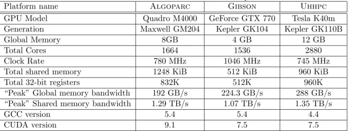
4.1 Details of our three GPU hardware platforms. . . 28

4.2 Hardware details and measured parameters for our three GPU platforms. Parameters marked with * are empirically measured. . . 37

(11)

LIST OF FIGURES

1.1 High-level view of the Intel Xeon Phi processor architecture. Each core has a vector processor that can operate on many elements per cycle. . . 2

1.2 High-level view of the architecture of NVIDIA GPUs. GPUs have a series of stream-ing multiprocessors (SMs), each of which has many cores. . . 2

1.3 Illustration of shared memory access patterns that result in no bank conflicts. . . 5

1.4 When multiple threads access the same shared memory bank, a conflict occurs and accesses are serialized. . . 5

2.1 Illustration of the Parallel External Memory (PEM) model [9]. . . 10

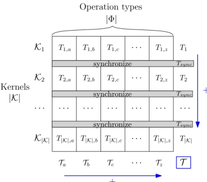
3.1 Illustration of how we model the runtime, T, of an algorithm with|K| kernels, on an architecture with a the set of Φ operation types. . . 18

3.2 Illustration of the BSP model [78] and how our SPT model differs. In the SPT model, we estimate the runtime of each kernel by the time needed to access each type of memory (memories a,b,c, and din this example). . . 22

3.3 Illustration of the DMM and UMM models developed by Nakano [61]. The inter-connection of the address line between the memory management unit (MMU) and memory banks (MBs) results in different optimal memory access patterns. . . 23

3.4 Illustration of the HMM model that combines several DMMs (shared memory) with a UMM (global memory) into a hierarchy. . . 24

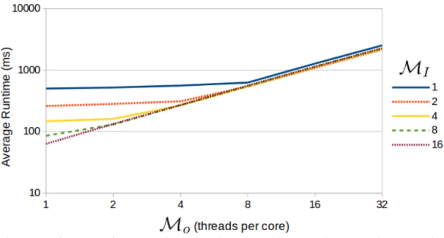
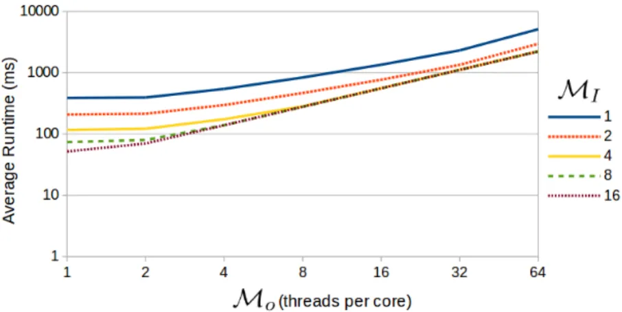
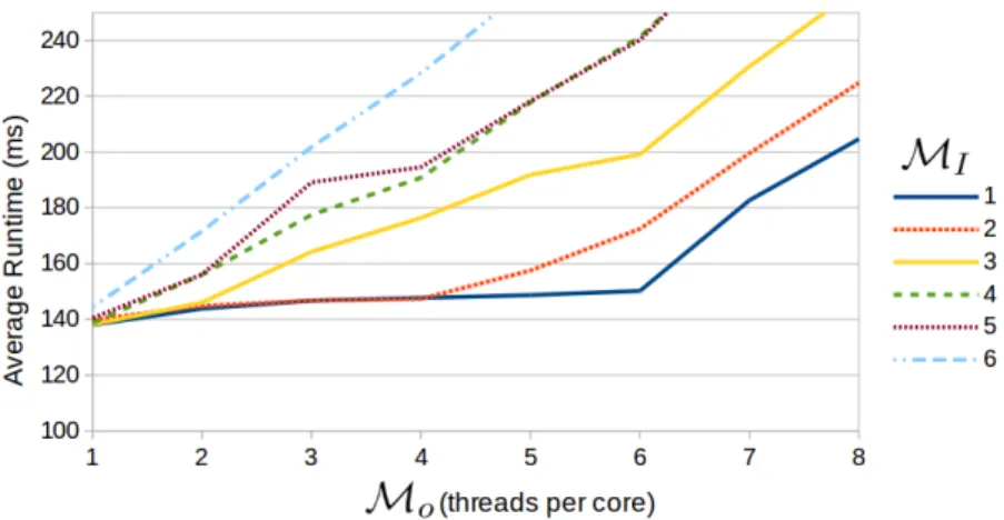
4.1 Impact of oversubscription (Mo) and ILP (MI) on global memory access time. Results on AlgoparcwithN = 216 integers per thread. Once M= 8, peak global memory bandwidth is reached. . . 29

4.2 Impact of oversubscription (Mo) and ILP (MI) on shared memory access time on Algoparcwith N = 215 elements per thread andX= 100. . . 31 4.3 Impact of oversubscription (Mo) and ILP (MI) on time to perform register

oper-ations on Algoparc with N = 215· MI elements per thread and X = 500. Since memory accesses increase withM, multiplicity continues to hide latency as long as runtime remains flat. . . 32

(12)

4.4 Average time persyncthreadsoperation, when performing a fixedN = 105register additions per block, for different values of M_o, on Algoparc. . . 33 4.5 Average runtime to perform N additions and a varying number of deviceSync

operations, for different values of M_o and M_I, on Algoparc. Each deviceSync has a fixed cost, regardless of other parameters. . . 34

4.6 Average time spent per deviceSync, for varying total number of deviceSync operations, and for different values ofMo, onAlgoparc. As we increase the number of deviceSync operations, the time per sync converges to a constant, which we estimate to be Lsync. . . 35

5.1 Illustration of the work done by a single TB in themagma-gemm algorithm. . . 39

5.2 Measured runtime, compared with our model estimate, forn=m= 104 and varying k onAlgoparc. . . 44

5.3 Measured runtime and our model estimate, for n=m=k= 104 and varying NT B on Algoparc. The dotted line shows our model if take into account the impact of using local memory when each thread requires too many registers. . . 45

5.4 Measured runtime and our model estimate, for n=m=k= 104 and varying NT B on Algoparc. The dotted line shows our model if take into account the impact of using local memory when each thread requires too many registers. . . 45

6.1 Measured and estimated runtime when querying different search tree layouts on Gibson withN = 228 and varying number of queries (Q). . . 52 6.2 Measured and estimated runtime when querying different search tree layouts on

Uhhpc withN = 228 and varying number of queries (Q). . . 52 6.3 Measured and estimated runtime when querying different search tree layouts on

Algoparcwith N = 228 and varying number of queries (Q). . . 53 6.4 Worst-case example for the first logN−logwiterations of the PBS algorithm, when

N is a multiple ofw2 (Corollary 6.2.1). . . 56 6.5 Illustration of the shared memory access pattern for stage 1 of the PBS-CF algorithm

(δ≥w). . . 57

6.6 Illustration of the shared memory access pattern for stage 2 of the PBS-CL algorithm (δ < w), for a worst-case example. . . 58

(13)

6.7 Execution time results of our three batched predecessor search implementations for varying numbers of search keys and Q= 500M on Gibson. . . 60

7.1 Estimated and measured MGPU mergesort throughput when varying E (elements per thread) on Algoparc, forN = 100M. . . 66

7.2 Estimated percentage of MGPU mergesort runtime due to each type of operation on Algoparc, for varyingN and E= 31. . . 66

7.3 Estimated and measured MGPU mergesort throughput when varying N on Algo-parc, for both E = 15 and E= 31. . . 67

7.4 High-level illustration of the multiway mergesort algorithm used by Koike and Sadakane [47]. Example depicts multiway mergesort process ifK = 3. . . 68

7.5 Estimated percentage of Koike and Sadakane’s multiway mergesort is due to global memory and shared memory accesses, on Algoparc with N = 229 for varying K values. . . 70

7.6 Example a minBlockHeap structure with w = 4. We perform a fillEmptyNode operation on node v by merging its children, leavingx empty. . . 73

7.7 Estimated throughput of GPU-MMS, compared with the measured performance on AlgoparcwithN = 228 for a range ofK values. Estimated throughput also shown for Koike and Sadakane’ multiway mergesort [47]. . . 77

7.8 Estimated percentage of GPU-MMS execution time that is due each aspect of the algorithm, on Algoparcwith K= 16, for varying input sizesN. . . 77

7.9 Comparison of average throughput for each sorting algorithm on inputs of random integers on Algoparc(middle), Gibson(left), and Uhhpc (right). . . 78

(14)

CHAPTER 1

INTRODUCTION

In recent years, massively parallel, “many-core” architectures have become increasingly popular for solving computationally challenging problems [76, 65, 44, 64]. These architectures, which include modern Graphics Processing Units (GPUs) [44] and Intel Xeon Phi processors [38], are composed of thousands of simple compute cores and are designed to deliver high computational throughput, enabling them to outperform traditional CPUs for many applications [11, 58, 68]. For some applica-tions, these architectures can achieve an order-of-magnitude performance speedup over comparable CPU systems. However, no general model is available to accurately analyze the performance of algorithms on these types of systems. In fact, many details, such as the memory hierarchy and execution pipeline, are not well understood, forcing algorithm designers to rely on heuristics and trial-and-error methods.

This dissertation aims to remedy these shortcomings by proposing a general model that incorpo-rates the factors that most impact the performance of these high-throughput, parallel architectures. Using a series of microbenchmarks, we instantiate our model on three modern GPU platforms, allowing us to accurately estimate the runtime of an algorithm on a given platform. As case stud-ies, we consider three fundamental problems: matrix multiplication, searching, and sorting; and we show that our model can both accurately predict runtime and provide insight into designing and optimizing algorithms for GPUs.

This introduction provides an overview of many-core architectures, with an emphasis on GPUs, outlines features of many-core systems that are most relevant to our model, discusses related per-formance models, and motivates the work.

1.1

Many-core Architectures

Until recent years, single-core processing units saw consistent performance improvements following Moore’s law. However, as power consumption and heat dissipation became more problematic, designers turned to parallelism as another way to improve performance. Today, processing units in nearly all commercially-available desktop computers are multicore, with many having dozens of compute cores. However, each of the processor cores available in these systems is complex, with its own internal logic and cache systems, limiting the number of cores that can fit on a single chip. Additionally, maintaining cache coherence across many such processor cores is difficult. Many-core architectures, on the other hand, offer hundreds or thousands of very simple compute cores. While these highly parallel systems provide a great deal of computational power, efficiently utilizing it can prove difficult. Groups of compute cores share resources such as memory caches and instruction units. These architectures differ greatly from traditional CPUs, for which most existing

(15)

T

o

Memory

Control Logic

Vector Processing Unit L1 Cache

Core Core Core Core

L2 Cache L2 Cache L2 Cache L2 Cache · · ·

Core Core Core Core

L2 Cache L2 Cache L2 Cache L2 Cache · · ·

Xeon Phi Processor

Figure 1.1: High-level view of the Intel Xeon Phi processor architecture. Each core has a vector processor that can operate on many elements per cycle.

Control Logic Shared Memory

SM · · · NVIDIA GPU SM SM SM SM SM SM · · · SM Global Memory pro cessor cores

Figure 1.2: High-level view of the architec-ture of NVIDIA GPUs. GPUs have a series of streaming multiprocessors (SMs), each of which has many cores.

algorithms were developed. As such, many algorithms and performance optimizing techniques are not well-suited for core architectures. Furthermore, the details of currently available many-core systems vary greatly, making it difficult to develop general, platform-independent algorithms. Despite this, today many-core systems are an important resource for high-performance computing. Commercially available many-core systems, such as Graphics Processing Units (GPUs) and Intel Xeon Phi coprocessors, provide a cheap resource that can be used to solve computationally intensive problems. Additionally, many of the fastest supercomputers today employ many-core processing units in their compute nodes (e.g., the Sunway TaihuLight supercomputer [26], the Zettascaler supercomputer [6], etc.).

Figures 1.1 and 1.2 provide a high-level architectural overview of Intel Xeon Phi processors [38] and NVIDIA GPUs [65], respectively. We see that, while details of these architectures differ, they are both made up of a series of computational units, called cores on Xeon Phi and streaming multiprocessors (SMs) on NVIDIA GPUs. In each case, each computational unit has a dedicated cache and a large number of compute cores (a vector processor on Xeon Phi and many compute cores on GPUs). This illustrates that, while different many-core systems can vary greatly in architectural details, they have similar overall structures. There are several common features that most many-core systems have in order to efficiently use the large number of compute many-cores and maximize computational throughput:

(16)

• a multi-level memory hierarchy with varying access scope,

• a mult-level compute hierarchy with different levels of synchronization available, and

• fast context-switching, enabling the use of multiple threads (i.e., oversubscription) to hide memory access latency.

In this dissertation, we present the Synchronous Parallel Throughput (SPT) model, a general performance model that is designed to model the performance of parallel systems that rely on thousands of execution threads to mitigate the cost of high-latency operations. Our model focuses on three factors that most impact the performance of many-core architectures: memory access latency, bandwidth limitations, and synchronization overhead.

1.1.1 Latency and Bandwidth

The latency associated with a memory access on many-core systems is frequently orders of magni-tude larger than that of performing a computation. Thus, memory-bound applications can cause cores to sit idle while data is being retrieved, resulting in wasted computational throughput and performance loss. Many high-throughput architectures combat this with techniques such as oversub-scription[65] (spawning multiple threads per core) andinstruction-level parallelism [65] (executing a series of independent instructions) that, effectively, reduce memory latency. However, these tech-niques provide limited benefits, as every memory system has a peak bandwidth that cannot be surpassed. The SPT model incorporates these concepts when evaluating algorithm performance and, as we see in our case studies, these factors must be considered when designing GPU-efficient algorithms.

1.1.2 Synchronization

The high degree of parallelism afforded by many-core architectures makes synchronization a nec-essary and potentially costly operation. The SPT model incorporates the cost of system-wide barrier synchronization. However, some many-core architectures allow for fine-grain synchroniza-tion between subsets of cores or threads. We incorporate the cost of fine-grain synchronizasynchroniza-tion by considering such synchronizations as any other type of operation. Through experimentation, we show that it accurately models the cost of such synchronization on our GPU platforms.

1.2

Overview of GPU Architectures

While the SPT model, presented in this dissertation, is a general performance model for many-core architectures, we demonstrate its applicability by using it to analyze the performance of a series of algorithms on three modern NVIDIA GPU platforms. Thus, in this section we provide an

(17)

overview of modern GPU architectures, highlighting key features that we look at in more detailed when we instantiate our model in Chapter 4. For more information about GPU architectures or any features we discuss, see standard references [65, 44]. As illustrated in Figure 1.2, modern GPUs comprise thousands of physical processing cores, organized hierarchically into streaming multiprocessors (SMs). Each SM contains a small, fastshared memory that is private to each SM, and a large, slowerglobal memory that is shared among all SMs.

1.2.1 Execution organization

To achieve optimal utilization of all of its thousands of processor cores, as well as hide memory and instruction latency, GPUs support the execution of many more threads than physical processor cores. To manage the execution of so many threads, the programmer groups threads into thread-blocks (TBs), also called cooperative thread arrays. The GPU schedules all threads of a TB on a single SM, allowing them to access and communicate via the same shared memory partition. The GPU further partitions TBs into warps, each containing w threads1. All threads within a warp execute in SIMT fashion, requiring they execute the same operations at each step. Since threads within a warp execute in lock-step, they implicitly synchronize after each operation. For more detailed information on the SIMT execution paradigm and branch divergence, we direct interested readers to [53]. Synchronization can also be performed between warps within the same thread-block through the use of thesyncthreadscommand. syncthreadsis a blocking2 operation that forces all threads within the thread-block to wait until they all call it. Finally, GPUs allow for synchronization across all threads through the use of thecudaDeviceSynchronize command.

1.2.2 Memory hierarchy

The modern GPU architecture includes a memory hierarchy with each level a having different latency, throughput, access scope, and optimal access pattern. In Chapter 4 discuss the details and measure performance impact of each type of memory.

Global memory

Global memory is the primary way to communicate between threads of different TBs, but previous works suggest that it is at least an order of magnitude slower than other memory types [65, 24], such as shared memory. Consequently, global memory use must be limited to achieve peak performance. To achieve high memory throughput, all threads within a warp must, together, access consecutive elements in global memory. This is called a coalesced memory access, allowing a warp to reference w elements in a single access. If we consider a warp to be a single unit of execution, we say that global memory accesses are performed in blocks [65], where B =w elements are accessed from a

1_w_{= 32 for most modern GPUs} 2

(18)

M e m o ry B an ks w

Thread1 Thread2 Thread3 Thread4

Bank 1 Bank 2 Bank 3 Bank 4    a[0] a[1] a[2] a[3] a[w] ...

Figure 1.3: Illustration of shared mem-ory access patterns that result in no bank conflicts. M e m o ry B an ks w

Thread 1 Thread 2 Thread 3 Thread 4 Thread 5 Thread 6

   Bank 1 Bank 2 Bank 3 Bank 4   

Figure 1.4: When multiple threads access the same shared memory bank, a conflict occurs and accesses are serialized.

single transfer, as in the PEM model [9], discussed in Section 2.1.1. See [61, 24] for a more in-depth discussion of the global memory access pattern.

Shared memory

Shared memory is a smaller, faster memory that is private to each SM. Each TB designates its required usage and that much shared memory is assigned to that TB while it is resident on the SM. Consequently, if a TB requires a large amount of shared memory, it may prevent additional TBs from being scheduled on the same SM, potentially reducing performance. The shared memory of each SM is implemented as a series ofmemory banks, each of which can be accessed independently in parallel (Figure 1.3). However, if threads within the same warp attempt to access the same memory bank, as illustrated in Figure 1.4, a conflict occurs and accesses are serialized. Shared memory is also capable of multicasting, allowing the same address to be accessed by multiple threads at once, thus only concurrent accesses to distinct cells of a memory bank cause conflicts. Note that for most modern GPUs, the number of memory banks and threads per warp is equal. Thus, we assume both the number of memory banks and threads per warp isw.

Registers

Registers are available as limited number of fast, thread-private memory locations. On most modern GPUs, each thread is limited to a small number of registers (e.g., 255), and each SM also has a limited number of total registers. Any registers that a thread uses beyond 255 will be placed in

local memory, which is a portion of dedicated memory that is cached in shared memory. While a thread can access any of its registers in unit time, the access pattern must be know at compile time, which can limit the applicability of registers. We look at the impact of register usage on performance in Chapter 4.

(19)

Cache mechanisms

The L3 cache available on most NVIDIA GPUs is a mechanism to mitigate the cost of uncoalesced accesses. My caching single elements that are frequently read, it can reduce the requirement for repeated uncoalesced accesses to single elements. The L2 cache is a dedicated portion of shared memory that the GPU uses to automatically cache elements that are accessed from global memory. While the performance implications of cache hits are similar to manually loading data into shared memory, we do not explicitly consider the impact of the cache in this work and instead simply view cache hits as accesses to the faster shared memory, rather than to global memory.

1.3

Performance Models

At a high level, the SPT model views an algorithm as a series of kernels, separated barrier syn-chronization. This is similar to the Bulk Synchronous Parallel (BSP) model [78] (an overview is provided in Section 2.1) if we equate kernels tosupersteps. Unlike the BSP, however, we model the performance of each kernel by identifying a set ofoperations and computing the achieved through-put of each. The operations we consider depend on the particular many-core architecture we are considering, though we define the model generally, without considering a specific system. Nev-ertheless, there are certain commonalities among operations that impact performance, including accessing memory or performing operations in registers. To model the frequency of these operations for a given algorithm, we use some well-known models of computation.

The Random Access Machine (RAM) [17] model, one of the most well-known computational models, considers the complexity of an algorithm to be the number of memory accesses, where any memory cell can be accessed in unit time. The Parallel Random Access Machine (PRAM) [37] model extends this by considering an architecture with multiple processors. This dissertation uses the Concurrent Read Exclusive Write (CREW) PRAM model, since the relevant memory systems that we consider allow for multiple threads to concurrently read from the same memory location. The Parallel External Memory (PEM) model [9], which measures algorithmic performance in accesses to a particular memory system that allows forblocked memory access (i.e.,B elements are accessed in a single memory operation) is also relevant to this work, as many slow memory systems exhibit blocked access patterns to increase overall throughput. We provide a more thorough overview of these models, as well as other related performance models in Section 2.1.

1.4

Case studies

As case studies, this work looks at three fundamental problems: matrix-matrix multiplication, searching, and sorting. The algorithms we consider in each of these areas has different characteristics (e.g., computational complexity, memory access patterns, etc.), allowing us to evaluate the accuracy

(20)

of our performance model on a wide range of applications.

1.4.1 General matrix-matrix multiplication

As a first case study, we look at a simple yet compute-bound problem that is well-suited to many-core architectures: matrix multiplication. General matrix-matrix multiplication (gemm) is one of the most fundamental dense linear algebra operations with a wide range of applications. Algorithms that solvegemmare known to be compute, with the naive solution requiringO(n3) work onO(n2) data. The current state-of-the-art library implementations use this naive algorithm, though they use optimizations that reduce the number of global and shared memory accesses. In Chapter 5, we model the algorithm used by a state-of-the-art library implementation that avoids all system-wide synchronization and utilizes levels of the GPU memory hierarchy.

1.4.2 Searching

As a second case study, we consider the fundamental problem of searching, with a specific focus on performing batches ofpredecessor search queries. The performance of these operations are fre-quently memory-bound and exhibit non-deterministic memory access patterns that depend on the queries themselves. On the GPU, this leads to sub-optimal access patterns to two levels of the memory hierarchy, degrading performance. Thus, we consider each type of memory individually, analyzing the access pattern for worst-case sets of queries as well as estimating performance degra-dation for random queries. In shared memory, we develop a novel binary search algorithm that achieves up to 293% speedup on our platforms, compared to a naive approach. In global memory, we look at implicit search layouts and show that our model correctly predicts that performance gains of using B-tree and BST memory layouts.

1.4.3 Sorting

Finally, we consider the general problem of comparison-based sorting. Sorting algorithms have more of a balance of computation and memory accesses, while requiring more synchronization between threads. We use the SPT model to analyze several state-of-the-art sorting algorithms for the GPU and identify bottlenecks that degrade performance on our hardware platforms. Using the results of our analysis, we present a new multiway mergesort algorithm that incorporates several novel optimizations that mitigate these bottlenecks and improve performance. We show that our algorithm achieves an asymptotically optimal number of global memory accesses while performing well in practice. Empirically, our multiway mergesort outperforms current state-of-the-art GPU sorting implementations by up to 32.7%. Furthermore, we identify input permutations that cause these library implementations to access memory in a way that further degrades performance. On these inputs, our algorithm achieves up to a 67.2% speedup on our three platforms.

(21)

1.5

Dissertation Organization

This dissertation is organized as follows: Chapter 2 provides background information on relevant performance models, as well as an overview of related work. In Chapter 3 we present the general Synchronous Parallel Throughput model (SPT model). We instantiate our model in Chapter 4 by introducing a series of microbenchmarks that we run on our three GPU hardware platforms. In Chapter 5 we look at general matrix-matrix multiplication as a case study. In Chapter 6 we apply our model to the analysis of searching in each level of the GPU memory hierarchy. In Chapter 7 we analyze a series of GPU sorting algorithms and present our new multiway mergesort algorithm. Finally, in Chapter 8 we present conclusions and discuss interesting areas of future work.

(22)

CHAPTER 2

BACKGROUND AND RELATED WORK

In this chapter, we present a survey of related work. We first provide an overview relevant and well-known models that we can use to analyze memory access patterns. We then discuss models that are related to (or are applicable to) many-core and GPU architectures, with an emphasis on their memory hierarchies. Finally we provide a broad survey of relevant related work. For our case studies, we also include a more detailed discussion of related work in each corresponding chapter.

2.1

Performance Models

As discussed in Section 1.3, the Random Access Machine (RAM) [17] model is one of the simplest models that can be used to determine the complexity of an algorithm as the number of unit-time memory accesses it performs. The Parallel Random Access Machine (PRAM) [37] model provides a parallel extension of this model, where we model perform by parallel accesses to memory. In PRAM we measure complexity as work (total work done by all processors) and depth (maximum work done by a single processor, if we have unlimited processors). Brent’s scheduling principle [17] allows us to further model the time complexity of an algorithm for a given number of processors, P. In this work we only consider the Concurrent Read Exclusive Write (CREW) PRAM model, which allows only one processor to write to a memory location at a time. While PRAM is useful in modeling simple memory systems, many types of memory do not have random unit-time access.

2.1.1 Parallel External Memory Model

The external memory model [4] is a well-known model analyzing the performance of algorithms that run on a computer with both a fast internal memory and a slow external memory, and whose performance is bound by the latency for slow memory access, or I/O. The Parallel External Memory (PEM) model [9] extends this model by allowing multiple processors to accesses external memory in parallel. The PEM model relies on the following problem/hardware-specific parameters

• N: problem input size,

• P: number of processors,

• M: internal memory size, and

• B: block size (the number of elements accessed during one blocked memory transfer).

Figure 2.1 illustrates how each of these parameters is incorporated into the model. In the PEM model, the I/O complexity of an algorithm is determined by the number of parallel blocked

(23)

· · ·

Memory M

P

B

Figure 2.1: Illustration of the Parallel External Memory (PEM) model [9].

memory transfers (I/Os) that it performs. For example, scanning an input list in parallel has an I/O complexity of Θ(_{P B}N ). In the PEM model, sorting an input has a lower bound of

sortP EM(N) = Ω N P B logMB N B + logN ,

while predecessor search (given query q, find the largest element in a list with valuev ≤q) has a lower bound of

searchP EM(N) = Ω(logBN). 2.1.2 Bulk Synchronous Parallel Model

Rather than modeling only memory accesses, the Bulk Synchronous Parallel (BSP) model [78] models the performance of an algorithm by considering it as a series ofsupersteps. Each superstep consists of a three phases: local computation, communication, and barrier synchronization. Thus, the cost of each superstep is computed as the sum of each phase. The cost of the computation phase is computed by the longest running local computation process, maxp

i=1(wi), where there are a total of pprocessors and wi is the cost of computation for processor i. The communication cost is computed asmaxp

i=1(hi·g), wherehi is the number of messages that processorisends or receives and each message takes g time. Finally, the cost of barrier synchronization is simplyl. Thus, the BSP model computes the total runtime of an algorithm of S supersteps as

S X s=1 (ws+g·hs+l) = S X s=1 ws+g S X s=1 hs+Sl,

(24)

2.1.3 Existing GPU Models

Performance models for GPU architectures fall into two broad categories: quantitative models and asymptotic analysis. Many quantitative GPU models have been proposed that focus on fine grain modeling and the use of benchmarks. Hong and Kim [35] provide one of the first such models for modern GPUs by using microbenchmarks to determine memory bottlenecks on GPUs available at the time. As GPUs evolved, more models [83, 71] and microbenchmarks [82, 13] have been proposed for specific GPU architectures. The use of such fine-grain analysis, however, results in microbenchmarks and models that are hardware-specific and/or overly complicated. By contrast, analytical models that focus on asymptotic performance are generally applicable to a range of architectures that share the same features, as most modern GPUs do. Several such works have been presented over the years, focusing on modeling the memory hierarchy [61, 62], adapting existing models [45, 47], or modeling overall GPU performance [48]. In [61, 62], the authors provide accurate asymptotic estimates for numbers of shared and global memory accesses for given algorithms. Although in this work we could reuse these estimates, instead we derive asymptotic estimates directly from the PRAM [37] and PEM models [9]. Of the models designed to estimate overall GPU performance, the Threaded Many-core Memory (TMM) model [54], AGPU mode [47], and the model presented by Kothapalli et al. [48] provide the most complete view of GPU performance to date. We discuss these models in more detail and compare them to our work in Section 3.2.

2.2

Related Work

Over the past decade, many works have focused on designing efficient algorithms to solve classical problems on GPUs and other many-core architectures [21, 58, 70, 39, 69, 73, 28, 31]. These works have introduced several optimization techniques, such as coalesced memory accesses [24, 68, 23], branch reduction [50, 41], and bank conflict avoidance [41, 14]. While these techniques provide performance improvements for GPU algorithms, the works focus on specific aspects of GPUs rather than modeling the overall performance to determine performance bottlenecks. In this dissertation, we present a general performance model that can be used to determine these bottlenecks. As case studies, we consider three primary applications, so we discuss prior work for each of these applications/problems.

2.2.1 Matrix Multiplication

General matrix-matrix multiplication (gemm) is one of the most fundamental dense linear algebra operations. A wide range of application domains rely ongemmoperations, including fluid dynamics, computational statistics, signal processing, and computational geometry. As such, a lot of research

(25)

has looked at improving both the theoretical complexity [75, 16, 81] and practical performance [79, 63, 30, 51] of algorithms that performgemm.

For twon×nmatrices, the naivegemmsolution requiresO(n3) operations. This was considered optimal until Strassen [75] introduced a method that requires O(n2.81) operations. Since then, advances have been made to reduce the exponent (e.g., Coppersmith and Winograd [16] propose an algorithm that requires onlyO(n2.376) operations1). While these algorithms reduce the asymptotic complexity of thegemmoperation, they have higher associated constant factors, making it difficult to achieve peak performance in practice. Furthermore, it is not known how to optimize these “fast matrix-multiply” algorithms to reduce memory accesses (i.e., in the I/O and PEM models). Thus, many state-of-the-art library implementations use the naive O(n3) algorithm.

Many linear algebra library implementations are available that target specific architectures to achieve peak performance [5, 77, 67, 31, 30]. The well-known LAPACK library [5] provides a wide range of linear algebra algorithms optimized for CPU architectures. The cuBLAS [67] and clBLAS [1] libraries are available for GPU architectures in CUDA and openCL, respectively. The magma library, which we focus on in this work, provides implementations optimized for various architectures including GPUs [77, 63], Xeon Phi processors [31], and mixed heterogeneous sys-tems [30].

The algorithms implemented by these libraries have improved over the years to better suit the underlying architectures. Early GPUs were not able to efficiently perform matrix-matrix multi-plications. In 2007, however, GPUs with memory hierarchies became available, enabling them to realize compute-bound implementations of gemm [79]. Since then, practical advances have been made through GPU-efficient algorithm design [63, 2, 51], new autotuning techniques [52, 49], and optimizations available through library implementations [67, 77, 20]. In Chapter 5, we analyze the gemm algorithm available in themagmalibrary as a case study.

2.2.2 Searching

Searching encompasses a broad class of problems, so we focus primarily on predecessor search. While, over the years, many approaches have been proposed as alternatives to naive binary search [15, 25, 17], in this work we focus on two well-known approaches, level-order binary search trees [17] and B-trees [15]. B-trees are data structures that allow for I/O-efficient searching by storing B sorted elements at each node. Each node has (B+ 1) children, thereby enabling predecessor search to be performed by accessing only log_B₊₁n nodes. Since there are many results on searching, we only focus on recent work relevant to the problem of searching on GPUs [39, 40, 70, 43, 73]. These previous works all focus on dynamic structures that make efficient use of the slow memory accesses like global memory or CPU-GPU data transfers. Kaczmarski [39, 40] studies the construction of the B+_{-tree data structure to index data in GPU global memory (B}+_{-trees are a variation of B-trees}

1

(26)

where keys in internal nodes are duplicates, so all values are contained in the leaf nodes [17]). By focusing on the B+-tree, the author takes advantage of coalesced global memory accesses. Sim-ilarly, Shekhar [70] proposes GPU-efficient global memory data structures designed to improve performance of the IP lookup operation. Kim et al. [43] create a hybrid CPU/GPU data structure to achieve high peak query throughput. Soman et al. [73] address the limited memory on the GPU by looking at compressing search tree data structures. We note that none of these works consider efficient searching in shared memory, despite many applications using it as a subroutine [28, 50, 19]. Even current state-of-the-art algorithms such as GPU mergesort [11, 34] require searching in shared memory.

2.2.3 Sorting

Comparison-based sorting is the next case study that we consider. According to a recent survey of several GPU libraries [59], the fastest currently-available sorting implementations include the CUB [57], modernGPU (MGPU) [11], and Thrust [34] libraries. CUB employs a GPU-optimized radix sort, and thus can only be applied to primitive datatypes that can be represented as small in-tegers. MGPU and Thrust use variations of mergesort (based on Green et al. [28]) along with many hardware-specific optimizations to achieve peak performance. While highly optimized, these merge-sort implementations require sub-optimal numbers of global memory accesses and incur shared memory bank conflicts. Leischner et al. [50] introduced GPU samplesort, a randomized distribu-tion sort aimed at reducing the number of global memory accesses. Their work was continued by Dehne et al. [19] with a deterministic version of the samplesort algorithm. The work of Afshani and Sitchinava [3] focuses on shared memory only and presents an algorithm that sorts small inputs in shared memory without bank conflicts. Koike and Sadakane [47] present a multiway mergesort algorithm for the GPU that also aims at reducing global memory accesses. Despite these efforts, no unified, provably efficient, and practical sorting algorithm has been presented. Thus, mergesort remains the algorithm of choice in top-performing GPU libraries [34, 11]. In this dissertation we evaluate the techniques presented in by Afshani and Sitchinava [3], and Koike and Sadakane [47], and identify, via analysis, several improvements that allow our GPU-efficient sorting algorithm to out-perform state-of-the-art implementations in practice.

(27)

CHAPTER 3

THE SYNCHRONOUS PARALLEL THROUGHPUT MODEL

Massively parallel architectures, such as modern GPUs and Intel Xeon Phi processors, can, at peak performance, significantly out-perform comparable CPU architectures for many applications. One key feature that sets these architectures apart is that they are designed for high throughput, meaning that they focus on a large amount of parallelism and high peak memory bandwidth, rather than fast sequential computation and low latency memory. As as result, these types of processors require a large amount of parallelism to perform well, making many existing algorithms unsuitable. Existing performance models are also not easily applied, as attempting to model so many individual threads of execution becomes unmanageable. In this chapter, we present the Synchronous Parallel Throughput model (SPT model), a general performance model to analyze the performance of algorithms on massively parallel architectures designed to achieve high-throughput using a memory hierarchy and requiring periodic synchronization. In Chapter 4, we apply the SPT model to our three GPU hardware platforms, and in Chapters 5, 6, and 7 we use case studies to evaluate the accuracy and usefulness of our instantiated model. For reference see Tables 3.1 and 3.2 (available at the end of this chapter) for a brief definition of the hardware-dependent and algorithm-dependent parameters used by our model, respectively.

3.1

Model Definition

The Synchronous Parallel Throughput model (SPT model) is a general performance model that focuses on memory access and synchronization to estimate parallel throughput. The SPT model aims to capture the performance characteristics of massively parallel architectures that are designed to maximize throughput and employ a memory hierarchy, such as modern NVIDIA and AMD GPUs and Intel Xeon Phi [38] coprocessors. In this section we present a general description of the SPT model that can be applied to architectures with varying types of memory and synchronization mechanisms.

Definition 3.1.1 A processing unit is a hardware system that hasP processor cores and a finite set,Φ, of distinct operations that each processor can perform. All processors run concurrently and can execute any number of operations inΦ in any order.

This general definition of a processing unit lets us identify, for each particular hardware ar-chitecture, the operations that are most relevant. Since we are concerned with high-throughput architectures, we want Φ to only include operations that most impact throughput (e.g., accessing memory or performing costly synchronizations) and we ignore fine-grain operations such as different

(28)

hardware computation operations. In Chapter 4, we identify which operations to include in our model for GPU architectures.

Definition 3.1.2 An algorithm is a set of operations in Φ, performed by each processor core, divided into a series of |K| different kernels, K = {K1, K2, · · ·, K|K|}. Each kernel is separated by a barrier synchronization, so it runs independently and all operations complete between kernel executions.

Note that the number of kernels |K| and the work done by each kernel K_i depends on the input size, N. However, for simplicity of notation, we denote kernel iand Ki and not Ki(N). For each processor, kernel, and operation, we define:

Definition 3.1.3 count(p, φ,Ki) is the number of times processor p performs operationφduring

kernel Ki.

Since each kernelKi depends on the input sizeN,count(p, φ,Ki) also depends on N, though we omit it to simplify the notation.

To avoid having to analyze each processor individually, we define

Definition 3.1.4 A_i,φ is the maximum number of times a single processor performs operation φ

during kernelK_i. Formally:

Ai,φ = P max

p=1(count(p, φ,Ki)), 3.1.1 Assumptions and Limitations

Since many-core architectures rely on massive parallelism to achieve peak performance, we assume that the scheduler used by our system and the algorithm being analyzed are able to achieve a balanced workload (i.e., for each operation φ∈Φ, the number of times each processor performsφ is load-balanced). Formally, for every pair of processors p and q,φ∈Φ and kernel K_i, we assume that count(p, φ,Ki) =count(q, φ,Ki) +O(1). While this assumption may limit the accuracy of our model when analyzing certain algorithms, it is a fair assumption for the architectures we are considering for three main reasons.

• Many-core architectures rely on a high degree of parallelism to achieve peak performance and an unbalanced workload can, in the worst case, result in sequential execution, which, for these systems, would result in a performance loss of several orders of magnitude. Thus, to have a remotely competitive algorithm, it must achieve a reasonably balanced workload.

• Massively parallel systems often have groups of processors that make up a unit that performs SIMT operations (described in Section 1.2). Without modeling each individual thread of ex-ecution and how it is assigned to each processing unit, we cannot predict how an unbalanced

(29)

workload may interplay with this mechanism. Two processor cores performing different op-erations may result in either concurrent or sequential execution, depending on weather they are part of the same SIMT processing unit or not.

• We are not attempting to accurately model the scheduling and execution of individual threads, rather, we are concerned with the overall throughput achieved by the system.

Following from the assumption that we have a balanced workload,

Theorem 3.1.5 For any operationφ∈Φ, processor p, and kernelK_i, it is true that

count(p, φ,Ki) +O(1) =Ai,φ.

Proof By Definition 3.1.4, for some processorx,Ai,φ=count(x, φ,Ki). We assume that, for any processors p and q, count(p, φ,Ki) +O(1) = count(q, φ,Ki). Thus, count(p, φ,Ki) +O(1) = count(x, φ,Ki) =Ai,φ.

3.1.2 Total Runtime

We analyze each kernel individually to determine overall algorithm runtime. We define tφ to be the time to perform a single operationφ, we then estimate the time spent by kernelKi performing operationφ.

Definition 3.1.6 Ti,φ is the time spent by kernel Ki performing operation φ, i.e., Ti,φ =Ai,φ·tφ

We can then define the total runtime of kernelK_i (as a function of N) as:

Theorem 3.1.7 Let Ti be the total runtime of kernel Ki. Since Ai,φ is the maximum number of

times a single processor calls φ,

Ti = X φ∈Φ (Ti,φ+O(tφ)) = X φ∈Φ (Ai,φ+O(1))·tφ

Proof There exists some set of processors (p1, p2, · · ·), such that the operations they perform forms thecritical path of the algorithm, i.e.,

Ti=count(p1, φ1,Ki)·tφ1+count(p2, φ2,Ki)·tφ2+· · ·.

Since, by Theorem 3.1.5, we assume that the distribution of each operation is balanced among all processors,count(p, φ,Ki) andcount(q, φ,Ki) differ by at most O(1), for any processorsp andq

(30)

and operationφ. Thus, for some processorp, Ti = X φ∈Φ (Ti,φ+O(tφ)) = X φ∈Φ (count(p, φ,Ki) +O(1))·tφ ≈ X φ∈Φ (A_i,φ+O(1))·tφ

Each kernel operates independently, with barrier synchronizations between each kernel, so we define the runtime of the overall algorithm as

T = |K| X i=1 (Ti+Lsync) = (|K| ·Lsync) + |K| X i=1 X φ∈Φ (Ti,φ+O(tφ)) = (|K| ·Lsync) + |K| X i=1 X φ∈Φ (A_i,φ+O(1))·tφ,

whereLsync is the time to perform a single barrier synchronization. SinceAi,φ is a function of N, we drop the extra O(1) more operations and approximate the runtime as

T = (|K| ·Lsync) + |K| X i=1 X φ∈Φ (Ai,φ·tφ).

Intuitively, we view our performance estimate of a given algorithm as a |K| × |Φ|matrix, with rows corresponding to kernels and columns to types of operations, as illustrated in Figure 3.1. Cell i, j (row i, column j) containsTi,j, the time spent by kernel Ki performing operationj. The sum of row i is Ti, the total time to run kernel Ki. Viewing this matrix, the sum of each column corresponds to the total time spent performing a specific operation.

Definition 3.1.8 T_φ is the total time spent performing operation φ, across the entire algorithm, i.e., T_φ= |K| X i=1 Ti,φ.

(31)

T1,a T2,a T_|K|,a Ta T1,b T2,b Tb T1,c T2,c Tc

· · ·

T1,z T2,z

T

T1 T_|K|,b T|K|,c T|K|,z T2 T|K|

· · ·

Tz

K

1

K

2

K

|K|

· · ·

|

Φ

|

Kernels

Operation types

+

synchronize synchronize synchronize Tsync Tsync Tsync

|K|

Figure 3.1: Illustration of how we model the runtime, T, of an algorithm with |K| kernels, on an architecture with a the set of Φ operation types.

T = (|K| ·Lsync)X φ∈Φ T_φ = (|K| ·Lsync) X φ∈Φ |K| X i=1 Ti,φ

Since this is equivalent to our previous approximation for total runtime, the performance estimate can be computed as either the sum of all kernel runtimes (rows in Figure 3.1) or as the sum of time spent performing each operation (columns in Figure 3.1).

3.1.3 Time per operation, tφ

While the model described thus far is general in the sense that any set of operations can be used to define Φ. However, since the SPT model is designed to model high-throughput architectures, we focus on operations that have high latencies, such as accessing slow memory systems or performing expensive synchronizations. The time to perform each of these operations depends on several fac-tors, which we incorporate into our model to get a better estimate of overall performance. Many different architectures mitigate the cost of high latency operations by interleaving operations (e.g., memory accesses) [65, 33], preventing cores from becoming idle while waiting for the operation to

(32)

complete (e.g., memory to be accessed). We focus on two common methods that parallel archi-tectures use to mitigate the cost of high-latency operations: oversubscription and instruction-level parallelism (ILP).

Oversubscription

Oversubscription (defined by Iancu et al. [36]) refers to scheduling multiple threads per physical core. Formally, we say that the oversubscription of a executing program is the number of threads running per core (i.e., threads running_P ). With fast context switching, threads can be switched out while they are waiting for operations to complete, allowing other threads to be scheduled and preventing cores from sitting idle. Since many-core architectures often use oversubscription to achieve peak performance, we incorporate the impact of this into our performance estimation. We defineM_i,o as the oversubscription achieved by kernelK_i, i.e., the number of threads running per physical core, during Ki. For example, on a system with P processors, kernel Ki runs Mi,o·P threads). The limiting factor of M_i,o is frequently resource utilization (e.g., memory usage per thread). In Chapter 4, we discuss how to computeM_i,o on our GPU hardware platforms. When analyzing the performance of a single kernel, we simplify our notation by omitting the kernel index subscript, so kernel K has oversubscription ofM_o (i.e., on a system withP processors, kernel K runes M_o·P threads.

Instruction-level parallelism

Instruction-level parallelism (ILP) allows a single thread to hide latency by interleavingindependent

operations. For example, a thread can issue a memory request and continue performing meaningful computation while the memory is being fetched. We defineM_i,I to be the average instruction-level parallelism (ILP) of kernelKi, i.e., the average number of consecutive independent operations that a single thread executes duringK_i.

3.1.4 Multiplicity

Both oversubscription and ILP provide the benefit of hiding latency of performing certain operations (e.g., memory accesses), thus increasing the number of instructions being executed on a core and increasing overall throughput. For simplicity of our model, we combine these terms and refer to their product as multiplicity1,Mi, where M=Mi,o· Mi,I.

Recall that we compute the time spent in kernel Ki performing operationφas Ti,φ =Ai,φ·tφ

1

Koike and Sadakane [47] use the term multiplicity to refer to what we call oversubscription. However, since we observe that oversubscription and ILP have very similar practical implications, we refer to their combined product as multiplicity.

(33)

Wheretφis the time to perform one operation of typeφ. We incorporate the impact of multiplicity into this parameter by defining the hardware-specific maximum latency and peak bandwidth of performing each operation,φ∈Φ:

Definition 3.1.9 Lφis the hardware-specific maximum latency of performing one operationφ, i.e.,

when M= 1, tφ=Lφ is the time to perform one operationφ.

Definition 3.1.10 Bφis the hardware-specific peak bandwidth of performing the operation φ,

mea-sured as the peak number of times that operation φ can be performed per unit time, per processor.

By increasing M, we can effectively decrease the time needed to perform each operation. How-ever, once peak bandwidth is reached, we cannot further increase the throughput, so the time to perform one operationφis

tφ=max 1 B_φ, Lφ M_i .

Therefore, we measure the time spent by kernel K_i performing operationφas Ti,φ = Ai,φ·tφ = Ai,φ·max 1 Bφ , Lφ Mi

We include the ceiling to measure time in integer units (e.g., clock cycles).

3.1.5 Model Simplifications

If, for a given algorithm, the multiplicity achieved remains the same across all kernel calls (i.e.,

M_i = M_j for all 1 ≤ i ≤ j ≤ |K|), or if the algorithm is comprised of a single kernel, we can simplify our calculation by using a single multiplicity value, M, and defining the total operations across the entire algorithm as

Aφ = |K| X

i=1

Ai,φ

This allows us to ignore individual kernels and estimate the total runtime of the algorithm as

T =|K| ·Lsync+Pφ∈Φ(Tφ), where Tφ=Aφ·max

1 Bφ, l_L φ M m .

3.2

Comparison with existing models

In this section, we discuss how the SPT model compares to other, well-known existing models. We first discuss well-known general models and highlight similarities and ways that analysis using

(34)

the SPT model can use previous work. We then compare the SPT model with existing models designed for many-core architectures such as GPUs. A broad overview of these models is provided in Section 2.1, though we provide more detail here, as needed.

3.2.1 The PRAM Model

A central feature of the SPT model is that we estimate overall performance by considering the throughput of each type of operation, such as accesses to different levels of the memory hierarchy. Thus, if we consider operationφto be accessing a memory system that allows random access (i.e., any location can be accessed in unit time), we can use the PRAM model to compute Ai,op, the number of accesses performed during kernelKi. This lets us use the extensive prior work with the PRAM model, such as proven lower bounds and optimality. In Chapter 4, we use PRAM when modeling the fastshared memory and register operations of our GPU platforms.

3.2.2 The PEM Model

The External Memory [4] (EM) and Parallel External Memory [9] (PEM) models, discussed in Section 2.1, model the complexity of an algorithm as the number of sequential and parallel block

accesses to memory, respectively. This type of block memory access is common in slow, high-latency memory systems, so it a useful model when modeling algorithms that are bound by slow memory accesses. The parallel architectures that we focus on for the SPT model often rely on such memory systems, so the we can use PEM to analyze algorithms that utilize these types of memory. For example, recall from Section 1.2 that global memory requires that consecutive elements be read by all threads of a warp to achieve peak performance (i.e., for an access to be coalesced). If threads within a warp read distant elements, multiple global memory accesses are required, reducing memory throughput. This is equivalent to the ”blocked“ access pattern of the PEM model, where w consecutive elements must be read in a block to achieve peak performance. Thus, in Chapter 4, we use the PEM model to count global memory accesses when analyzing algorithm performance on our GPU platforms.

3.2.3 The BSP Model

The SPT model is similar to the well BSP model, presented by Valiant [78] and discussed in Section 2.1, if we equate kernels tosupersteps. Recall from Section 2.1 that the BSP model considers an algorithm as a series of supersteps, each of which is composed of computation, communication, and synchronization steps. Similarly, the SPT model views an algorithm as a series of kernels, with each kernel performing a series of operations that facilitate computation and communication (i.e., memory accesses), and with a barrier synchronization between kernels. Figure 3.2 illustrates how these two models consider algorithms as a series of steps (supersteps or kernels) with synchronization

(35)

· · ·

BSP model communication synchronization SPT model K1 _T₁_,a T1,b T1,c T1,d T1 communication Tsync K2 _T₂_,a T2,b T2,c T2,d T2

· · ·

synchronization superstep

Figure 3.2: Illustration of the BSP model [78] and how our SPT model differs. In the SPT model, we estimate the runtime of each kernel by the time needed to access each type of memory (memories a,b,c, and din this example).

between each step. There are, however, several key differences that make the SPT model more suitable to parallel architectures such as GPUs. The first difference relies on our assumption of load-balancing (Theorem 3.1.5), which lets us avoid computing the critical path and ignore the complexities associated with thread scheduling. This also lets the SPT model estimate throughput by simply counting operations and the cost per operation, while, for the BSP model, we must calculate the critical path of each superstep by considering the execution time of each processor. Our simple assumption lets us completely avoid analyzing individual processors, which is essential for the massively parallel architectures that we focus on. Finally, the SPT model incorporates the details of any type of operation that we wish to model. This is especially useful when modeling access patterns of memory systems, such as those of GPU platforms, as we see in Chapter 4.

3.2.4 Prior GPU Performance Models

Section 2.1.3, presents an overview existing performance models for modern GPU architectures. We now discuss the details of several of these models and compare them with the SPT model. We focus our discussion on general performance models rather than works that use benchmarks or autotuning techniques to design specific algorithms. We note that, while the SPT model is not specific to GPU architectures, it is designed with these types of systems in mind, and, as we show throughout this dissertation, it is well-suited to model GPUs.

(36)

PE PE PE PE MMU MB MB MB MB PE PE PE PE MMU MB MB MB MB

address line data line

DMM UMM

Figure 3.3: Illustration of the DMM and UMM models developed by Nakano [61]. The interconnec-tion of the address line between the memory management unit (MMU) and memory banks (MBs) results in different optimal memory access patterns.

Discrete Memory Model, Universal Memory Model, and Hierarchical Memory Model

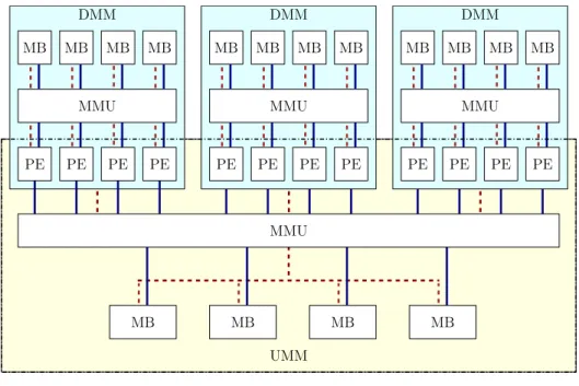
The Discrete Memory Model [61] (DMM) is a simple model designed to capture the essential features of GPU shared memory while the Universal Memory Model [61] (UMM) focuses on the GPU global memory system. Each of these models considers a series of Processing Elements (PEs), a set of Memory Banks (MBs), and a single Memory Management Unit (MMU) that connects them. Figure 3.3 illustrates how the DMM and UMM models view the interconnection between MBs and PEs. The address and data lines between MBs, MMU, and PEs dictate the elements that can be accessed in parallel by the PEs. In the DMM, each MB has its own address and data lines to the MMU, so a single access can be performed on each MB at a time, or else accesses are serialized (i.e., shared memory bank conflicts occur). In the UMM, however, all MBs share an address line to the MMU, so the same address must be accessed from each MB at once (i.e., a coalesced global memory access). The authors present algorithms that perform 2-d array transposition efficiently for the DMM and UMM model [61]. The Hierarchical Memory Model [62] (HMM), illustrated in Figure 3.4, combines the DMM and UMM into a single model of parallel computation that captures the features of both shared and global memory systems of modern GPUs. It models GPU architectures as a single instance of UMM and a series of DMMs, corresponding to the different streaming multiprocessors on modern GPUs.

The SPT model is applied to architectures by selecting a series of operations and estimating overall performance based on the throughput of each operation. However, we do not specify the mechanism used to count the number of each type of operation performed. On modern GPUs, accessing global memory or shared memory are operations that frequently cause performance bot-tlenecks and should therefore by included in the SPT model when applied to GPUs. Thus, existing models of architectures with specific memory systems or optimal access patterns, such as DMM,

(37)

DMM MB MB MB PE PE MB MMU PE PE DMM MB MB MB PE PE MB MMU PE PE DMM MB MB MB PE PE MB MMU PE PE MMU MB MB MB MB UMM

address line data line

Figure 3.4: Illustration of the HMM model that combines several DMMs (shared memory) with a UMM (global memory) into a hierarchy.

UMM, and HMM, are a useful resource that the SPT model can use when analyzing algorithms. We note that, while the DMM, UMM, and HMM models focus on GPU memory systems, in this work we opt to analyze memory accesses using the simpler PRAM and PEM models. In addition to the relative simplicity of the PRAM and PEM models, they allow us to more easily count shared memory and global memory accesses across the entire system, while the DMM, UMM, and HMM only consider accesses performed by a single warp on the GPU, and extending it to the entire system adds complexity.

Model by Kothapalli et al.

The model presented by Kothapalli et al. [48] was one of the first GPU models to attempt to predict overall performance. Similar to our SPT model, they model GPU architectures using a variation of the BSP model [78] by equating individual kernels as supersteps. Within each kernel, they analyze performance by considering only accesses to global memory and shared memory. They provide their own method of analyzing global memory access patterns and use the Read, Queue-Write (QRQW) PRAM [27] model to incorporate the impacts of shared memory bank conflicts. There are, however, several performance factors that they do not consider and that, in this work, we show can have a significant impact on GPU performance: 1) time spent performing register operations, 2) the peak bandwidth of each operation, and 3) instruction-level parallelism (ILP). Thus, the model presented by Kothapalli et al. [48] is a specific instantiation of the SPT model:

(38)

the SPT model instantiated on a GPU architecture with Φ ={φ1 = access global memory, φ2 = access shared memory}, with Mi,I = 1 for all kernels and Bφ1 = Bφ2 = 0. Using the memory models used by Kothapalli et al. [48] to determine A_i,φ₁ and A_i,φ₂ for each kernel K_i of a given algorithm then results in their overall model. Note that this corresponds to the sum variation of their model, as the SPT model computes T as the sum of eachTφ.

Threaded Many-core Model

The Threaded Many-core Model [54] (TMM) considers global memory latency and the impact of multiplicity, along with computation. The TMM has been used to analyze a range of fundamental algorithms [55, 56]: string matching, fast Fourier transform, merge sort, list ranking, and all pairs shortest path. The TMM has been shown to be useful in determining the asymptotic complexity of algorithms on GPUs. As with our SPT model, the TMM incorporates the impact of multiplicity (they refer to asT) on memory access time. However, they ignore the impact of bandwidth, implying that one can continue to reduce the cost of memory access time until you reach the hardware limited number of threads. In Chapter 4, we show that this is not the case and, in fact, one can quickly be limited by bandwidth, even with a relatively small multiplicity. Furthermore, the TMM does not include the cost of synchronization. Rather, they measure algorithm performance by looking at the critical path of execution through the program.

The AGPU Model

The AGPU model, presented by Koike and Sadakane [47] is a thorough GPU-specific performance model that looks at several details of the GPU compute and memory hierarchies. They consider the GPU divided into a series ofmultiprocessors, each withb cores and havingM shared memory. They assume a simplification from the GPU hardware, in that they divide the resources of the GPU into warp-size multiprocessors and do not consider multi-warp thread-blocks. Nevertheless, they present a detailed model that takes into account global and shared memory access patterns and, for a given algorithm, present two asymptotic complexity metrics: the time spent accessing global memory and the time spent accessing shared memory. They also provide a discussion of

multiplicity, which we refer to as oversubscription, though they do not relate it directly to the asymptotic performance of the algorithm. As with the model presented by Kothapalli et al. [48], AGPU can be seen as a specific instantiation of the SPT model that only considers global memory and shared memory as operations. Additionally, the AGPU model only considers the asymptotic performance of algorithms, so, unlike the SPT model, it cannot be used to estimate runtime.

While the AGPU model provides a clear and detailed method of analyzing the asymptotic performance of algorithms on GPUs, it neglects to consider several key factors that we show to have a significant impact on practical performance: 1) time spent performing operations on registers, 2) the interplay between latency, bandwidth, and multiplicity, and 3) synchronization cost. In

(39)

particular, without sufficient multiplicity, practical performance quickly degrades, as we show in Chapter 4. Furthermore, in Chapter 7 we consider the sorting algorithm designed with AGPU [47] and show that insufficient multiplicity causes performance loss. We present a series of improvements to their algorithm and demonstrate a significant performance increase.

Table 3.1: Parameters defined by the hardware system.

Parameter Definition Defined In

U A hardware processing unit Definition 3.1.1

P # of cores inU Definition 3.1.1

Φ Set of operations the system can performs Definition 3.1.1 Lφ Time to perform a single call to operationφ Section 3.1.2 lφ Max. latency ofφ (i.e., whenM= 1) Definition 3.1.9

Bφ Peak bandwidth of φ(i.e., max. number of φper cycle) Definition 3.1.10

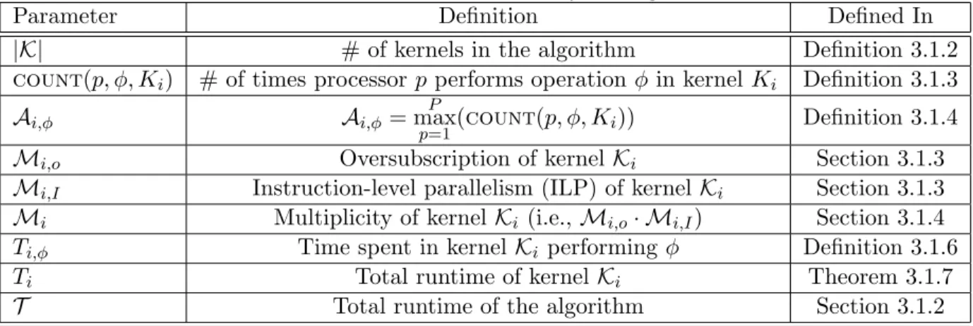
Table 3.2: Parameters defined by the algorithm.

Parameter Definition Defined In

|K| # of kernels in the algorithm Definition 3.1.2 count(p, φ, Ki) # of times processor pperforms operation φin kernelKi Definition 3.1.3

Ai,φ Ai,φ =

P max

p=1(count(p, φ, Ki)) Definition 3.1.4

Mi,o Oversubscription of kernelKi Section 3.1.3

Mi,I Instruction-level parallelism (ILP) of kernel Ki Section 3.1.3

Mi Multiplicity of kernel Ki (i.e.,Mi,o· Mi,I) Section 3.1.4 Ti,φ Time spent in kernel Ki performing φ Definition 3.1.6 Ti Total runtime of kernelKi Theorem 3.1.7

(40)

CHAPTER 4

INSTANTIATING THE MODEL

In this chapter, we consider the features specific to modern GPU architectures to instantiate the SPT model. We first identify operations that we consider the most significant when modeling overall GPU performance. As discussed in Section 1.2, GPU architecture are many-core parallel architectures designed to achieve high computational throughput. Thus, we focus on high latency operations such as accessing slow memory systems or performing synchronization. In particular, for our GPU platforms, we define the set of operations as Φ ={g, s, r, y}, where

• g is accessing global memory,

• sis accessing shared memory,

• r is performing an operation in registers, and

• y is performing intra-thread-block synchronization (i.e.,syncthreads).

Each of these operations has a different corresponding late