Louisiana State University
LSU Digital Commons
LSU Doctoral Dissertations Graduate School
2015
Synthesis With Hypergraphs
Christopher Thomas Alvin
Louisiana State University and Agricultural and Mechanical College
Follow this and additional works at:https://digitalcommons.lsu.edu/gradschool_dissertations Part of theComputer Sciences Commons
This Dissertation is brought to you for free and open access by the Graduate School at LSU Digital Commons. It has been accepted for inclusion in LSU Doctoral Dissertations by an authorized graduate school editor of LSU Digital Commons. For more information, please [email protected].
Recommended Citation
Alvin, Christopher Thomas, "Synthesis With Hypergraphs" (2015).LSU Doctoral Dissertations. 2633.
SYNTHESIS WITH HYPERGRAPHS
A Dissertation
Submitted to the Graduate Faculty of the Louisiana State University and Agricultural and Mechanical College
in partial fulfillment of the requirements for the degree of
Doctor of Philosophy in
The Department of Computer Science
by
Christopher T. Alvin B.A., Ripon College, 1999
M.S., University of Wisconsin at Madison, 2001 M.S., Marquette University, 2011
Acknowledgments
I would like to thank Supratik Mukhopadhyay for his efforts and creativity as my advi-sor. I would also like to thank Louisiana State University and the Economic Development Assistantship. To Sumit Gulwani for his creative ideas in intelligent tutoring. I am in-debted to Rupak Majumdar for a chance walk in the Alps, advice, and tremendous ability to simplify complex notions. I also need to thank Michal Brylinski and Jimmie Lawson for their ideas as well as the Misagh Naderi and Brian Peterson for their collaborations.
Table of Contents
ACKNOWLEDGMENTS . . . ii
ABSTRACT . . . v
CHAPTER 1 INTRODUCTION . . . 1
1.1 Geometry Problem and Solution Synthesis . . . 1
1.2 Molecular Synthesis . . . 2
2 HYPERGRAPHS . . . 4
2.1 Graphs . . . 4
2.2 Synthesis Hypergraph . . . 5
2.3 Hyperpaths and Hyper-Reachability . . . 5
2.4 Sub-Hypergraph Selection through Pebbling . . . 7
3 SYNTHESIS OF GEOMETRY PROOF PROBLEMS AND THEIR SOLUTIONS . . . 9
3.1 Introduction . . . 9
3.2 Informal Theoretical Foundations in Euclidean Geometry . . . 11
3.3 Formal Theoretical Foundations in Euclidean Geometry . . . 15
3.3.1 Geometric Classes . . . 15
3.3.2 Theories and Figures . . . 16
3.3.3 Synthesis Hypergraphs and Problems . . . 20
3.4 Algorithm for Problem Generation . . . 24
3.4.1 Step 1: Hypergraph Construction . . . 25
3.4.2 Step 2: Minimal Assumption Generation . . . 26
3.4.3 Step 3: Strictly Interesting Problem Synthesis . . . 27
3.5 Problem Generation Interface . . . 30
3.5.1 Features of a Geometry Problem . . . 30
3.5.2 Query Interface to Problem Generation . . . 31
3.6 Experimental Results . . . 31
3.6.1 Benchmark . . . 32
3.6.2 Evaluation of Algorithm GenProblem . . . 32
3.6.3 Effectiveness of Our Methodology . . . 36
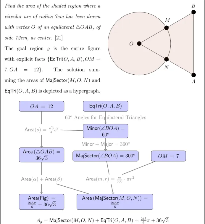
4 SYNTHESIS OF PROBLEMS AND SOLUTIONS FOR SHADED AREA GEOMETRY REASONING . . . 39
4.1 Introduction . . . 39
4.2 Preprocessing: Constructing a Figure of Convex Components . . . 42
4.2.1 Implicit and Computable Properties of a Figure . . . 42
4.2.2 Polygon Identification . . . 45
4.3 Shaded Area Problem Formalization . . . 45
4.4.1 Extending Theories of Figures with Area
Com-putations with a Calculational Logic . . . 49
4.4.2 Synthesis Hypergraph and Problems . . . 51
4.5 Figure Synthesis . . . 54
4.5.1 Figure Synthesis with Templates and Snapping . . . 54
4.5.2 Constraint-Based Synthesis of Problem As-sumptions From a Figure . . . 57
4.6 Solving Shaded Area Problems . . . 59
4.6.1 Atomic Region Identification . . . 59
4.6.2 Constructing the Analysis Hypergraph . . . 63
4.6.3 Finding a Path in the Hypergraph . . . 66
4.7 Problem Generation . . . 67
4.8 Experimental Results . . . 67
4.9 Related Work in Geometry Problem and Solution Synthesis . . . 72
4.9.1 Automated Tutoring Systems . . . 73
4.9.2 Technology for Geometry Education in Proof Synthesis . . . 73
4.9.3 Technology for Geometry Education in Shaded Area Synthesis . . . 74
4.9.4 Automatic Problem Generation . . . 74
5 MOLECULAR SYNTHESIS . . . 76
5.1 Significance of the Problem . . . 76
5.2 Molecular Fragments . . . 80
5.3 Synthesis . . . 83
5.3.1 Algorithms . . . 83
5.3.2 Molecular Filtration with Bloom Filters . . . 87
5.4 Molecular Hypergraph . . . 88
5.4.1 Definitions . . . 88
5.4.2 The Molecular Hypergraph . . . 89
5.5 On-Demand Molecular Hypergraph Construction and Traversal . . . 90
5.6 Experimental Results . . . 92
5.6.1 Self-Reconstruction . . . 92
5.6.2 Cross-Validation . . . 95
5.7 Related Techniques . . . 98
6 CONCLUSIONS AND FUTURE WORK . . . 100
6.1 Generalizing the Hypergraph Approach . . . 100
6.2 Conclusions and Future Work in Geometry Problem Synthesis . . . 100
6.3 Conclusions and Future Work in Molecular Synthesis . . . 102
REFERENCES . . . 103
Abstract
Many problems related to synthesis with intelligent tutoring may be phrased as program synthesis problems using AI-style search and formal reasoning techniques. The first two results in this dissertation focus on problem synthesis as an aspect of intelligent tutoring systems applied to STEM-based education frameworks, specifically high school geometry. Given a geometric figure as input, our technique constructs a hypergraph representing logical deduction of facts, and then traverses the hypergraph to synthesize problems and their corresponding solutions.
Using similar techniques, our third result is focused on exhaustive synthesis of molecules. This synthesis process involves bonding sets of basic, molecular ‘fragments’ according to chemical constraints to create molecules of increasing size. For each input set of fragments, synthesis results in a significant set of molecules. Due to big data constraints we give special consideration in how to construct a corresponding molecular hypergraph based on a target, template molecule. Synthesis of the target molecule in a laboratory environment then corresponds to any path in the molecular hypergraph from the set of fragments to the target molecule.
Chapter 1
Introduction
Program synthesis is the task of automatically discovering an executable piece of code when given constraints through demonstrations, input-output pairs, or other example-based input. Many problems may be phrased as program synthesis problems using AI-style search and formal reasoning techniques; in this dissertation we focus on two distinct synthesis problems. Specifically, we will focus on the construction and exploration of hypergraphs for problem and solution synthesis in intelligent tutoring systems as well as synthesis of molecular compounds. In Chapter 3 and Chapter 4 we describe problem and solution synthesis as applied to STEM-based education frameworks, specifically high-school geom-etry. In Chapter 5, we apply some similar techniques to the space of molecules with the goal of providing the theoretical foundation and toolset for discovery of new antibiotic / antimicrobial compounds.
1.1 Geometry Problem and Solution Synthesis
With the advent of visualization technologies (tablets, graphing calculators, etc.) in the classroom, there has been a shift in mathematics teaching where a problem is viewed from multiple perspectives: graphical, numerical, and algebraic. High school geometry is particularly interesting in this regard because it combines the implicit visual perspective and deductive logic skills. Many online teaching and learning tools exist for high school mathematics courses through Calculus; however there is a limit to the number and types of problems a student may use for practice or a teacher may use for test generation.
On-demand generation of new problems that have specific problem and solution char-acteristics (such as difficulty level, use of a certain set of concepts, etc.) is a difficult task for any teacher. The ultimate goal for problem synthesis is effective student learning, but automating problem synthesis has several benefits including efficient construction of home-work and exams, facilitating effective differentiated instruction, and avoiding copyright issues encountered with textbooks or other copyrighted materials.
In Chapter 3 we present a semi-automated methodology and tool, GeoTutor [7], for generating geometric proof problems of the kind found in a high-school curriculum. We formalize the notion of a geometry proof problem and describe an algorithm for generating such problems over a user-provided figure. Our experimental results indicate that our prob-lem generation algorithm can effectively generate proof probprob-lems in eprob-lementary geometry. On a corpus of 110 figures taken from popular geometry textbooks, our system generated an average of about 443 problems per figure in an average time of 4.7 seconds per figure.
In Chapter 4, we present a tool, GeoShader [8], that not only solves shaded area
ge-ometry problems but also synthesizes such problems. We consider three distinct use cases: 1. given a geometric figure and a shaded region within it, solve the problem by
calcu-lating the area of the shaded region,
2. given a geometric figure, synthesize all possibleinteresting shaded area problems from
it, and
3. given a set of shapes (e.g., triangles, circles, etc.) compose them in all possible configurations (e.g., one shape inside another, one shape adjoining another, etc.) to synthesize a geometric figure that provides interesting shaded area problems.
On a corpus of 102 problems taken from popular geometry textbooks, GeoShader
success-fully solved the original problem and generated an average of 257 problems per figure in an average time of 13.4 seconds per figure. Given a set of three polygons, we synthesized 3533 figures resulting in a mean of 16.5 interesting problems per figure.
1.2 Molecular Synthesis
According to the Centers for Disease Control (CDC), antibiotic / antimicrobial resis-tance is a significant threat that results in at least 23,000 deaths each year [37]. In order to
combat the worldwide epidemic of antimicrobial resistance, we describe a molecular
syn-thesis process that, given a set of basic molecular building blocks (molecular fragments),
constituent molecular fragments. We then discuss validation of our synthesis techniques
and give evidence that our implementation toolSynth is accurate, efficient, and can explore
deep in the chemical compound search space in a short amount of time thus facilitating discovery of new drug compounds.
Chapter 2
Hypergraphs
In each synthesis space we must decide how to encode that information in a target data structure. The synthesis efforts we describe in this thesis generally require deduction of facts. For example, in order to represent logical deduction in a directed graph data structure, we must define correspondences among nodes and edges as well as operations such as paths and reachability. In this section, we first consider a directed graph data structure before expanding into a hypergraph [13], a generalizeation of a graph data structure.
2.1 Graphs
We may define a directed graph based on sets of nodes and edges connecting nodes.
Definition 1 (Directed Graph). A directed graph G(N, E) is a data structure where N
is a set of nodes and E a set of directed edges. Each directed edge e∈E is defined by the
ordered pair e = (s, t) where s, t ∈ N; we may refer to s as the source node and t as the
target node. ∼ = sides ∼ = ∠’s ∼ = sides ∆2 ∆1 ∼ = ∆’s SAS
Figure 2.1: Logical Deduction of Triangle Congruence using SAS
However, for a directed graph G(N, E) where, for all n ∈ N, n corresponds to a
singleton fact, the graph data structure is limiting. General deduction of a single fact often arises from many antecedent facts. For example, as shown in Figure 2.1, the Side-Angle-Side (SAS) geometry congruence axiom requires three facts relating two triangles in order to deduce the single fact that the two triangles are congruent. Our synthesis efforts hence require a more general, many-to-one relationship among facts; thus we require a hypergraph structure.
. . . ◦ . . .
Figure 2.2: A Many-To-Many Directed Hyperedge.
2.2 Synthesis Hypergraph
We first consider a many-to-many hypergraph structure in Definition 2 before focusing on a special case of a hypergraph we use in our synthesis efforts in Definition 3.
Definition 2 (General, Directed Hypergraph). A directed hypergraph (N, E) is a data
structure where N is a set of hypernodes and E a set of directed hyperedges. Each directed
hyperedge e∈E is defined by the ordered pair e= (S, T) where S, T ⊆N.
In a deductive domain, it is not necessary to adopt a many-to-many directed hyperedge as defined in Definition 2 and shown in Figure 2.2. We instead use a hypergraph in which hyperedges consist of many source nodes and a single target node as shown in Figure 2.1 and defined in Definition 3.
Definition 3 (Synthesis Hypergraph). A synthesis hypergraph is a directed hypergraph
H(N, EA) where N is a set of hypernodes and E a set of directed hyperedges over a set
of annotations A. Each directed hyperedge e ∈ E is defined by the ordered pair e = (S, t)
where S ⊆N and t∈N.
2.3 Hyperpaths and Hyper-Reachability
In each of our synthesis efforts, we seek correspondence with the nodes and hyperedges of our synthesis hypergraph as well as operations on those hypergraphs. Specifically, we are most interested in hyperpaths and hyper-reachability. For completeness purposes, we define these concepts with respect to a synthesis hypergraph in Definition 6 and Definition 7, but first we define the necessary structures to acquire hyperpaths.
To simplify this path-finding process we define a ‘reverse’ structure of a synthesis hypergraph by first defining a transpose hyperedge (Definition 4) and secondly the dual of a synthesis hypergraph (Definition 5). We note that the dual of a synthesis hypergraph is a directed graph as stated in Definition 1 where operations on graphs such as path and reachability are well-defined [26].
Definition 4 (Transpose Hyperedge). For a hyperedge e= (S, t) with source nodes S and
target node t, the corresponding transpose hyperedge is a set of edges given byeT ={(t, s) :
∀s∈S}.
Definition 5 (Synthesis Hypergraph Dual). Let H(N, EA) be a synthesis hypergraph with
nodesN and hyperedgesE over a set of annotationsA. The dual of an analysis hypergraph,
HT(N,E), is a graph with nodes N and edges defined by E = S
e∈Ee
T, the union of all
transpose hyperedges of E.
In simple terms, the dual of a synthesis hypergraph is a graph with the same set of nodes and the hyperedges of the hypergraph are split into one-to-one edges with the directions reversed. We may now easily define a hyperpath in a synthesis hypergraph using the dual of a synthesis hypergraph.
Definition 6 (Hyperpath). Let H(N, EA) be a synthesis hypergraph, I ⊂N, and g ∈N.
The hyperpath from I to g is the set of hypernodes and hyperedges corresponding to the
nodes and edges of the path from gto eachf ∈Iin HT. We say that the shortest hyperpath
from I to g is the hyperpath that uses the fewest number of hyperedges.
We can now easily define hyper-reachability in a synthesis hypergraph.
Definition 7 (Hyper-Reachability). Let H(N, EA) be a synthesis hypergraph, I ⊂N, and
g ∈N. Then g is hyper-reachable from I if there exists a hyperpath from I to g.
Both of these operations will play a critical role in each of our forthcoming results in Chapter 3 through Chapter 5.
2.4 Sub-Hypergraph Selection through Pebbling
In a synthesis hypergraphH(N, EA) each hyperedge is annotated with a parameterized
set of valuesA∈ Adefined in the synthesis space. Edge annotations provides the user with
an ability to exclude a set of hyperedges and restrict the corresponding set of syntheses in the synthesis space. We more formally define this notion in a pebbled synthesis hypergraph
in Definition 8 as computed using Algorithm 2.1, a process we informally call pebbling.
Algorithm 2.1 Sub-Hypergraph Selection Through Pebbling
1: procedure Pebble(Hypergraph H(N, EA),NP ⊆N, AP ⊆ A)
2: Hypergraph P . Pebbled Sub-Hypergraph
3: Worklist W ←NP
4: while !W.empty() do
5: n←W.dequeue() . Acquire a node
6: if !n.pebbled() then
7: n.pebble() . Mark the node
8: P.AddN ode(n)
9: for all e∈n.edges do
10: .Consider only allowable hyperedges
11: if e.annotation∈ AP then
12: . If all hyperedge source nodes are pebbled, add target to worklist
13: .to propogate forward 14: if e.pebbled() then 15: P.AddHyperedge(e) 16: W.enqueue(e.target) 17: end if 18: end if 19: end for 20: end if 21: end while 22: return P 23: end procedure
Definition 8 (Pebbled Synthesis Hypergraph). Let H(N, EA) be a synthesis hypergraph
withNP ⊆N a subset of nodes and a subset of annotationsAP ⊆ A. ThenHP (NP, EAP)is
a pebbled synthesis hypergraphcontaining only reachable nodes and hyperedges as dictated
Algorithm 2.1 is a modification of the classic algorithm marking algorithm as first defined by Dowling and Gallier [32] for satisfiability of propositional horn clauses. Pebbling is a linear-time traversal over a synthesis hypergraph that identifies the sub-hypergraph [13] that satisfies the constraints stated by the user. As described in Algorithm 2.1, pebbling is a breadth-first traversal over a synthesis hypergraph where we mark each node with a pebble once it is visited (Line 7). Then on Line 9 through Line 19 we use the following rule for pebbling and propogation: if all source nodes of a hyperedge are pebbled, we place the target node of the hyperedge in the work list. As pebbling continues, we add all pebbled nodes (Line 8) and hyperedges (Line 15) to the sub-hypergraph in preparation for the return of the pebbled version of the hypergraph (Line 22).
Chapter 3
Synthesis of Geometry Proof Problems and Their Solutions
This chapter presents a semi-automated methodology for generating geometric proof problems of the kind found in a high-school curriculum. We formalize the notion of a geometry proof problem and describe an algorithm for generating such problems over a user-provided figure. Our experimental results indicate that our problem generation algorithm can effectively generate proof problems in elementary geometry. On a corpus of 110 figures taken from popular geometry textbooks, our system generated an average of about 443 problems per figure in an average time of 4.7 seconds per figure.
3.1 Introduction
Learning in mathematics is more deeply rooted when a student is able to view a prob-lem from multiple perspectives: graphically, numerically, and algebraically. High school geometry is particularly interesting in this regard because it combines the implicit visual perspective and deductive logic skills. For some, geometry is the favorite mathematics course in high school because of the combination of the implicit visual perspective and the constant exercising of deductive logic skills. This chapter presents a technology to enhance geometry education. In particular, we present a technique for automatically generating fresh geometry proof problems from the figures of given problems.
Generating fresh problems that have specific solution characteristics (such as difficulty level, use of a certain set of concepts) is a difficult task for educators. Automating problem generation has several benefits. First, it can help avoid copyright issues. It is illegal to make photocopies of a textbook and may not be legal to publish an original problem from a textbook on a course website. A problem generation tool can provide instructors with fresh problems (that have characteristics similar to that of the original problem) for use in their assignments, exams, or lecture notes. Second, it can help prevent cheating in classrooms or online education platforms (with unsynchronized instruction) since each student can be provided with a different problem but with the same characteristics. Third, it can be used
to generate personalized workflows for students. If a student solves a problem correctly, then the student may be presented with a problem that is more difficult than the last problem, or exercises a richer set of concepts. If a student fails to solve a problem, then the student may be presented with simpler problems to identify, reinforce, and master core concepts.
We formalize the notion of a geometry proof problem, which consists of a figure, some assumptions about the figure, goals that need to be established about the figure, and the set of axioms that need to be used. We propose a semi-automated methodology for generating such problems. Given a figure and a set of axioms, our problem generation technique produces a set of problems over that figure in the form of pairs of assumptions and goals. Such problems, generated across a large set of figures provided by the user, can be stored in a database along with their characteristics. This empowers users to query the database with specific characteristics to obtain custom problems.
Our problem generation technique operates in three steps. First, it produces a logi-cal geometry hypergraph (Definition 14) that represents all possible proofs for all possible problems over a given pair of user-provided figures and axioms. The hypergraph construc-tion requires enumerating all facts that are true of the figure as nodes in the hypergraph. Furthermore, a set of source facts is connected to a target fact using a directed hyperedge labeled with a user-provided axiom if the axiom can be used to deduce the target fact from the source facts. Then, the tool systematically enumerates all minimal sets of assumptions (Algorithm 3.1). An assumption is a fact about the figure, and informally, a set of as-sumptions is minimal if every assumption is non-redundant. Finally, for any minimal set of
assumptions I, the tool systematically enumerates all possible goal setsG such that (I, G)
is an interesting problem (Algorithm 3.2).
We evaluated the effectiveness of our problem generation algorithm on 110 figures taken from various geometry textbooks. Our algorithm generated an average of 443 problems in
an average time of 4.7 seconds per figure. We also observed that there were several problems with same characteristics across various figures.
This chapter makes the following contributions:
• We informally describe the geometry proof problem synthesis domain (§3.2).
• We then formalize a geometric figure as a partial ordering of geometric classes as well
as the notion of a geometry problem (§3.3).
• We then motivate problem generation interfaces corresponding to characteristics of
geometry proof problems (§3.5).
• We present a technique for generating proof problems over a given geometric figure
(§3.4).
• We describe experimental results illustrating the efficacy of our problem generation
interfaces and our problem generation algorithm (§3.6).
3.2 Informal Theoretical Foundations in Euclidean Geometry
Informally, a geometric figure is a pictorial representation of a collection of geometric objects (points, lines, circles) in a specific orientation with each other. Internally, we repre-sent geometric figures using first-order logic constraints which can be derived by analyzing a pictorial representation. We work in a first order language with arithmetic and constants ranging over points. We omit a full description of the logical language and illustrate it
through examples. Our logic consists of relations such as betweenness Between(A, B, C)
(which implies collinearity of pointsA,B, andC), congruence, and equality relations on line
segments or angles. For ease of readability, in the following examples, we also use derived
predicates such as Triangle(A, B, C) (the three points form a triangle, denoted ∆ABC),
Collinear(A, B, C) (points are collinear), RightAngle(A, B, C), etc.
We compute internal representations from pictorial representations of a figure. We assume that input figures are drawn to scale but the problem instances we generate will not assume that figures are drawn to scale. Thus, in the internal representation for a
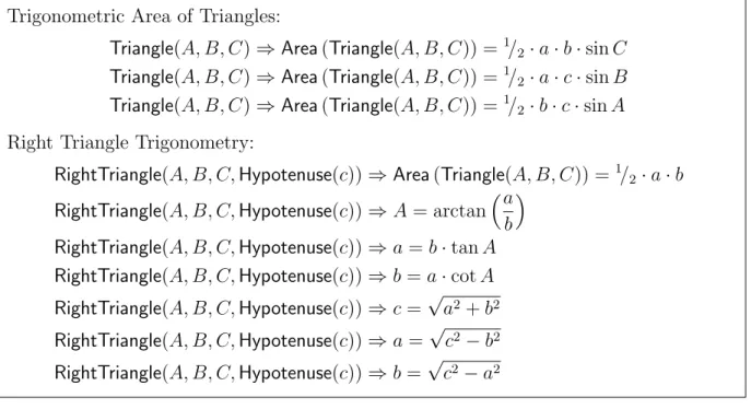
Table 3.1: Example Set of Geometric Axioms
Axiom Name Premise(s) Conclusion(s)
Midpoint Definition Midpoint(M,AB) AM =M B
Angle Addition ∠ABC,∠CBD ∠ABC+∠CBD=∠ABD
Exterior(D,∠ABC)
Vertical Angles Intersect(X, AB, CD) ∠AXD∼=∠CXB,
∠AXC∼=∠BXD
Side-Side-Side ∆ABC,∆DEF, ∆ABC ∼= ∆DEF
AB∼=DE, BC ∼=EF
CA∼=F D
Alternate Interior Angles CDkEF, ∠EN M ∼=∠N M D,
Intersect(M, AB, CD), ∠F N M ∼=∠N M C
Intersect(N, AB, EF)
figure Fig, we distinguish between implicit and explicit facts. Implicit predicates only
provide orientation (or “betweenness”) information but not relationships on measurements. Explicit predicates provide relations based on measurement and may not hold when the
figure is distorted. For example, implicit predicates would state that ABC is a triangle
or that line segments AB and CD intersect at M, and explicit predicates would state
AB =CD or∠ABC is a right angle. Technically, implicit predicates are those facts about
the figure provable inordered geometry[27], and explicit predicates are those facts provable
in Euclidean geometry minus the implicit ones. For a figure Fig, we write I(Fig) for the
set of implicit facts and E(Fig) the set of explicit facts.
We may now formalize the definition of a geometry axiom as a mechanism that uses a set of facts to derive a new target fact.
Definition 9 (Geometry Axiom). A geometry axiom is a Horn clause whose ground
in-stances are implicit or explicit predicates and consists of a set of premisesand a conclusion.
The free variables in a geometry axiom are (implicitly) universally quantified. Given
an axiom A, we say that A derives a predicate p from a set P of predicates if there is an
instantiation of the premises ofA withP and the conclusion withp: P `A
p. Table 3.1 gives some examples of geometry axioms.
Definition 10 (Geometry Problem). Let Figbe a figure, I(Fig)be the set of implicit facts,
and Axm be a set of geometry axioms. A geometry (proof) problem over (Fig,Axm) is a
pair (I, G), where the assumptions I ⊆ E(Fig) and goals G ⊆ E(Fig) are sets of explicit
facts such that I∩G=∅andI(Fig)∪I∪Axmimply each g ∈Gusing first-order reasoning.
In Definition 10 we require the disjointness condition between I and Gto ensure
prob-lems are non-trivial, and the derivation condition to ensure probprob-lems have solutions. Given a geometry problem, we may now define a converse geometry problem.
Definition 11 (Converse Geometry Problem). The converse of a problem (I, G) over
(Fig,Axm) is the problem (G, I) over (Fig,Axm), if it is indeed a problem.
We note that a corresponding converse problem may not exist for a given (I, G) over
(Fig,Axm). We may now define concepts related to the quality of a geometry problem.
Definition 12 (Strict, Interesting Geometry Problem). A geometry problem (I, G) over
(Fig,Axm) is interesting if no strict subset of I together with I(Fig) can establish every
goal in G using Axm. An interesting problem is strict if G is minimal, i.e., (I, G0) is not
interesting for any strict subset G0 (G.
Observe that an interesting problem where G is a singleton is strict.
Definition 13 (Complete Geometry Problem). An interesting geometry problem (I, G)
over (Fig,Axm) is complete if for any predicate p∈ E(Fig), I(Fig)∪I ∪Axm derives p.
A complete problem is strict if it is not complete for any strict subsetG0 ofG. Figure 3.1 gives some examples of interesting and complete geometry problems.
Let (I, G) be a problem over (Fig,Axm). A proof that I(Fig)∪Axm∪I derives G
consists of first-order derivations, one for each g ∈G, whose root is labeledg, whose leaves
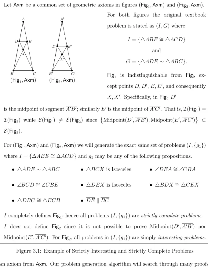
Let Axmbe a common set of geometric axioms in figures (Fig1,Axm) and (Fig2,Axm). B A C D E X (Fig1,Axm) B0 A0 C0 D0 E0 X0 (Fig2,Axm)
For both figures the original textbook
problem is stated as (I, G) where
I ={4ABE ∼=4ACD}
and
G={4ADE ∼ 4ABC}.
Fig1 is indistinguishable from Fig2
ex-cept points D, D0,E, E0, and consequently
X, X0. Specifically, in Fig2 D0
is the midpoint of segmentA0B0; similarlyE0 is the midpoint ofA0C0. That is,I(Fig 1) = I(Fig2) while E(Fig1) 6= E(Fig2) since Midpoint(D0, A0B0),Midpoint(E0, A0C0) ⊂ E(Fig2).
For (Fig1,Axm) and (Fig2,Axm) we will generate the exact same set of problems (I,{g1})
where I ={∆ABE ∼= ∆ACD}and g1 may be any of the following propositions.
• 4ADE ∼ 4ABC • ∠BCD∼=∠CBE • 4DBC ∼=4ECB • 4BCX is Isosceles • 4DEX is Isosceles • DE kBC • ∠DEA∼=∠CBA • 4BDX ∼=4CEX
I completely defines Fig1; hence all problems (I,{g1}) are strictly complete problems.
I does not define Fig2 since it is not possible to prove Midpoint(D0, A0B0) nor
Midpoint(E0, A0C0). For Fig
2, all problems in (I,{g1}) are simplyinteresting problems.
Figure 3.1: Example of Strictly Interesting and Strictly Complete Problems
an axiom from Axm. Our problem generation algorithm will search through many proofs.
Hence, we use a hypergraph representation for all possible derivations. Since the setI(Fig)
Definition 14(Logical Geometry Hypergraph). For a pair(Fig,Axm), the logical geometry
hypergraph H(Fig,Axm) is a synthesis hypergraph whose nodes consist of all predicates in
E(Fig) and whose edges are of the form (P, p, A), where P ⊆ E(Fig) is a set of explicit
predicates, p ∈ E(Fig) is an explicit predicate, and A ∈ Axm, such that there exists a set
Q⊆ I(Fig) such that A derives p from P ∪Q.
We then say reachability in the logical geometry hypergraph corresponds to logical derivability. For a set T ⊆ E(Fig), we define
Derive(T) = {g ∈ E(Fig)|T ∪ I(Fig)∪Axm|=g}.
The setDerive(T) coincides with the set of nodes reachable in the hypergraphH(Fig,Axm)
starting from the setT of nodes. Thus,Derive(T) can be computed for every setT ⊆ E(Fig)
in time polynomial in the size of the hypergraph.
3.3 Formal Theoretical Foundations in Euclidean Geometry
In this section we consider a more formal discussion of the framework for problem synthesis in Euclidean geometry. In these discussion, we assume immutable figures in which the properties of that figure are not allowed to be modified nor any new information constructed.
3.3.1 Geometric Classes
There are several distinct types of objects in Euclidean geometry, most notably: points, rays, segments, lines, triangles, quadrilaterals, and circles. For our purposes, we define a
class for each geometric object: the class of points P, the class of segments S, the class of
triangles T, etc.
Since points are considered to be the framework for which Euclidean geometry is
founded, the only characteristic we will impose on a point is a coordinate in n
dimen-sions (n ≥2); that is, we coordinatize our geometry even if it is not apparent to the user.
This also implies coordinate axes for the user interface even though they may be trans-parent to the user. As our focus is high school Euclidean geometry, we will restrict our
notion of a point to two or three dimensions as needed. We define the class of segments
in terms of the class of points. We define the class of all triangles T as a collection of sets
of three segments with the constraint that their intersections result in three unique points: the vertices of a triangle.
3.3.2 Theories and Figures
LetLbe a logic [22] in which properties of a geometric figure are described. We assume
a finite set of geometric classes including point, segment, triangle, isosceles triangle, and equilateral triangle. Let Fig = {Fig1, . . . ,Figk} be the collection of k geometric classes.
Also let Fig be a figure that belongs to a class Fig: formally, Fig ∈ Fig. We then define
the theory of a class of figures Fig as Th(Fig) = {φ1, . . . , φj} where each φi is a property
(a formula in L) and 1 ≤ i ≤ j enumerate the minimal set of the implicit properties of
Fig, I(Fig); i.e., ∀φi ∈ Th(Fig),{Th(Axm)∪Th(Fig)\φi} 2 φi where Axm is the set of
Euclid’s axioms [51]. That is, Th(Fig) consists of all properties of a class Fig that are
innate to the class, but cannot be proven; in other words, implicit properties are those provable in ordered geometry [27]. For example, in the triangle class, one can neither prove that triangles have three segments nor prove that they have three internal angles. These are the implicit properties of the triangle class.
Ordering on Geometric Classes. The geometric classes defined in§3.3.1 give rise to an
ordering among particular sets of classes. We first define the ordering operator and then prove that it implies a partial order on the set of geometric classes.
Definition 15 (Class Ordering Operatorv). We define the ordering operator von classes
as Fig1 v Fig2 if and only if Th(Fig1) Th(Fig2), i.e., if Th(Fig1) logically entails
Th(Fig2).
Proposition 1 (Partial Order of v). v defines a partial order on Fig.
Proof. Let Figc ∈ Fig. Then it is clear Th(Figc) Th(Figc). Hence, v is reflexive. Let
Th(Fig2)Th(Fig1). This implies that for the logical formulae p1, . . . , pk∈Th(Fig1) and
q1, . . . , q` ∈Th(Fig2),∀qi,∃{pj}qi and similarly∀pi,∃{qj}pi. This impliesFig1 =Fig2
and thus v is antisymmetric.
Let Fig1,Fig2,Fig3 ∈ Fig with Fig1 v Fig2 and Fig2 v Fig3. By definition, Th(Fig1)
Th(Fig2) andTh(Fig2)Th(Fig3). Since theories are logical formulae, it follows thatFig1
is the set of logical formulae such that Th(Fig1)Th(Fig3). Hence, Fig1 v Fig3 and v is
transitive.
For a figure Fig to be described by a particular class Fig we say that the figure forces
the theory of the classFig: FigTh(Fig). ThusFig∈Figif and only ifFigTh(Fig). We
now need to show that a figure cannot be an element in two distinct chains in the partial order; e.g. a figure cannot be both a triangle and circle.
Lemma 3.3.1 (Unique Figure Chain). For a figure Fig and classes Fig1 and Fig2, if Fig∈
Fig1 and Fig∈Fig2, then either Fig1 vFig2 or Fig2 vFig1.
Proof. Suppose without loss of generality Fig1 6 vFig2. By definition, Fig Th(Fig1)
and Fig Th(Fig2). As Fig1 6 vFig2, there exists a logical formula p ∈ Fig2 such that
Fig Th(Fig1) 2 p. As Fig Th(Fig2) p, this is a contradiction so Fig1 v Fig2 as
desired.
We also require a figure to be defined by the most appropriate class.
Corollary 3.3.2. For a figure Fig, there exists classes Figb and FigB such that for Fig ∈
Figb,Fig ∈FigB and for all Fig0 such that Fig∈Fig0, Figb vFig0 vFigB.
Figbdefines the greatest lower bound of classes for a figureFig. We callFigbthestrongest
class corresponding to figureFig and writestrong(Fig). FigB defines the least upper bound
of classes for a figure Fig. We call FigB the weakest class corresponding to figure F and
write weak(Fig). As an example, consider the class of triangles (T), isosceles triangles (I),
and equilateral triangles (E), it is clear E v I v T asE contains the most information and
A B C D E F A0 B0 C0 E0 D0 F0 Figure 3.2: Invariant FiguresFig and Fig0 (Fig≈Fig0)
Given a geometric figure Fig, we will construct two sets of properties that describe
Fig. The first set of properties, I(Fig), describe the invariant characteristics of Fig. That
is, we note the relationships among the points, lines, and shapes that are independent of
specific information about Fig; that is, angles and distances between points may differ but
not the overall structure of the figures as previously described in §3.2 according to ordered
geometry [27]. In Figure 3.2 two distinct figuresFigandFig0 are invariant. We now formally
define the notion of invariance between figures.
Definition 16 (Invariant Figures). Two figures G and G0 are invariant if there exists a
class of geometric figures Fig such that weak(G) =Fig =weak(G0). We write G≈Fig G0
to say figure G is invariant to figure G0 with respect to class Fig.
For a figure Fig, we define the theory of Fig denoted by Th(Fig) to be Th(Fig) where
Fig = strong(Fig). We may also extend to the theory of a class Fig being defined as all
figures in Fig implying all properties of Fig.
As an example, let figureFigbe a right triangle4ABC withm∠BAC = 90o (m∠BAC
refers to the measure of ∠BAC). The theory of Fig, denoted byTh(Fig) is given by
Th(Fig) = {4ABC, m∠BAC = 90o}={Triangle(A, B, C),RightTriangle(B, A, C)}.
Let T be the class of triangles and Tr be the class of right triangles, then we note for
the right triangle F above, it is true that F ∈ T and F ∈ Tr with Tr v T.
Geometric Axioms. For Euclidean geometry, we assume modified versions of Euclid’s original axioms [51]; these axioms are universally quantified. These axioms are stated below:
1. Segment Addition: If B is betweenA and C, then AB+BC =AC.
2. Angle Addition: If pointDlies on the interior of∠ABC, thenm∠ABD+m∠DBC =
m∠ABC.
3. Angle Addition for Straight Angles: If∠ABC is a straight angle and D is any point
not on
←→
AC, then m∠ABD+m∠DBC+m∠ABC = 180o.
4. Algebraic Properties of equality including addition, subtraction, multiplication, and division.
5. Equality (=). congruence (∼=), and similarity (∼) are equivalence relations.
The set of axioms describing algebraic properties of equality including addition, sub-traction, multiplication, and division and those describing the fact that equality (=).
con-gruence (∼=), and similarity (∼) are equivalence relations are called the algebraic axioms
and are denoted by Axma. In addition, a few existentially quantified axioms are assumed:
1. A line contains at least two points.
2. Through any two points, there exists exactly one line.
3. If two parallel lines are cut by a transversal, then corresponding angles are congruent. 4. SSS, SAS, and ASA congruency of triangles.
5. Corresponding Parts of Congruent Triangles are Congruent (CPCTC). 6. AA Similarity of Triangles.
Each of the axioms above requires an encoding into a logical form. For the Segment Addition Axiom to be applied, we require two distinct pieces of information: (1) three points are collinear, (2) which of the three points lies between the other two points. Consider a
segment χ1χ2 with point χ3 between χ1 and χ2. Then
With CPCTC, we require two congruent triangles and the labeling of the respective vertices of the congruent triangles to be consistent:
(∆ABC)∧(∆DEF)∧(∆ABC ∼= ∆DEF)⇒(AB∼=DE)∧(∠ABC ∼=∠DEF)∧
(CA∼=F D)∧(∠BCA ∼=∠EF D)∧
(BC ∼=EF)∧(∠CAB ∼=∠F DE)
Definitions of Geometric Terms. We presume standard definitions of common
geomet-ric terms; e.g.:
• Collinear refers to a set of points lying on one line.
• Midpoint of a segment refers to the point that divides a given segment into two
congruent segments.
These definitions have ramifications because they imply more properties regarding a
figure. For example, if M is the midpoint of XY, then the definition states XM =M Y.
However, the definitions are implicit in the theory of a figure F as well as the theory of
given information. For a figure Fig, we call this information the theory of assumptions,
Th IFig
.
3.3.3 Synthesis Hypergraphs and Problems
The formal framework we use to represent a geometric figure together with the assump-tions is a hypergraph. Proof problems will be synthesized by exploring this hypergraph. Given only a figure, we may construct a corresponding hypergraph based solely on the implicit properties, axioms, and student knowledge base. The student knowledge base comprises the lemmas and theorems that the student possesses in their knowledge base.
Definition 17 (Basic Geometry Synthesis Hypergraph). Given a figure Fig, the basic
geometry synthesis hypergraph corresponding to Fig is HbFig(P, E) where P is the set of
nodes and E is the set of hyperedges. We define the set of nodes in the hypergraph P =
and Axmx is the set of Euclid’s axioms. The hyperedges E of the hypergraph are defined
as a set of functions mapping a set of nodes to a single node: E ⊆
|P|
[
i=1
Pi → P where
hp1, . . . , p`i →p∈E if Th(Fig)∪Th(Axmx)|=p1∧. . .∧p` ⇒p holds true.
Each node in the basic hypergraph is typed so it belongs to one discrete class in the
set of types τ ={algebraic, geometric}. We make these distinctions among nodes so that
later we may formally define a problem with respect to a basic geometry hypergraph. We now define how the type of each node in a basic geometry hypergraph is acquired.
Definition 18 (Algebraic and Geometric Nodes). Let n be a node in a basic geometry
synthesis hypergraph H. If n is a propositional formula associated with some a∈Axma, we
say n is a purely algebraic node. We define leaves HT to be the set of all nodes in HT
without parents. If for all `∈leaves HT such that there exists a path from n to ` in HT,
` is a purely algebraic node, we say n is an algebraic node. We note that purely algebraic
nodes are considered algebraic nodes. We similarly define the terms purely geometric nodes
and geometric nodes for Euclid’s axioms, Ax.
We can extend our notion of the basic geometry hypergraph HbFig for a geometric
figure Fig by including the problem statement in the corresponding hypergraph. This is
accomplished by incorporating the assumptions, IFig, and the goal, g.
Definition 19 (Standard Geometry Synthesis Hypergraph). Given a figure Fig and
corre-sponding basic geometry synthesis hypergraph, HbFig(P, E), the standard geometry
syn-thesis hypergraph corresponding to Fig with assumptions IFig and goal g, is given by
HFig
s HbF, Pg, Eg, g
. We define the additional set of typed nodes in the hypergraph Pg =
Th IFig
∪ {g}. The corresponding additional hyperedges, Eg are a result of the theories
derived from all typed nodes given by P ∪Pg where P are the typed nodes defined in H
Fig b . It is clear that for a figure Fig, HbFig is a sub-hypergraph [13] of HFig
s .
If we do not distinguish between a basic hypergraph or standard hypergraph we will
P is the set of typed nodes and E is the set of hyperedges. We note that this definition is analogous to the logical geometry hypergraph of Definition 14.
Geometry Problems. Now that we have defined a hypergraph in the deductive space
of Euclidean geometry, we can define a geometry problem with respect to problem hyper-graphs. A traditional high school geometry problem in simplest form is a natural language statement, but more common is the combination of a description composed of mathemati-cal relationships and natural language which describe a figure. In a problem hypergraph, we informally define a problem as a set of typed nodes that describe the assumptions of the problem and a corresponding typed goal node that follows from the assumptions. The corresponding path from the typed assumption nodes to the typed goal node is a solution to the problem (i.e., a proof of the goal).
Definition 20 (Basic and Standard Problems). Given a basic hypergraphHbFig
correspond-ing to a figure Fig, a basic geometry problemP is a statement of the formp1∧. . .∧pk`p
for some k > 0 where for all i, pi is the propositional formula corresponding to typed node
ni of H Fig
b , p is the propositional formula corresponding to typed node n of H
Fig
b , and there
exists a path P from hn1, . . . , nki to n. The path P is a solution to geometry problem P.
For a node g, we say that Pg defines the collection of all paths in hypergraph HbFig with
goal node g; a valid student solution is any path in Pg. A standard geometry problem is
defined similarly for a standard hypergraph HFig
s .
We will use the general termproblem in situations where the context is clear. For a goal
g and a set of source nodesSin a standard hypergraphHsFig
HbFig, Pg, Eg, g
corresponding
to figure Fig with assumptions A, we say that S is strict with respect to g if S ` g is a
problem and no U `g is a problem forU ⊂S as stated in Definition 12.
As mentioned in§3.1, not all problems are interesting. Interesting problems for a figure
and a set of assumptions are those that require at least one or more of the assumptions, the assumptions are minimal with respect to the goal, and the goal cannot be derived from a set of algebraic expressions through purely algebraic manipulation.
Analogous Problems. We use the termanalogousto define a problem as an independent, ’interesting’ problem that mimics the difficulty and length of a given problem. For a
prob-lem P in a hypergraphH, the problem hypergraph ˜P is the sub-hypergraph of H induced
by P. We begin with a strict view of problem analogy that views problem hypergraphs as
graphs.
Definition 21 (Coarse Problem Homomorphism). LetH(V, E)andH0(V0, E0)be problem
hypergraphs. Thenφ:H →H0 is a coarse problem homomorphismifvi ∈V for1≤i≤k,
for all hv1, . . . , vki=~v ∈P(V) such that (~v →v)∈E for v ∈V,
• v and φ(v) are typed nodes in which type(v) = type(φ(v))∈τ ,
• ~v and φ(~v) are sets of typed nodes in which |~v|t=|φ(~v)|t for each type t∈τ, and
• there exists an edge φ(~v)→φ({v})∈E0.
In Definition 21 we define analogous problems by requiring (1) corresponding node types be equivalent for each problem, (2) for each corresponding edge the number of source nodes of each type are equivalent and the the target node of the edge is of the same type, and (3) each edge has a corresponding edge in both problems. We may now define a coarse problem isomorphism based on the structural requirements of the coarse problem homomorphism.
Definition 22(Coarse Problem Isomorphism). φis a coarse problem isomorphismif (i)φ
is a bijection, (ii) φ is a coarse problem homomorphism, and (iii) φ−1 is a coarse problem
homomorphism. If φ is a coarse problem isomorphism between H and H0, we may write
H ∼=cH0.
Definition 23 (Coarsely Analogous Problem). Two problems P1 andP2 are coarsely
anal-ogous if there exists a coarse problem isomorphism between P˜1 and P˜2.
In Figure 3.3, the two problems proving that (F) ∆BM C is isosceles and (G) ∆DM A
In the figure at right, assume
1. M is the midpoint of AC,
2. M is the midpoint of BD, and
3. m∠BCD= 90o.[75]
A
D C
B
M
With the given set of assumptions using the associated figure, we may prove the fol-lowing set of facts.
(A) ∆BM C ∼= ∆DM A, (B) m∠ADC = 90o, (C) ∆ADC ∼= ∆BCD, (D) 2BM =AC, (E) ∆DM C is isosceles, (F) ∆BM C is isosceles, (G) ∆DM A is isosceles, (H) BC k AD. (BC is parallel to AD.)
Figure 3.3: Provable Facts From A Geometric Problem Statement
to formally capture the notion of “analogy”. For example, in Figure 3.3 a student who has been able to prove statements (F) and (G) should also be able to prove statement (E) since all three statements require one to prove that a particular triangle is isosceles although the task of proving (E) is not coarsely analogous to that of proving (F) nor (G).
Formally capturing a weaker notion of analogy motivates the following definition.
Definition 24 (Goal Analogous Problems). Let P1 and P2 be two problems with goals g1
andg2, respectively. We say problemsP1 andP2 are goal analogous problemsif type(g1) =
type(g2) and strong(g1) =strong(g2). This is clearly an equivalence relation and we refer
to the induced equivalence classes as a goal analogous partition.
3.4 Algorithm for Problem Generation
Our algorithm for problem generation has three steps. The first step creates a hyper-graph according to Definition 14 that represents all possible proofs for all possible problems over a given pair of a user-provided figure and axioms. The second step systematically enu-merates all minimal sets of assumptions (Algorithm 3.1). The third step enuenu-merates, for
Using the provided figure and the fact
that M is the midpoint of AB, prove that
2AM =AB and 2M B =AB. A(0,0)
B (2,0)
M
(4,0)
Figure 3.4: Statement of the Midpoint Theorem
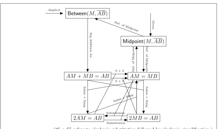
Implicit Giv en Between(M, AB) Midpoint(M, AB) Seg Addition Ax Def. of Midp oin t Def. of Midp oin t AM +M B =AB Subst + Simp S + S S + S AM =M B Subst + Simp Def. of Midp oin t 2AM =AB Subst + Simp 2M B =AB Substitution Substitution
(“S + S” refers to algebraic substitution followed by algebraic simplification.)
Figure 3.5: Logical Geometry Hypergraph for the Midpoint Theorem of Figure 3.4 interesting problem.
In the following exposition, we focus on clarity rather than performance. The
enumer-ation of problems is exponential in the worst case; we show in §3.6 that nevertheless, the
enumeration can be performed successfully in practice.
3.4.1 Step 1: Hypergraph Construction
We compute a logical geometry hypergraph as defined in Definition 14. The input
to the algorithm is a geometry figure Fig drawn to scale and a set of axioms represented
as Horn clauses. The algorithm internally computes the sets I(Fig) and E(Fig) and then
Algorithm 3.1 Algorithm AllMinimalSets
1: Input: Figure Fig, axioms Axm
2: Output: Set of all minimal sets of E(Fig)
3: AllSets ← {∅}
4: Old ← ∅
5: while AllSets 6=Old do
6: Old ←AllSets
7: for all I ∈AllSets do
8: for all f ∈ E(Fig) s.t. Derive(I)6=Derive(I∪ {f}) do
9: AllSets ←AllSets ∪ {I∪ {f}}
10: end for
11: end for
12: end while return AllSets
compute Derive(T) queries for sets T ⊆ E(Fig) in the subsequent steps of the algorithm.
As an example, we consider the Midpoint Theorem, often the first proof in a geometry course, as stated in Figure 3.4. We note that the statement of the Midpoint Theorem has I ={Midpoint(M, AB)} and G={2AM =AB,2M B =AB} with |G|= 2. We also note that the figure associated with the problem in Figure 3.4 provides a set of sample coordi-nates demonstrating the embedding of the figure in the Euclidean plane thus facilitating computation of the geometric facts of I(Fig) andE(Fig).
We then construct the logical geometry hypergraph corresponding to the problem in Figure 3.4 in Figure 3.5. In this construction of the hypergraph for Figure 3.4, the geometry
facts describing each node are self-explanatory except for Between(M, AB). The Between
predicate construct (1) implies collinearity of the three points M,A, andB and (2)M falls
between the endpoints of the segment A and B. In other words, for M 6=A and M 6=B,
Between(M, AB) ⇐⇒ AM +M B =AB.
3.4.2 Step 2: Minimal Assumption Generation
A set T ⊆ E(Fig) is minimal if either T = ∅ or for each t ∈ T, we have that T \ {t}
is minimal and Derive(T) 6= Derive(T \ {t}). Minimality is a necessary condition for an
Algorithm 3.2 Algorithm GenProblem
1: Input: FigureFig, axioms Axm, minimal set I ⊆ E(Fig)
2: Output: Strictly interesting problem (I, G)
3: G =∅ 4: while ∃f ∈I s.t. G⊆Derive(I\ {f})do 5: f =choose({f ∈I |G⊆Derive(I \ {f})}) 6: T = Derive(I)\Derive(I\ {f}) 7: g = choose(T \I) 8: G = G∪ {g} 9: end while 10: return (I, G)
In the second step, the problem synthesis algorithm systematically enumerates all min-imal sets of assumptions; Algorithm 3.1 is a simple fixed-point procedure to compute the set of all minimal sets.
Theorem 3.4.1 (Completeness ofAllMinimalSets). AllMinimalSets(Fig,Axm)returns the
set of all minimal sets for a pair (Fig,Axm), .
Proof. As a base case, consider a singleton fact p∈ E(Fig) that defines a minimal set{p}.
On Line 3,AllSets ={∅}. Therefore, the first time through the generative loop from Line 8
through Line 10, I =∅. Hence, for p∈ E(Fig), since {p} is a minimal set, ∅ ∪ {p}={p}is
added to AllSets on Line 9 and is thus generated by AllMinimalSets.
Suppose M = {p1, . . . , pk} is a minimal set containing k > 1 facts generated by
AllMinimalSets. Also suppose for some q ∈ E(Fig), M ∪ {q} is a minimal set. As M
is a minimal set, M ∈ AllSets. Hence, at some point during execution, I = M (Line 7).
Sinceq∈ E(Fig) andM∪{q}is a minimal set containingk+ 1 facts satisfying the condition
on Line 8, it follows M∪ {q} ∈AllSets (Line 9).
3.4.3 Step 3: Strictly Interesting Problem Synthesis
The final step enumerates, for each minimal set of assumptionsI, all possible goal sets
We present the third step as the non-deterministic procedure in Algorithm 3.2. It takes
as input a figure Fig and axioms Axm, as well as a minimal set I of explicit predicates. It
computes a strictly interesting problem by “growing” a set G of goals and returns (I, G)
as the generated problem. Initially, the set G is empty (Line 3). While the current set
of goals is not strong enough to ensure the problem is interesting (Line 4), the algorithm generates a new goal. To generate a new goal, the algorithm finds (non-deterministically,
Line 5) an assumption f that is not used to prove the current set of goals and finds
(non-deterministically, Line 6) a goal that is derivable using I but not without this assumption.
Notice that since I is minimal, the set T on Line 6 is non-empty. However, to ensure the
condition I∩G=∅, we choose g from the set T \I on Line 7, which may be empty.
By construction, Algorithm 3.2 ensures that returned problems are strictly interesting.
For the returned pair (I, G), since the while loop exits, we know that every f ∈ I is
necessary to prove some goal in G; hence (I, G) is interesting. Further, the problem is
strictly interesting since the algorithm returns a minimal set of goals G.
The non-deterministic choices of the algorithm are denoted by the choose operator,
which selects an element of a set (if non-empty), and fails otherwise. By iterating over pos-sible non-deterministic choice, the algorithm can generate every pospos-sible strictly interesting
problem with assumption I.
Finally, in order to generate a complete problem, we can check that the input I to
procedure GenProblem can derive all explicit facts, i.e., Derive(I) = E(Fig).
Theorem 3.4.2 (Soundness of GenProblem). If GenProblem(Fig,Axm, I) returns (I, G)
for a minimal set I, then (I, G) is a strictly interesting problem over(Fig,Axm).
Proof. Suppose GenProblem returns (I, G) where G = {g1}. In this base case it is clear
that executing GenProblem on Line 3 that ∅ ⊂ G. (I,∅) is clearly not an interesting
problem and the loop (Line 4 to Line 9) will be executed. With a choice of g1 (Line 7)
GenProblem will generate (I,{g1}). It follows that (I,{g1}) is strictly interesting since the
Now supposeGenProblem returns (I, G) where G={g1, . . . , gk} fork >1. Take some
g ∈ G. During execution, the loop condition (Line 4) in GenProblem would be satisfied
for G \ {g}; thus (I, G \ {g}) would not be returned as a strictly interesting problem.
That is, there exists f ∈I such that G\ {g} ⊆Derive(I\ {f}). Specifically, for all subsets
G0 =G\{g}whereg is an arbitrary element ofG,GenProblemwould continue to loop since
(I, G0) is not an interesting problem. The final loop execution would non-deterministically
choose g (Line 7) to construct the original set G = G0 ∪ {g} = {g1, . . . , gk} for k >1. It follows (I, G) is a strictly interesting problem.
Theorem 3.4.3 (Completeness of GenProblem). If (I, G)is a strictly interesting problem
for (Fig,Axm), there is a run of GenProblem(Fig,Axm, I) that returns (I, G).
Proof. Suppose (I, G) is a strictly interesting problem for (Fig,Axm) whereG={g1, . . . , gk}
for k ≥1. We will construct a set of G0 from∅ untilG0 =G at the end of the run.
In the first execution of the loop, we have for all f ∈ I, ∅ = G0 ⊆ Derive(I \ {f}).
We choose some f and subsequently some gc ∈ Derive(I)\Derive(I\ {f})\I (Line 7).
We note that many facts may exist in Derive(I)\Derive(I \ {f})\I; however, we
non-determindistically choose a desired goal in the G: gc ∈ G. PutG0 = {gc}. Since (I, G) is
strictly interesting, (I, G0) is not interesting and looping continues. If Gis a singleton set,
looping would cease and GenProblem would successfully generate (I, G).
Suppose G0 ⊂ G where G0 = {g1, . . . , gk−1} for k > 1 is constructed while
ex-ecuting GenProblem. Since (I, G0) is not interesting, looping continues and we
non-deterministically choose f for which gk ∈ Derive(I)\ Derive(I \ {f})\ I. Hence, on
Line 8, G = G0 ∪ {gk}. We have successfully constructed (I, G) as a strictly interesting
problem; looping will cease and the desired problem will be returned.
Figure 3.1 shows some problems that were automatically generated by our algorithm.
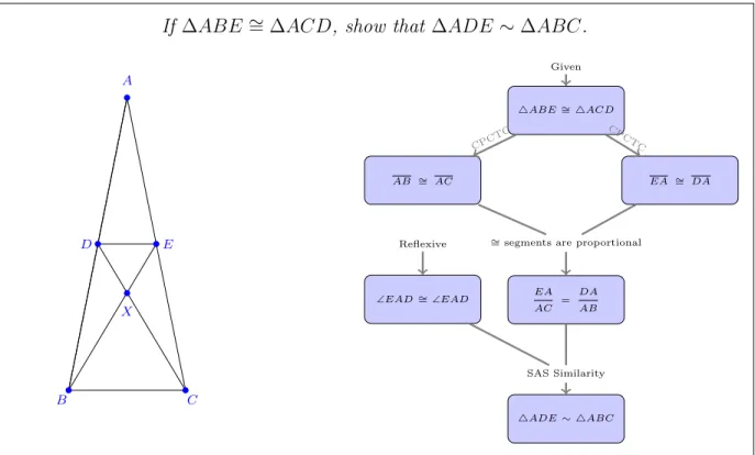
If ∆ABE ∼= ∆ACD, show that ∆ADE ∼∆ABC. 4ADE∼ 4ABC SAS Similarity ∠EAD∼=∠EAD EA AC = DA AB Reflexive AB ∼= AC EA ∼= DA
∼= segments are proportional 4ABE∼=4ACD Given CPCTC CPCTC B A C D E X
Figure 3.6: Example Problem and Minimal Solution Generated by GeoTutor
3.5 Problem Generation Interface
Before we present our problem synthesis algorithm, we provide a user’s view to in-teracting with our system: how the user may interact with our system to obtain a set of desired problems. The user provides a geometry figure drawn to scale and a set of axioms as inputs to the system, and can specify parameters to generate a desired set of problems with specific features.
3.5.1 Features of a Geometry Problem
A geometry problem P = (I, G) over a pair (Fig,Axm) has several features such as:
• The objects of the figure Fig and their properties I(Fig), E(Fig), e.g., the number of
points, triangles, etc.
• The size of the goal set |G|.
• The type of the goal, e.g., congruent triangles, equal segments, etc.
the assumptions to the goal in the proof), the width of a proof (maximal number of nodes in a level in the proof), the number of deduction steps (i.e., the number of hyperedges in the proof), and the number of axioms used. These features can be computed from the representation of proofs in the hypergraph.
• A subset of Axmthat occurs in every proof of the problem.
• Whether the problem is complete or not.
Our system allows defining arbitrary features as long as they are efficiently computable from the syntactic description of the problem or from the hypergraph representation.
3.5.2 Query Interface to Problem Generation
We propose an interface where the teacher can specify a relational query over the set of problem features and obtain a corresponding set of problems. We describe a semi-automated methodology to support this interface. Our methodology requires manual input
of (Fig,Axm) pairs. For each such pair, we generate the set of all interesting problems using
the problem generation technique described in §3.4. This set of problems, along with their
features, populate a relational database. We may then query the database using a standard
relational query (§3.6 gives examples of such queries with results in Table 3.2).
A student or teacher may define their own pair (Fig,Axm) using their own creativity
or directly from textbooks to generate fresh problems corresponding to that pair. In that respect, our methodology has a multiplicative effect: starting from the figure of a problem, our algorithms generate many more problems over the same figure.
3.6 Experimental Results
We first describe our benchmark set of problems and characteristics of the correspond-ing figures. Second, we evaluate our solution technique with respect to time required to construct the corresponding hypergraph and identify the solution path. Last, we corre-late structural characteristics of a solution with respect to the time taken to generate that solution.
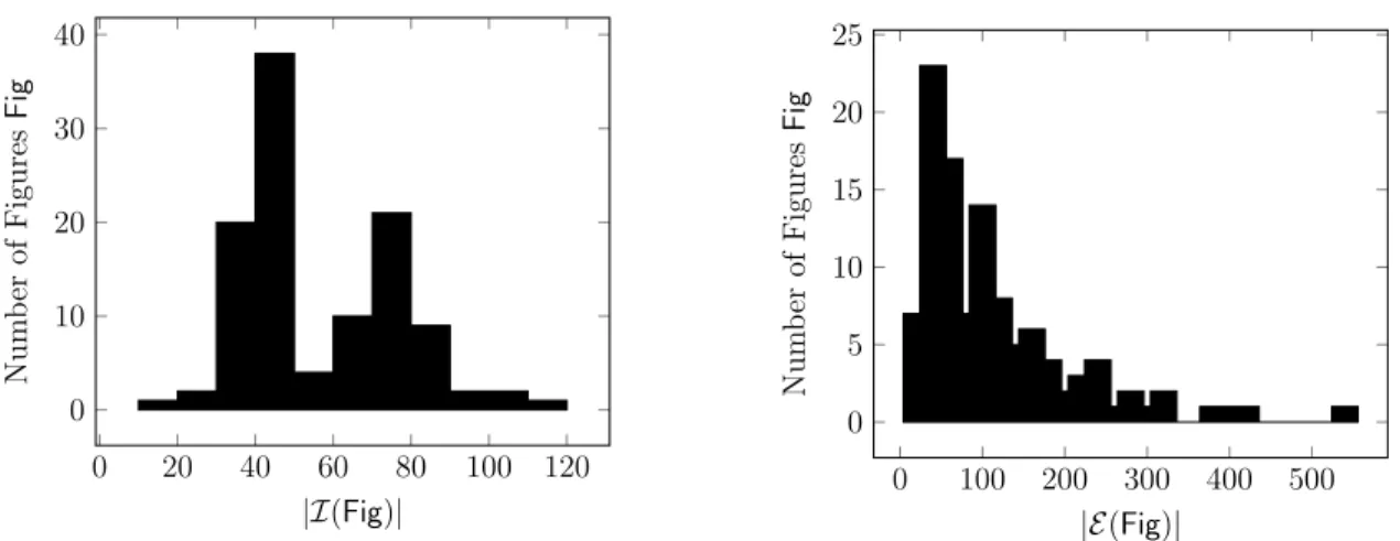
0 20 40 60 80 100 120 0 10 20 30 40 |I(Fig)| Num b er of Figures Fig 0 100 200 300 400 500 0 5 10 15 20 25 |E(Fig)| Num b er of Figures Fig
Figure 3.7: Histogram of|I(Fig)| and |E(Fig)| Per Figure F
3.6.1 Benchmark
We ran our problem generation algorithm on a set of 110 figures taken from standard mathematics textbooks in India [76, 75] as well as textbooks and workbooks popular in the United States [16, 56, 64, 51]. We used a uniform set of axioms for all of our experiments; this set included axioms related to parallel lines, congruent triangles, similar triangles, etc. The distribution of these 110 figures described by the number of the implicit facts per
figure, |I(Fig)|, is a bimodal distribution with modes around 40 and 75 and mean 46.5
as shown in Figure 3.7. The bimodal distribution indicates our attempt to balance our experiments with simple as well as more complex figures.
The distribution of these 110 figures described by the number of deduced facts per
figure, |E(Fig)|, is a positively-skewed distribution as shown in Figure 3.7 with mean 108,
median 82, and standard deviation 96.7. The skewed distribution indicates how few figures result in a large hypergraph making our problem generation algorithm often run efficiently in practice.
3.6.2 Evaluation of Algorithm GenProblem
We now present evaluation of our problem generation algorithm GenProblem with
1 2 3 4 5 6 0 10 20 30 40 50
|I|for Textbook Problem (I, G)
No. T ex tb o ok Problems ( I ,G )
Figure 3.8: Number of Assumptions |I| Per Textbook Problem (I, G)
those problems. We ran our experiments on a laptop with Intel Core i5-2520M CPU at 2.5GHz with 8 GB RAM on 64-bit Windows 7 operating system.
We modified GenProblem to only generate problems where |G| ≤ 2. This is because
our preliminary prototype encountered memory issues with |G| > 2 since the problem
generation procedure is exponential in |G|. For each (Fig,Axm) pair, we fixed I to be the
minimal set of assumptions that corresponded to the original textbook problem description
corresponding to the figure F. For the 110 figures we observed a mean of 2.3 assumptions
per figure with standard deviation 1.1; Figure 3.8 presents statistics on the size of this fixed minimal set per figure.
We found that complexity of the figure correlates with the length of time to process: more implicit facts in a figure results in more explicit facts and thus requires more time
to generate problems. Given a set of assumptions I over a pair (Fig,Axm), we determine
the Boolean classification whether I completely defines Fig. We may informally describe
a complete problem as a problem that is not open to interpretation. That is, complete problems are ideal for formal assessments. On the other hand, interesting problems are more malleable and therefore more applicable to homework or in-class investigations. Textbook problems are generally a mix of interesting and complete problems. We found for only 45
0 20 40 60 0 20 40 60 80 100 120
Figure Pairs (Fig,Axm)
No. Strictly In teresting Problems ( | G | = 1) (a) 0 10 20 30 40 0 20 40 60 80 100
Figure Pairs (Fig,Axm)
No. Strictly Complete Proble ms ( | G | = 1) (b)
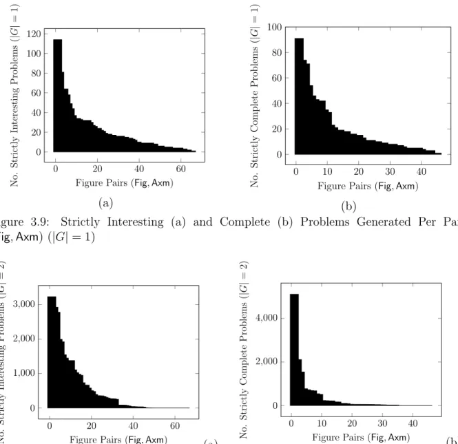
Figure 3.9: Strictly Interesting (a) and Complete (b) Problems Generated Per Pair
(Fig,Axm) (|G|= 1) 0 20 40 60 0 1,000 2,000 3,000
Figure Pairs (Fig,Axm)
No. Strictly In teresting Problems ( | G | = 2) (a) 0 10 20 30 40 0 2,000 4,000
Figure Pairs (Fig,Axm)
No. Strictly Complete Problem s ( | G | = 2) (b) Figure 3.10: Strictly Interesting (a) and Complete (b) Problems Generated Per Pair (Fig,Axm) (|G|= 2)
of 110 figures, the original textbook problem associated with it was complete. We expected a larger number of complete problems, but found that when drawing figures into our front-end slate, we were more likely to construct figures with unintfront-ended facts (e.g. points were likely to be midpoints, triangles likely to be isosceles or equilateral). This psychological factor lead to a greater number of original textbook problems being classified as interesting (but not complete).
Our methodology results in a large multiplicative effect: from a single pair (Fig,Axm) we are able to generate many problems. For the 65 of 110 original textbook figures that were classified as corresponding to interesting (but not complete) problems, we generated
a total of 1309 and an average of 20.1 strictly interesting problems (I, G) where |G| = 1;
the associated distribution is shown in Figure 3.9(a). For the remaining 45 of 110 original textbook figures, which were classified as corresponding to complete problems, we generated
a total of 877 and an average of 19.5 strictly complete problems (I, G) where |G|= 1 with
distribution in Figure 3.9(b). For |G|= 2, we generated 14760 strictly complete problems
and 31801 strictly interesting (but not complete) problems. When |G| = 2 we have an
empirical validation of the exponential growth in the number of generated problems. For
a fixed set of assumptions I, the definition of a strict problem dictates |I| ≥ |G| for
any G. Since many of our original textbook problems had |I| = 1, many figure pairs
(Fig,Axm) cannot generate problems with more than a single goal. The corresponding
distributions (shown in Figure 3.10) are heavily skewed with mean 489 and median 84 for strictly interesting (but not complete) problems as well as mean 328 and median 49 for strictly complete problems.
GenProblem took an average time of 4.7 seconds (with standard deviation of 10.5
seconds) per (Fig,Axm) pair to generate the above mentioned problems with|G| ≤2. For a
given (Fig,Axm) pair, the majority of the processing time is in construction of the saturated
hypergraph. Therefore, we expect a correlation between the number of explicit facts forFig
and the amount of time to process. As the worklist construction of H(Fig,Axm) requires
that we compare each newly deduced node against all existent nodes in H, we expect
hypergraph construction to be quadratic in the number of nodes in H; we have a strong
0 20 40 60 80 100 120 0
20 40 60
Figure Pairs (Fig,Axm)
No.
Problems
from
Query
Q
Figure 3.11: Problems Per Pair (Fig,Axm) for QueryQ={steps = 6 to 10,width = 4 to 8}
Let (Fig,Axm) be a pair where Fig is the
figure at right and Axmis our common set
of axioms.
A
D C
B M
The original problem from the textbook over (Fig,Axm) is (I, G), where
I ={Midpoint(M, BD), AM =M C,RightAngle(B, C, D)}
and
G={4BM C ∼=4DM A,RightAngle(A, D, C),4ADC ∼=4BCD,2BM =AC}.
The queryQgenerates several new problems of the form (I0, g0) over the pair (Fig,Axm),
where I0 =I and g0 takes on any of the following propositions.
• CD is an altitude of4ADC
• RightTriangle(A, D, C)
• AD⊥CD
• ADkBC
• ∠CDB and ∠M ADare
complemen-tary
Figure 3.12: Satisfying QueryQ overFig where Q={|G|= 1, s= 6−10, w = 4−8}
3.6.3 Effectiveness of Our Methodology
Once problems are generated from all pairs (Fig,Axm), we may obtain problems with