Automated methods for checking differential privacy

(1)

c

(2)

AUTOMATED METHODS FOR CHECKING DIFFERENTIAL PRIVACY

BY

VISHAL JAGANNATH RAVI

THESIS

Submitted in partial fulfillment of the requirements for the degree of Master of Science in Computer Science

in the Graduate College of the

University of Illinois at Urbana-Champaign, 2019

Urbana, Illinois Adviser:

(3)

ABSTRACT

Differential privacy is ade facto standard for statistical computations over databases that contain private data. The strength of differential privacy lies in a rigorous mathematical definition which guarantees individual privacy and yet allows for accurate statistical results. Thanks to its mathematical definition, differential privacy is also a natural target for formal analysis. A broad line of work uses logical methods for proving privacy. However, these methods are not complete, and only partially automated. A recent and complementary line of work uses statistical methods for finding privacy violations. However, the methods only provide statistical guarantees (but no proofs).

We propose the first decision procedure for checking differential privacy of a non-trivial class of probabilistic computations. Our procedure takes as input a programP parametrized by a privacy budget and either proves differential privacy for all possible values of , or generates a counterexample. In addition, our procedure applies both to-differential privacy and (, δ)-differential privacy. Technically, the decision procedure is based on a novel and judicious encoding of the semantics class of programs in our class into a decidable fragment of the first-order theory of the reals with exponentiation. We implement our procedure and use it for (dis)proving privacy bounds for many well known examples, including randomized response, histogram, report noisy max and sparse vector.

(4)

(5)

CHAPTER 5 DIPWHILE LANGUAGE . . . 19

CHAPTER 6 DECIDABILITY OF DIPWHILE PROGRAMS . . . 23

6.1 Parametrized DTMCs . . . 23

6.2 Semantics . . . 25

CHAPTER 7 DIPCTOOL . . . 38

7.1 Stages in Tool Development . . . 38

7.2 DiPC Usage . . . 41

CHAPTER 8 EXPERIMENTS . . . 46

8.1 Examples . . . 46

8.2 Experimental Results . . . 49

(6)

CHAPTER 1: INTRODUCTION

Differential privacy [1] is a gold standard for privacy of statistical computations. Differ-ential privacy ensures that running the algorithm on any two “adjacent” databases yields two “approximately” equal distributions, where two databases are adjacent if they differ in a single element, and two distributions are approximately equivalent if their distance is small w.r.t. some specific metric. Thus, differential privacy delivers a very strong form of individual privacy. Yet, and somewhat surprisingly, it is possible to develop differentially private algorithms for many tasks. Moreover, the algorithms are useful, in the sense that their results have reasonable accuracy. However, designing differentially private algorithms is difficult and the privacy analysis can be error-prone, as witnessed by the example of sparse vector. This difficulty has motivated the development of formal approaches for analyzing differentially private algorithms; see [2] for a survey and the related work section of this report.

Even though significant advances have been made in identifying proof principles to es-tablish differential privacy [3, 4, 5, 6, 7, 8, 9, 10] and techniques have been proposed to find differential privacy violations [11, 12], basic questions — Is checking differential privacy decidable? What are the limits of automated checking of differential privacy? What is the asymptotic complexity of checking? — have (shockingly) remained unanswered. The sole metric for evaluating proposed checking techniques has been experimental evaluation on ex-amples rather than a precise mathematical characterization of its limits. However, if past experience in automated formal verification of other application areas is any guide, then answering these foundational questions is essential for principled algorithmic development that is not only critical for theoretical advances but also for building practical tools that scale to large examples.

This report is a first attempt at addressing this serious lacuna in the current state of understanding in formal verification of differential privacy. Our first result establishes that checking differential privacy is indeed, computationally, a very difficult problem. We show that the problem of checking differential privacy is undecidable. Our proof of this result shows that the problem remains undecidable even if one considers programs with a single Boolean input, and a single Boolean output.

The main thrust of this report is, therefore, to identify a rich class of programs, that encompasses many known examples, for which checking differential privacy is decidable for all possible instances of the privacy parameter (throughout the report, we assume that the error parameter δ is defined as a function of ). Our undecidability proof highlights the

(7)

challenges in this enterprise — since it applies to really simple programs, can we even hope to find a practically relevant decidable fragment? We focus our attention on programs whose input and output spaces are finite. Note that such programs need not be finite state, as they could use auxiliary, variables, ranging over infinite domains, to carry out the computation. We introduce a class of programs, called DiPWhile, which are probabilistic while programs, for which the problem of checking differential privacy is decidable. We succeed in carefully balancing the twin (orthogonal) demands of decidability and expressivity, by judiciously delineating the use of real-valued and integer-valued variables. Our decidability proof for programs inDiPWhilehas the following salient features. The first step is an observation that the semantics ofDiPWhile-programs can be defined using parametrized, finite-state Markov chains 1_{. The fact that the semantics can be defined using only finitely-many states is a} surprising observation because our programs have integer and real-valued variables. Our key insight here is that a precise semantics forDiPWhile-programs can be given without tracking the explicit values of the real and integer-valued variables. Second, we observe that the transition probabilities of the Markov chain semantics are pseudo-rational functions of the privacy budget. These two observation together, allow us to reduce the problem of checking differential privacy ofDiPWhile-programs to the decidable fragment of the first order theory of reals with exponentials, identified by McCallum and Weispfenning [13].

Our decision procedure has two complementary uses. The first use of the procedure is a stand alone tool for checking - or (, δ())-differential privacy of mechanisms specified by DiPWhile-programs, for all values of . We have implemented our decision procedure in a tool that we call DiPC (Differential Privacy Checker). Given DiPWhile-program, our tool constructs a sentence in McCallum-Weispfenning fragment of the theory of reals with exponentials. It then calls MathematicaR

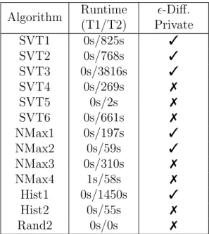
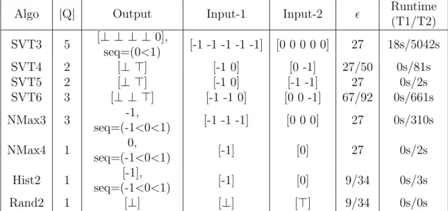
to check if the constructed sentence is true over the reals. Since our decision procedure is the first that can both prove differential privacy and detect its violation, we tried the tool on examples that known to be differentially private and those that are known to be not differentially private, including variants of Sparse Vector, Report Noisy Max, and Histograms. DiPC successfully checked differential privacy for the former class of examples and produced counterexamples for the later class. Our counter-examples are exact (rather than probabilistic) and are more compact than those delivered by prior tools.

A complementary use of the decision procedure is for validating counter examples for al-gorithms with infinite input or output sets. Our approach can be used to check-differential privacy of any mechanism for a given pair of adjacent input values and a given output value,

1_{A parametrized Markov chain is a Markov chain whose transition probabilities are a function of the}

(8)

for all values of >0, or for a given value of >0. It can also be used to find violations of programs with unbounded outputs. For such programs, it is possible to discretize the output domain into a finite domain, and to use the decision procedure to find privacy violations for the discretized algorithm (by post-processing, privacy violations for the discretized algo-rithms are also privacy violations for the original algorithm). Such usages complement the technique presented in [11] that proposes a method for generating counter examples. The approach of [11] is statistical in nature, and the examples generated by it are highly prob-able to be counter examples (with statistical guarantees), but may not be definite counter examples. Our approach can be used to check if the counter examples, generated by their tool, are real counter examples, for a given value of .

1.1 CONTRIBUTIONS

We summarize our key contributions.

• We prove the undecidability of the problem of checking differential privacy of very simple programs, including those that have a single Boolean input and output.

• We identify an expressive class of programs and give the first sound and complete method to verify differential privacy for a class of programs. That is, we present the first single,fully automatic method that can prove both prove differential privacy and detect its violation by generating counterexamples; hitherto all previous approaches can either only prove differential privacy or only prove its violation, but not do both. • We implement the decision procedure and evaluate our approach on private and

non-private examples of the literature.

1.2 TOOL AND EXPERIMENTS

The tool and experiments are available at the anonymous url [14].

1.3 RELATED WORK

The main thread of work has focused on formal systems for proving that an algorithm is differentially private. Such systems are helpful because they rule out the possibility of mistakes in privacy analyses. Reed and Pierce [3] propose the first programming language technique for proving differential privacy, in the form of a linear type system. Gaboardi et

(9)

al [4] later enrich their approach with linear dependent types, in order to support recursion and a broader set of differentially private constructions. Azevedo de Amorim et al [9] propose another extension to accommodate (, δ)-differential privacy. However, it is not possible to verify some of the most advanced examples, such as sparse vector or vertex cover, using these type systems. Moreover, type-checking and type-inference for linear (dependent) types is challenging. Barthe et al [5, 6, 7] develop several program logics for reasoning about differential privacy. These logics construct approximate probabilistic couplings between two program executions on adjacent inputs. These couplings are parametrized by a binary relation on program outputs; when specialized to the equality relations, these approximate probabilistic couplings coincide with the notion of approximate equality used in differential privacy. These logics have been used successfully to analyze many classic examples from the literature, including the sparse vector technique. However, these logics are limited: they cannot disprove privacy; extensions may be required for specific examples; building proofs is challenging. The last issue has been addressed by Zhang and Kifer [8] and by Albarghouthi and Hsu [10]. These works propose automated methods for proving automatically differential privacy. Zhang and Kifer introduce randomness alignments as an alternative to couplings, and build a dependent type system that tracks randomness alignments. Automation is then achieved by type inference. Albarghouthi and Hsu propose coupling strategies, which rely on a fine-grained notion of variable approximate coupling which draws inspiration both from approximate couplings and randomness alignment. They synthesize coupling strategies by considering an extension of Horn clauses with probabilistic coupling constraints, and developing algorithms to solve such constraints. However, these methods are limited to vanilla-differential privacy and do not accommodate bounds that are obtained by advanced composition (sinceδ 6= 0). Recently, Liu, Wang, and Zhang [15] develop a probabilistic model checking approach for verifying differential properties. Their approach is based on modelling differential private programs as Markov chains. Their encoding is more direct than ours (i.e. it does not attempt to build a finite-state Markov chain) and they do not provide a decision procedure. Chistikov and Murawski and Purser [16] propose an elegant method based on skewed Kantorovich distance for checking differential privacy of Markov chains. However, their approach is rather theoretical and not implemented.

A dual problem is to automatically find violations of differential privacy. This would help privacy practitioners discover potential problems in their algorithms as early as possible. Two recent and concurrent works by Ding et al [11] and Bischel et al [12] develop automated methods for finding privacy violations. Ding et al propose an approach which combines purely statistical methods based on hypothesis testing and symbolic execution. Bischel et al develop an approach based on a combination of optimization methods and language-specific

(10)

techniques for computing differentiable approximations of privacy estimations. Both meth-ods are fully automated. However, their guarantees are statistical (no proofs). Moreover, both methods can only be used for concrete numerical values of the privacy budget . As previously explained, our work is complementary to these approaches, in the sense that our decision procedure can be used to verify their proposed counter-examples (for algorithms that fall in the class of programs handled by the procedure).

To our best knowledge, no prior work is able to both prove differential privacy and detect its violations for a non-trivial class of programs.

Our work is also loosely connected to prior attempts to relate differential privacy and information flow. In particular, Barthe and K¨opf [17] study information-theoretic bounds for differentially private channels and provide a decision procedure for rational bounds. Their decision procedure is based on a reduction to the theory of real closed fields (without exponential). However, there approach considers channels and is not directly applicable to a language-based setting.

(11)

CHAPTER 2: PRIMER ON DIFFERENTIAL PRIVACY

Differential privacy [1] is a rigorous definition and framework for private statistical data mining. In this model, a trusted curator with access to the database returns answers to queries made by possibly dishonest data analysts that do not have access to the database. The curator’s task is to return probabilistically noised answers, so that data analysts cannot distinguish between two databases which are adjacent, i.e. only differ in the value of a single individual. There are two common definitions: two databases are adjacent if they are exactly the same except for the presence or absence of one record, or exactly the same except for the difference in one record. We abstract away from any particular definition of adjacency.

Henceforth, we denote the set of real numbers, rational numbers, natural numbers and integers by _R,_Q,_N, and _Z respectively. The Euler constant shall be denoted by e. We assume given a set U of inputs, and a setV of outputs. A randomized function P fromU to V is a function that takes an input inU and returns a distribution overV. For a measurable set S ⊆ V, the probability that the output of P on u is in the set S shall be denoted by Prob(P(u)∈S). In the case the output set is discrete, we use Prob(P(u) = v) as shorthand for Prob(P(u) = {v}).

We are now ready to define differential privacy. We assume that U is equipped with a binary symmetric relation Φ ⊆ U × U, which we shall call the adjacency relation. We say that u1, u2 ∈ U are adjacent if (u1, u2)∈Φ.

Definition 2.1. Let ≥ 0 and 0 ≤ δ ≤ 1. Let Φ ⊆ U × U be an adjacency relation. Let P be a randomized function with inputs from U and outputs in V. We say thatP is (, δ)-differentially private with respect to Φ if for all measurable subsets S ⊆ V and u, u0 ∈ U such that (u, u0)∈Φ,

Prob(P(u)∈S)≤eProb(P(u0)∈S) +δ

As usual, we say that P is -differentially private iff it is (,0)-differentially private. If the output domain is discrete, it is equivalent to require that for all v ∈ V and u, u0 ∈ U such that (u, u0)∈Φ,

Prob(P(u) = v)≤eProb(P(u0) = v)

Differential privacy is preserved by post-processing. Formally, ifP is an (, δ)-differentially private computation from U toV, and h:V → W is a deterministic function, thenh◦P is an (, δ)-differentially private computation from U toW. In the remainder, we shall exploit post-processing to connect differential privacy of randomized computations with infinite

(12)

output spaces to differential privacy of their discretizations.

Laplace Mechanism

The Laplace mechanism [1] achieves differential privacy for numerical computations by adding random noise to outputs. Given >0 and mean µ, let Lap(, µ) be the continuous distribution whose probability density function (p.d.f.) is given by

f,µ(x) =

2 e

−|x−µ|

.

Lap(, µ) is said to be theLaplacian distributionwith meanµand scale parameter1.Consider a real-valued function q:U → _R. Assume that q is k-sensitive w.r.t. an adjacency relation Φ on U, i.e. for every pair of adjacent values u1 and u2, |q(u1)−q(u2)| ≤ k. Then the computation that mapsu to Lap(_k, q(u)) is -differentially private.

It is sometimes convenient to consider the discrete version of the Laplace distribution. Given >0 and meanµ, letDLap(, µ) be the discrete distribution on_Z, the set of integers, whose probability mass function (p.m.f.) is given by

f,µ(i) =

1−e−

1 +e− e

−|i−µ|

.

DLap(, µ) is said to be thediscrete Laplacian distribution with meanµand scale parameter 1

. The discrete Laplace mechanism achieves the same privacy guarantees as the continuous

Laplace mechanism.

Exponential mechanism

The Exponential mechanism [18] is used for making non-numerical computations private. The mechanism takes as input a value u from some input domain and a scoring function F :U × V →_Rand outputs a discrete distribution overV. Formally, given >0 andu∈ U, the discrete distributionExp(, F, t) on V is given by the probability mass function:

h,F,t(v) =

eF(t,v)

P

v∈VeF(t,v)

.

Suppose that the scoring function is k-sensitive w.r.t. some adjacency relation Φ on U, i.e., for all for each pair of adjacent values u1 and u2 and v ∈ V, |F(u1, r)−F(u2, r)| ≤k. Then the exponential mechanism is (2k,0)-differentially private w.r.t. Φ.

(13)

CHAPTER 3: MOTIVATING EXAMPLES

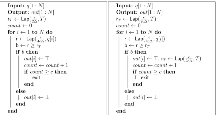
Before presenting the mathematical details of our results, let us informally present our method by showing how it would work on some illustrative examples. Consider the Sparse Vector Technique (SVT) [19, 20]. The Sparse Vector Technique was designed to answer multiple ∆-sensitive numerical queries in a differentially private fashion. The relevant infor-mation we want from queries is, which amongst them are above a threshold T. If we apply a differentially private mechanism to answer each one of them separately then the privacy budget explodes (answering k such queries in an -differentially private manner would only be k-differentially private). The SVT as given in Algorithm 3.1 is designed to identify the first c queries that are above the thresholdT in an -differentially private fashion.

Input: q[1 :N] Output: out[1 :N] rT ←Lap(_2∆ , T) count←0 for i←1 to N do r←Lap(₄_c_∆, q[i]) b←r≥rT if b then out[i]← > count←count+ 1 if count≥c then exit end else out[i]← ⊥ end end Algorithm 3.1:SVT algorithm (SVT1)

In the program, the integer N represents the total number of queries and the array q of length N represents the answers to queries. The array out represents the output array, ⊥ represents False and>represents True. We assume that initially the constant⊥is stored at each position inout. In the SVT technique, the true answers account for most of the privacy cost and we can only answer c of them until we run out of the privacy budget [19, 8]. On the other hand, there is no restriction to the false answers that can be given.

(14)

q[k] represents the answer to thekth query on the original database. The adjacency relation Φ on inputs is defined as follows: q1 and q2 are adjacent if and only if |q1[i]−q2[i]| ≤ 1 for each 1≤i≤N.

Let us consider an instance of the SVT algorithm when T = 0, N = 2, ∆ = 1 and c = 1. Let us assume that all array elements in q come from the domain {0,1}. In this case, we have four possible inputs [0,0],[0,1],[1,1], and [1,0], and three possible outputs [⊥,⊥],[>,⊥], and [⊥,>]. Our approach is to compute, for each input x and output y, the probability of returning y when the input is x. Note that this probability depends on the parameter , and so what we are looking for is a symbolic representation of this function. For example, the probability of outputting [⊥,>] on input [0,1] is

r1 = 24e34 −1 + 8e 4 + 21e 2 48e34 .

Similarly, when the input is [1,1] and the output is [⊥,>], the probability is given by r2 =

−22 + 32e4 −3

48e2

.

Our goal is to compute expressions like r1 and r2 automatically from the program, input, and output. Having computed such expressions, checking -differential privacy requires one to determine if

for all >0.(r1 ≤er2) and for all >0.(r2 ≤er1).

Notice that the above conditions can be encoded as a first order sentence with exponen-tials, and checking if -differential privacy holds, reduces to determining if such a first order sentence is true for reals, with the standard interpretation of multiplication, addition, and exponentiation. Whether there is a decision procedure that can determine the truth of first order sentences involving exponentials over the reals, is a long standing open problem. How-ever, certain decidable fragments of such an extended first order theory have been identified. Our main result shows that for many examples, checking differential privacy can be reduced to a decidable fragment identified by McCallum and Weispfenning [13].

Notice that if one can compute expressions for the probability producing certain outputs on a given input, we could use the above ideas to also check (, δ)-differential privacy, instead of just -differential privacy. The only change would be to account for δ in our constraints, and to consider all possible subsets of outputs, instead of just individual output values. Thus, the methods proposed here go beyond the scope of most automated approaches, which are

(15)

restricted to vanilla -differential privacy.

3.1 FINITE DISCRETIZATION OF INFINITE OUTPUT SPACES

As outlined in the introduction, our decision procedure checks differential privacy of pro-grams whose output space is finite. In many examples, the program outputs are reals or unbounded integers (and combinations thereof). Nevertheless, we argue that our decision procedure can still be used in the verification of differential privacy. Our approach in such cases is to discretize the output space into finitely many intervals.

We illustrate this for the special case when a program P outputs the value of one real random variable, sayr. Now, suppose that we modifyP to output a finite discretized version of r as follows. Let seq=a0 < a1 < . . . an be a sequence of rationals and let

Discseq(x) =                      a0 x≤a0 a1 a0 < x≤a1 .. . an−1 an−2 < x≤an−1 an otherwise .

Consider the program PDisc,seq that instead of outputting r, outputs Discseq(r). It is easy to see that if P is differentially private then so must be PDisc,seq. Therefore, if PDisc,seq is not differentially private then we can conclude that PDisc,seq is not differentially private. Our decision procedure is both sound and complete for a class of programs we identify. Therefore, we can use our method to find counterexamples; counterexamples for us is a pair of adjacent inputs and a value of that violates the differential privacy inequation. Thus, if our decision procedure finds a counterexample for PDisc,seq, then it also has proved that P is not differentially private. Our method can, therefore, be used as an under-approximation technique for checking differential privacy of P. In fact, it is complete under-approximation method in the sense that P is differentially private iff for each possible seq, PDisc,seq is differentially private.

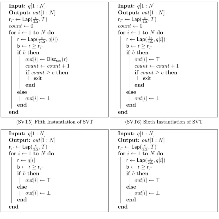
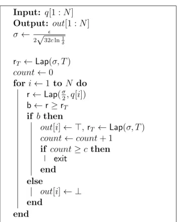
Let us illustrate the discretization approach to detecting privacy violations through an example. One variant of SVT algorithm is one in which the algorithm outputs noisy queries that are above the noisy threshold (and not just which queries are above the threshold). This algorithm outputs real values and is known to violate differential privacy [20]. As discussed above, while we cannot model this algorithm directly in our framework, we can model its

(16)

Input: q[1 :N] Output: out[1 :N] rT ←Lap(_2∆ , T) count←0 for i←1 to N do r←Lap(₄_c_∆, q[i]) b←r≥rT if b then out[i]←Discseq(r) count←count+ 1 if count≥c then exit end else out[i]← ⊥ end end

Algorithm 3.2: Discretized SVT algorithm that outputs noisy queries above noisy threshold (SVT3)

discretized version. The discretized version is given in Algorithm 3.2.

Consider the instance of this discretized algorithm with N = 5, c = 1,∆ = 1, T = 0 and let seq consist of a single rational number 0. Consider input i1 = [0,0,0,0,0] and output o = [⊥,⊥,⊥,⊥,0]. The probability of producing o on input i1 is p1 = ₁₃₄₄1 . On the other hand, the probability that o is produced on input i2 = [1,1,1,1,0] is p2 = e

−5

4

1344. Now -differential privacy would require that

diff =p1−ep2 = 1 1344 −

e−4

1344

be ≤ 0. However, this is not true, for example, when = 27. This counterexample was found automatically by our tool DiPC.

We conclude this chapter by pointing out that the discretization technique also allows us to complement existing statistical techniques for finding counterexamples to differential privacy. Such statistical techniques [11] assume a fixed and typically produce a candidate counterexample which is pair of adjacent inputs in1, in2 and an output set S (usually an interval Iout = (a, b)). These techniques do not provide a method for checking whether this is a real counterexample or just a statistical anomaly. Our methods can then serve to check that this candidate counterexample is really a counterexample by taking seq=a < b.

(17)

CHAPTER 4: CHECKING DIFFERENTIAL PRIVACY

We consider the problem of verifying the differential privacy of randomized algorithms. Typically, such algorithms are modeled as a programP parametrized by a value. Having a

paramterized program P captures the fact that program’s behavior depends on the privacy

budget , with the intention of guaranteeing that P is (f(), g())-differentially private,

where f and g are some functions of . The parameter is assumed to belong to some (potentially unbounded) interval I ⊆_R>0 _{with rational endpoints; usually, we take} _{to just} belong to the interval (0,∞). The programP will be assumed to terminate with probability

1 for every value of (in the appropriate interval).

We will assume that our programs take inputs from a set U and produce outputs over a setV. In this report, we will assume that bothU andV are finite sets that can be effectively enumerated. Despite our restriction to finite input and output sets, as we will see in the next section (Section 4.1), the computational problem checking differential privacy is challenging. At the same time, the decidable subclasses we identify (Sections 4.2 and 5), are rich enough to model most known differential privacy mechanisms even though they have finite input and output sets. Extending our decidability results to subclasses of programs that have infinite input and output sets, is a non-trivial open problem at this time.

The computational problems we consider in this report are as follows. Since our programs take inputs from a finite setU, we assume that the adjacency relation Φ ⊆ U × U is given to us as an explicit list of pairs. In general, when discussing (, δ)-differential privacy of some mechanism, the additive parameterδneeds to be a function of. To define the computational problem of checking differential privacy, the functionδ :_R>0 _→_[0,_{1] must be given as input.} We, therefore, assume that this functionδhas some finite representation; ifδ is the constant δ0 then we represent δ simply by the number δ0. There are two computational problems we consider in this report.

Fixed Parameter Differential Privacy Given a problem P over inputs U and outputs

V, adjacency relation Φ ⊆ U × U, and rational numbers 0, δ0, t ∈ Q>0, determine if

P0 is (t0, δ0)-differentially private with respect to Φ.

Differential Privacy Given a program P over inputs U and outputsV, interval I ⊆R>0,

δ : _R>0 _→ _[0,_{1], an adjacency relation Φ} _{⊆ U × U}_{, and a rational number} _t _∈

Q,

determine if P is (t, δ())-differentially private with respect to Φ for every ∈I.

Observe that the Fixed Parameter Differential Privacy problem can be trivially reduced to the Differential Privacy problem. Thus, an algorithm for checking Differential Privacy can

(18)

be used to solve Fixed Parameter Differential Privacy. Unfortunately, the Fixed Parameter Differential Privacy problem is extremely challenging — we will show that it is undecidable, and therefore, so is the Differential Privacy problem. We will conclude this chapter by identifying semantic conditions under which the Differential Privacy problem (and therefore the Fixed Parameter Differential Privacy problem) is decidable.

4.1 UNDECIDABILITY OF DIFFERENTIAL PRIVACY

The main result in this section is that the Fixed Parameter Differential Privacy problem is undecidable. Consider simple while programs that have variables storing Booleans and integers. Program statements are either assignments, random assignments that sample from discrete Laplacians, conditional statements, and loops. Let us denote this class of programs by Simple; in the interests of space, we skip the formal definition of such programs, relying instead on the reader’s informal understanding. Inputs to such programs (i.e. set U) are valuations to input program variables. We have the following undecidability result.

Theorem 4.1. The Fixed Parameter Differential Privacy problem and the Differential Pri-vacy problem for programs P in Simpleis undecidable.

Proof. We shall prove this by reducing the non-halting problem for deterministic 2-counter Minsky machines (which is known to be undecidable) to the Fixed Parameter Differential Privacy problem.

Recall that a 2-counter Minsky Machine is tuple M= (Q, qs, qf,∆1inc,∆2inc,∆1jzdec,∆

2

jzdec)

where

• Q is a finite set of control states. • qs∈Q is the initial state.

• qf ∈Q is the final state.

• ∆i

inc⊆Q×Qis the increment of counter ifor i= 1,2.

• ∆i_jzdec⊆Q×Q×Q is the conditional jump of counter i fori= 1,2.

Mis said to be deterministic if from each state q, there is at most one transition out of q. The semantics ofMis defined in terms of a transition system (Conf,(qs,0,0),→) where

Conf =Q×_N×_N is the set of configurations, (qs,0,0) is the initial configuration and →

(19)

(q, i, j)→(q0, i+ 1, j) if (q, q0)∈∆1 inc, (q, i, j)→(q0, i, j+ 1) if (q, q0)∈∆2 inc, (q, i, j)→(q0, i, j) if i= 0 and (q, q0, q00)∈∆1 jzdec, (q, i, j)→(q00, i−1, j) if i6= 0 and (q, q0_{, q}00₎_∈_∆1 jzdec, (q, i, j)→(q0, i, j) if j = 0 and (q, q0, q00)∈∆2 jzdec,and (q, i, j)→(q00, i, j−1) if j 6= 0 and (q, q0_{, q}00₎_∈_∆2 jzdec.

We show that given a 2-counter Minsky Machine M, there is a program PM ∈ Simple such that for each >0,

(a) PM has only one Boolean input bin and one Boolean outputbout. (b) PM terminates with probability 1.

(c) PMis (,0)-differentially private w.r.t adjacency relation Φ ={(true,false),(false,true)} if and only if Mdoes not halt.

A sequence of configurationss0, s1, . . . sk is said to be a computation ofMif s0 = (qs,0,0)

and si → si+1 for i = 0,1, . . . k − 1. A computation s0, s1, . . . sk is said to be a halting

computation ofM if sk = (qf, i, j) for some i, j ∈N.

Given a 2-counter MachineM, PM

is constructed as follows. First we observe that without

loss of generality we can assume that the set of states Q of M can are integers 1,2, . . . , m where m is the number of states in Q. Thus, a configuration of M can be encoded as three integers state,cntr1,cntr2. The transition relations ∆1_inc,∆2_inc,∆1_jzdec and ∆2_jzdec can be encoded using 3 additional counters,n state,n cntr1,n cntr2,which model the next state and the the next counter values. For example, the transition (q, q0, q00)∈∆1

jzdec can be encoded

using conditional statements as follows:

if (cntr1 = 0) and (state=q) then n state=q0; end if (cntr1 >0) and (state=q) then n state=q00;n cntr1 =n cntr1−1; end

Lets1, s2, . . . , snbe the statements encoding the transition relation. Consider the program

PM given in Figure 4.1. The programPM initially samplesk from a discrete Laplacian. If the sampled value is <0 then it outputs false. Otherwise, it simulates M upto k. At the

(20)

Input: bin Output: bout bout ←false k ←DLap(,0) if k >0 then state←qs cntr1 ←0 cntr2 ←0 for steps←1 to k do s1 .. . sn state←n state cntr1 ←n cntr1 cntr2 ←n cntr2 end

if (state=qf) and (bin=true) then bout ←true

end end

Algorithm 4.1:Program PM simulating 2-counter machine M

end of the simulation, if the halting state is reached and the input is true then it outputs true. Otherwise, it outputs false.

Clearly, PM satisfies properties (a) and (b) above. That the program PM has property (c) above follows from the following observations:

1. If M does not halt then PM outputs false with probability 1.

2. If Mhalts thenPM outputstrue with non-zero probability on inputtrue and outputs true with zero probability on input false.

This shows that Fixed Parameter Differential Privacy is undecidable. Undecidability of Fixed Parameter Differential Privacy is obtained by taking 0 to be any constant rational

number, say 1₂. q.e.d

This theorem shows that Differential Privacy is undecidable. Undecidability of Fixed Parameter Differential Privacy is obtained by taking 0 to be any constant rational, say 1₂.

(21)

4.2 A TRACTABLE SEMANTIC CLASS OF PROGRAMS

Since the problem of checking differential privacy is undecidable (Theorem 4.1) it is nec-essary to restrict the class of programs to get a decision procedure. The program PM constructed in the proof of Theorem 4.1 is an extremely simple program. This demonstrates how challenging the task of identifying a tractable, yet useful, subset of programs is. In this section, we identify a simple semantic restriction under which the Fixed Parameter Differential Privacy and Differential Privacy problems are decidable. In Chapter 5, we will use the results of this section to prove that the problem of checking differential privacy is decidable for programs written in ourDiPWhilelanguage. Our goal in identifying a semantic restriction is to reduce the problem of checking differential privacy to checking the truth of a first order formula involving exponentials about the reals. Decidability of the theory of reals with exponentials is a long standing open problem, related to Schanuel’s conjecture. Some fragments of this theory are known to be decidable. In particular, McCallum and Weispfenning [13] have identified a decidable fragment of the first order theory of reals with exponentials, that we will exploit. Therefore, before defining our semantic restriction, we introduce this decidable first order theory.

We will consider first order formulas over a restricted signature and vocabulary. We will denote this collection of formulas as the language Lexp. Formulas in Lexp are built using variables {} ∪ {xi|i ∈ N}, constant symbols 0,1, unary relation symbol e(·) applied only

to the variable , binary function symbols +,−,×, and binary relation symbols =, <. The terms in the language are integral polynomials with rational coefficients over the variables {} ∪ {xi |i ∈ N} ∪ {e}. Atomic formulas in the language are of the form t = 0 or t < 0

or 0 < t, where t is a term. Quantifier free formulas are Boolean combinations of atomic formulas. Sentences in Lexp are formulas of the form

QQ1x1· · ·Qnxnψ(, x1, . . . xn)

where ψ is a quantifier free formula, and Q, Qis are quantifiers. In other words, sentences

are formulas in prenex form, where all variables are quantified, and the outermost quantifier is for the special variable .

We will be interested in an extension of the first order theory of reals. That is, the theory Thexpis the collection of all sentences inLexpthat hold in the structurehR,0,1, e(·),+,−,×,= , <i, where the interpretation for 0,1,+,−,× is the standard one on reals, and e is Euler’s constant. The crucial property about this theory is that it is decidable.

(22)

Our tractable semantic restriction on programs relies on certain special functions of type I →_R, namely those that are definable inThexp. A functionf :I →Ris said to bedefinable

inThexp, if there is a formula ϕf(, x) in Lexp with two free variables ( and x) such that f(a) =b iff h_R,0,1, e(·),+,−,×,=, <i |=ϕf(, x)[7→a, x7→b]

A sufficient condition to ensure the decidability of checking differential privacy is to con-sider programs with the property that for each input, the probability distribution on the outputs is definable inThexp. This identifies the semantic restriction we will consider in this section.

Definition 4.3. A parametrized programPwith inputsU and outputsV is said to identify a

definable distributiononV if for eachin∈ U andout∈ V the function7→Prob(P(in) = out)

is definable in Thexp.

A parametrized program P with inputs U and outputs V is said to effectively identify a

definable distribution onV if there is an algorithmAsuch that for each in∈ U andout ∈ V, A outputs a formula ϕin,out(, x) in Lexp that defines the function 7→Prob(P(in) = out).

The main result of this section is that checking differential privacy for programs that effectively identify a definable distribution is decidable.

Theorem 4.4. The Fixed Parameter Differential Privacy and Differential Privacy problems are decidable for programsP that effectively identify a definable distribution and definable

functions δ (in the case of the Differential Privacy problem).

Proof Sketch. We sketch the decidability proof for the Differential Privacy problem; the proof also contains all the necessary ideas to establish the decidability of Fixed Parameter Differential Privacy problem. Let P be a program that effectively identifies a definable

distribution with adjacency relation Φ. Let us assume that the formula ϕin,out(, xin,out) of Lexp defines the function 7→ Prob(P(in) = out). Let ϕδ(, xδ) be the formula defining the

function δ. Let t= p_q where p, q are natural numbers. We show the proof when I is (0,∞). It is easy to modify the proof for any interval I with rational end-points.

Consider the sentence

ψ =∀.∀z.[∀xin,out]in∈U,out∈V.∀xδ.

(( >0)∧(ep=zq)∧(z >0) ∧ϕδ(, xδ)

V

in∈U,out∈V ϕin,out(, xin,out)) →(V

(in1,in2)∈Φ,O⊆V P

out∈Oxin1,out <

zP

(23)

It is easy to seeP is differentially private for alliffψis true over the reals. In the syntax of

Lexp, we cannot takeqth roots ofe; therefore, we introduce the variablez, which enables us to write the constraints using onlyea_{, where}_a_∈

N. Notice thatψ belongs toLexpif we convert it to prenex form. Decidability therefore follows from the decidability of Thexp. q.e.d IfPis not differentially private, then the sentenceψdoes not hold. The decision procedure

for Thexp will in this case return an that witnesses the non-privacy of P. This could be

used to construct counterexamples.

Definition 4.5. A counterexample forP, with respect to an adjacency relation Φ, a function

δ :_R>0 _→_[0,_{1] and a value} _t _∈

Q, is a quadruple (u, u0, S, 0) such that (u, u0) ∈Φ, S ⊆ V and 0 >0 and

Prob(P0(u)∈S)> et0Prob(P(u0)∈S) +δ(0) When δ is the constant function 0, then S is {v} for some v ∈ V.

(24)

CHAPTER 5: DIPWHILE LANGUAGE

We now introduce the language DiPWhile for which differential privacy can be checked effectively (Chapter 6). Informally, DiPWhile is a syntactically restricted class of proba-bilistic while programs, having variables that take values from either Booleans, a finite set DOM (to model variables taking finite values), integers, or reals. Probabilistic steps in the language correspond to sampling using either the Laplace, discrete Laplace, or exponential mechanisms. We also allow probabilistic steps where values inDOMare sampled from a user defined distribution. The key restrictions we impose are as follows. First, we assume that real and integer variables are never assigned inside the scope of a while loop. This ensures that any real (or integer) variable is given a value only abounded number of times. Second, loop and branch conditionals never depend on comparing values stored in real variables with values stored in integer variables. These restrictions are crucially exploited in our decid-ability proof. The informal reasons behind them can be best understood in the context of defining the semantics for DiPWhile programs and so are postponed to Section 6.2.

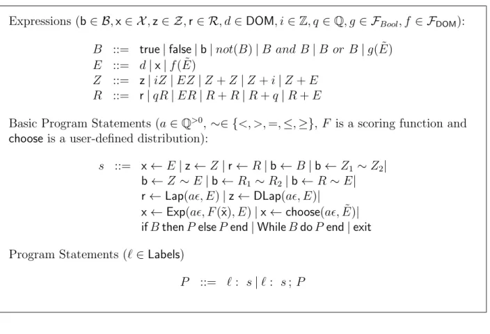
The formal syntax of DiPWhile, that makes precise the restrictions outlined above, is shown in Figure 5.1. We have four types for variables: Bool = {true,false}; finite domain DOM that we assume (without loss of generality) to be {−Nmax, . . .0,1, . . . Nmax}, a finite subset of integers1; reals_R; and integers_Z. The set of Boolean/DOM/integer/real program variables are respectively denoted by B/X/Z/R. The set of Boolean/DOM/integer/real expressions is given by the non-terminalB/E/Z/R in Figure 5.1. We now explain the rules for such expressions. Boolean expressions (B) can be built using Boolean variables and constants, standard Boolean operations, and by applying functions from FBool. FBool is

assumed to be a collection of computable functions returning a Bool. DOM expressions (E) are similarly built from DOM variables, values in DOM, and applying functions from set of computable functions FDOM. Next, integer expressions (Z) are built using multiplication and addition with integer constants andDOM expressions, and additions with other integer expressions. Finally, real expressions (R) are built using multiplication and addition with rational constants and DOM expressions, and additions with other real-valued expressions.

A program in our language is a triple consisting of a set of (private) input variables, a set of (public) output variables, and a finite sequence of labeled statements (non-terminalP in Fig-ure 5.1). The private input variables and public output variables take values from the domain DOM. Thus, the set of possibles inputs/outputs (U/V), is identified with the set of valuations for input/output variables; a valuation over a set of variablesX0 ={x1,x2, . . . ,xm} ⊆ X is a

(25)

E ::= d|x|f( ˜E)

Z ::= z|iZ|EZ|Z+Z|Z +i|Z +E R ::= r|qR|ER|R+R|R+q|R+E

Basic Program Statements (a∈_Q>0_, _{∼∈ {<, >,}_=,_≤,_≥}, _F _{is a scoring function and} choose is a user-defined distribution):

s ::= x←E|z←Z|r←R|b←B|b←Z1 ∼Z2| b←Z ∼E|b←R1 ∼R2|b←R ∼E| r←Lap(a, E)|z←DLap(a, E)|

x←Exp(a, F(˜x), E)|x←choose(a,E˜)| ifBthenP elsePend|WhileBdoPend|exit Program Statements (`∈Labels)

P ::= ` : s|`: s; P

Figure 5.1: BNF grammar for DiPWhile. DOM is a finite discrete domain. FBool, (FDOM resp) are set of functions that output Boolean values (DOM respectively). B,X,Z,R are the sets of Boolean variables, DOM variables, integer random variables and real random variables. Labelsis a set of program labels. For a syntactic class S, ˜S denotes a sequence of elements from S.

function from X0 to DOM. Note that if we represent the set X0 as a sequence x1,x2, . . . ,xm

then we can represent a valuation val over x as a sequence val(x1), val(x2), . . . , val(xm) of

elements from DOM.

We assume every statement in our program is uniquely labeled from a set of calledLabels. Statements (non-terminal s) can either be assignments, conditionals, while loops, or exit. Statements other than assignments are self-explanatory. The syntax of assignments is de-signed to follow a strict discipline. Real and integer variables can either be asde-signed the value of real/integer expression or samples drawn using the Laplace or discrete Laplace mechanism. DOM variables are either assigned values of DOM expressions or values drawn either using an exponential mechanism (Exp(a, F(˜x), E)) or a user defined distribution (choose(a,E)).˜ For the exponential mechanism, we require that the scoring function F be computable and return a rational value. Both these restrictions are unlikely to be severe in practice, but are needed to ensure decidability. In the case of the user defined distribution, we demand that

(26)

the probability with which a value in DOM is chosen (as function of the privacy budget ), be definable in Thexp. Again this is needed to ensure decidability. Finally, we consider as-signments to Boolean variables. The interesting cases are those where the Boolean variable stores the result of the comparison of two expressions. As mentioned at the beginning of this section, we do not allow that comparison between real and integer expressions; this is reflected in the syntax. In addition to the above syntactic restrictions, DiPWhile programs will adhere to the following principles.

Bounded Assignments We do not allow assignments to real and integer variables within the scope of a while loop. This ensures that assignments to such variables happen only abounded number of times during an execution. Therefore, without loss of generality, we will assume that real and integer variables are assignedat most once.

Define Before Use We will assume that in any execution, if a variable appears on the right side of an assignment statement, then it should have been assigned a value before. The DiPWhile language is surprisingly expressive — many known randomized algorithms for differential privacy can be encoded. We give examples of such encodings in DiPWhile. We omit labels of program statements unless they are needed.

Example 5.1. Figure 5.1 shows howSV T can be encoded in our language withT = 0,∆ = 1, N = 2, c = 1. In the example we are modeling ⊥ by 0 and > by 1. Please observe that although we do not have For loops in our program, we can nevertheless encode bounded For Loops by unrolling the For loop.

Example 5.2. Given > 0 and offset, let Lap+(,offset) be the continuous distribution whose probability density function (p.d.f.) is given by

f,µ(x) =    e−(x−offset) _if _x_≥_offset 0 otherwise

Observe that the one-sided Laplacian distribution Lap+(,0) is the standard exponential distribution. Our language is expressive enough to encode one-sided Laplacians as follows. Consider the sequence of statements:

X ←Lap(,0); b ←X≤0;

ifbthenY ←XelseY ←(−1)Xend; Z ←Y +offset

(27)

Input: q1, q2 Output: out1, out2

T ←0; out1 ←0; out2 ←0; rT ←Lap(₂, T); r1 =Lap(₄, q1); b←r1 ≥rT; if b then out1 ←1 else r2 =Lap(₄, q2); b←r2 ≥rT; if bthen out2 ←1 end end exit

Algorithm 5.1: SVT for 1-sensitive queries withN = 2,c= 1 andT = 0

The effect of the sequence of statements is that Z has the one-sided Laplacian distribution Lap+(,offset).

Other examples that can be encoded in our language (and for which the decision proce-dure applies) include randomized response, the multiplicate weights and iterative database construction [21, 22], the private smart sum algorithm [23], and private vertex cover [24].

(28)

CHAPTER 6: DECIDABILITY OF DIPWHILE PROGRAMS

We will now prove the main result of this report — the decidability of the Fixed Parameter Differential Privacy and Differential Privacy problems for DiPWhile programs. Our proof rests on two observations. First, the semantics ofDiPWhileprograms can be defined as finite state discrete time Markov chains (DTMC). This observation is surprising becauseDiPWhile programs have real and integer values variables, and so a na¨ıve definition of semantics will have infinitely many states. The key insight in establishing this observation is that a precise semantics ofDiPWhile programs can be defined without explicitly tracking the values of real and integer-valued variables. Second, all the transition probabilities arising in our semantics are definable in Thexp. These two observations allow us to use Theorem 4.4 to establish decidability of checking differential privacy of DiPWhile programs.

The above proof outline motivates the organization of this section. We begin by intro-ducing parametrized DTMCs that are used to define the semantics of DiPWhile programs (Section 6.1). Next (Section 6.2), we define the semantics of DiPWhileprograms using finite state parametrized DTMCs.

6.1 PARAMETRIZED DTMCS

Discrete time Markov chains (DTMC) are transition systems where transitions between states are the result of a coin toss, as opposed to a nondeterministic choice. DiPWhile programs depend on the privacy budget , and the distributions used to sample random values may depend on . Therefore, our semantics for programs will yield a DTMC whose transition probabilities depend on . This leads us to the notion of a parametrized DTMC that we define below.

Definition 6.1. A parametrized DTMC is a tuple D = (Z,∆), where Z is a (countable)

set of states, and ∆ : Z ×Z → (_R>0 _→ _[0,_{1]) is the} _{probabilistic transition function. For} any pair of states z, z0, ∆ returns a function from _R>0 _{to [0,}_{1], such that for every} _> _0,

P

z0_∈_Z∆(z, z0)() = 1. We will call ∆(z, z0) as the probability of transitioning from z to z0.

A definable parametrized DTMC is a parametrized DTMC D = (Z,∆) such that for

every pair of statesz, z0 ∈Z, the function ∆(z, z0) is definable in Thexp.

In this report we will primarily be interested in parametrized DTMCs that have finitely many states and which are definable. A parametrized DTMC associates with each (finite) sequence of states ρ = z0, z1, . . . zm, a function Prob(ρ) : R>0 → [0,1] that given an > 0,

(29)

returns the probability of the sequence ρwhen the parameter’s value is fixed to , i.e., Prob(ρ)() = m−1 Y i=0 ∆(zi, zi+1)().

For a state z0 and a set of states Z0 ⊆Z, once again we have a function that given a value for the parameter, returns the probability of reaching Z0 from z0. This can be formally defined as

Prob(z0, Z0)() =

X

ρ∈z0(Z\Z0₎∗_Z0

Prob(ρ)().

In other words, Prob(z0, Z0)() is the sum of the probability of all sequences starting in z0, ending in Z0, such no state except the last is in Z0. We end the section with an important observation about finite, definable, parametrized DTMCs.

Theorem 6.2. For any finite state, definable, parametrized DTMCD, any statez0 and set of states Z0, the functionProb(z0, Z0) is definable in Thexp. Moreover, there is an algorithm that computes the formula defining Prob(z0, Z0).

Proof. Let us first recall how reachability probabilities are computed in (non-parametrized) finite state DTMCs. Recall that a (non-parametrized) DTMC is a pair (Q, δ) whereQ is a finite set of states, and δ : Q×Q →[0,1] is such that for every q ∈ Q, P

q0_∈_Qδ(q, q0) = 1.

So in a DTMC the transition probabilities are fixed, and are not functions of a parameter. The probability of reaching a set of states Q0 ⊆ Q from a state q0 is computed by solving a more general problem, namely, the problem of computing the probability of reaching Q0 from each state q ∈Q. Let the variablexq denote the probability of reachingQ0 from state

q. One simple observation is that if q∈Q0 then xq = 1. Second, ifQ0 denotes the set of all states from which Q0 is not reachable in the underlying graph (i.e., one where we ignore the probabilities and just have edges for all transitions that are non-zero), thenxq = 0 ifq∈Q0.

Now the set Q0 can be computed by performing a simple graph search on the underlying graph. For states q 6∈ (Q0∪Q0), we could write xq as xq =P_q0_∈_Qδ(q, q0)xq0. This gives us

the following system of linear equations.

xq = 1 if q∈Q0

xq = 0 if q∈Q0

xq = P

q0_∈_Qδ(q, q0)xq0 otherwise

The above system of linear equations can be shown to have a unique solution, with the solution giving the probability of reachingQ0 from each state q.

(30)

Now let us consider a parametrized DTMC D = (Z,∆). Let ϕzz0 be a L_exp formula that

defines the function ∆(z, z0). Recall that in the algorithm outlined in the previous paragraph, one crucial step is to compute the set of states that have probability 0 of reaching the target set. This requires knowing the underlying graph of the DTMC, i.e., knowing which transitions have probability 0 and which ones have probability > 0. In a parametrized DTMC this is challenging because the probability of transitions depends on the value of , and our goal is to compute the reachability probability as a function of . We will overcome this challenge by “guessing” the underlying graph.

Let C ⊆ Z ×Z. We will construct a formula ϕC that will capture the constraints that

reachablity probabilities need to satisfy under the assumption that the probability of edges in C is 0, and those outside C is > 0. Based on the assumption that C is exactly the set of 0 probability edges, we can compute the set ZC

0 of states that cannot reach Z

0_{. The}

formula ϕC will have variables that will have the following intuitive interpretations — pzz0

the probability of transitioning from z toz0; xz the probability of reaching Z0 from state z.

ϕC = V (z,z0₎_∈_C(pzz0 = 0)∧V (z,z0₎_6∈_C(pzz0 >0)∧V z∈Z0(xz = 1) ∧V z∈ZC 0 (xz = 0)∧ V z6∈(Z0_∪_ZC 0)(xz = P z0pzz0x_z0).

Notice that ϕC is a formula in Lexp. ϕC can be used to construct the formula we want. To

construct the formula ϕz0Z0 that characterizes the probability of reaching Z0 from z₀, we

need to account for two things. First, we need to ensure that pzz0 is indeed the probability

of transitioning from z to z0. Second, we need to account for the fact that we don’t know the exact set of edges with probability 0. Based on these observations, we can define ϕz0,Z0

as follows. ϕz0Z0 = [∃x_z]_z₌₆ _z0[∃p_zz0]_z,z0_∈_Z ^ z,z0_∈_Z ϕzz0(, p_zz0)∧ _ C⊆Z×Z ϕC !

In the above definition of ϕz0Z0 all variables except x_z0 (and ) are existentially quantified.

Notice, that ϕz0Z0 is in L_exp provided we pull all the quantifiers to get it in prenex form.

Given that ZC

0 can be effectively constructed for any set C, the above formula can also be

computed for any parametrized DTMC D. q.e.d

6.2 SEMANTICS

We now sketch the challenges in defining the semantics ofDiPWhile programs, and our key insights in overcoming them. Let us fix a program P. A na¨ıve definition of the semantics,

(31)

with a valuation that assigns to each program variable the values currently stored in them. The problem is, since P has real and integer valued variables, such a semantics will have

uncountably many states. Defining the probability of executions becomes mathematically involved and it is unclear how to design decision procedures for it.

Our key insight in defining [[P]] as a finite state, parametrized DTMC, is that we do not

need to track the values of real and integer valued variables. Our state is going to be a tuple of the form (`, fBool, fDOM, fint, freal, C) where` is the label of the statement ofP to be

executed next. The functionsfBool and fDOM assign values to theBool and DOMvariables, respectively; this is just like in the na¨ıve semantics. Let us now look at freal. Intuitively, freal is supposed to be the “valuation” for the real variables. But instead of mapping each variable to a value in_R, we will instead map it to a finite set. To understand this mapping, let us recall that in DiPWhile a real variable is assigned only once in a program. Further, such an assignment either assigns the value of a linear expression over program variables, or samples using a Laplace mechanism. Therefore, freal will map a variable to either the linear expression it is assigned, or the expressions defining the parameters of the Laplace mechanism used in sampling. Notice that the range of freal is now a finite set. Similarly, fint maps each integer variable to either the linear expression it is assigned or the parameters of the discrete Laplace mechanism. The last state componentC is the set of Boolean conditions on real and integer variables that hold along the path thus far; this will become clearer when we describe the transitions. Since the Boolean conditions must be Boolean expressions in the program or their negation, C is also a finite set. These observations show that we will have finitely many states.

We now sketch how the state is updated in [[P]]. Updates to DOM variables will be as

expected — it will be a probabilistic transition if the assignment samples using an exponential mechanism or a user defined distribution, and it will be a deterministic step updating fDOM otherwise. Assignments to real variables are always deterministic steps that change the functionfreal. Thus, even if the step samples using the Laplace mechanism, in the semantics it will be modeled as a deterministic step where freal is updated by storing the parameters of the distribution. Similarly all integer assignments are deterministic steps as well. Steps where a Boolean variable is assigned a Boolean expressions will be modeled as expected — we update the valuation fBool to reflect the assignment. The interesting case is, b ←R1 ∼ R2, when a boolean variable gets assigned the result of the comparison of two real expressions; the case of comparing two integer expressions is similar. In this case, we will transition to a state where R1 ∼ R2 is added to C with probability equal to the probability that (R1 ∼ R2) holds conditioned on the fact that C holds; if the probability of C holding is 0 then the DTMC will transition to a special reject state. With the remaining probability we

(32)

will transition to the state where ¬(R1 ∼ R2) is added to C. Thus, Boolean assignments will be modeled by probabilistic transitions. Finally, branches and while loop conditions are modeled as deterministic steps, with choice of the next statement being determined by the value of the Boolean variable (of the condition) in fBool. These informal ideas are fleshed

out in the Section 6.2.1 to give a precise mathematical definition.

It is worth noting how key syntactic restrictions in DiPWhile programs play a role in defining its semantics. The first restriction is that integer and real variables are not assigned in the scope of a while loop. This is critical to ensure that the DTMC [[P]] is finite state. Since

we track distribution parameters and linear expressions for such variables, this restriction ensures that we only remember a bounded number of these. Second, DiPWhile disallows comparison between real and integer expressions in its syntax. Recall that such comparison steps result in a probabilistic transition, where we compute the probability of the comparison holding conditioned on the properties in C holding. It is unclear how to compute these probabilities for comparisons between integer and real random variables. Hence they are disallowed.

6.2.1 Formal Semantics of DiPWhile programs

Let us recall some key restrictions inDiPWhile programs. The first restriction is that real and integer-valued variables are never assigned within the scope of awhilestatement. Hence, they are assigned only a bounded number of times, and therefore, without loss of generality, we can assume that they are assigned a value exactly once. Second, real valued expressions are never compared against integer valued expressions.

Let us fix some basic notation. Partial functions fromA toB will be denoted as A ,→B. The value of f :A ,→ B on a ∈A, will be denoted as f(a). Two partial functions f and g will be equal (denoted f ' g) if for every element a, either f and g are both undefined, or f(a) = f(b). If f : A ,→ B, a ∈ A and b ∈ B, then f[a 7→ b] denotes the partial function that agrees with f on all elements of A except a; on a, f[a7→b](a) = b.

In the rest of this section let us fix aDiPWhile program P. L will denote the set of labels

appearing in P. A valuation val for DOM variables is a function that assigns a value in

DOMto variables inX; we will denote set of all such valuations byVDOM. Given a valuation val ∈ VDOM and a real expression e, val(e) denotes the real expression that results from substituting all the DOM variables appearing in e by their value in val. Similarly, for an integer expression, val(e) is the partial evaluation of e with respect to val. Finally, for a comparison e1 ∼ e2 between two expressions e1 and e2, again we will define val(e1 ∼ e2) to be val(e1) ∼val(e2). Let us denote the set of integer expressions, real expressions, and

(33)

Boolean comparisons, appearing on the right hand side of assignments inP byPZ, PR, and

PB, respectively. Three sets of expressions will be used in defining the semantics, and they

are as follows.

zExp={val(e)|val∈VDOM, e∈PZ}

rExp ={val(e)|val∈VDOM, e∈PR}

bExp={val(e)|val∈VDOM, e∈PB}

Thus, zExp, rExp, and bExp are partially evaluated expression appearing on the right hand side of assignments in P. Notice that the setsL,zExp, rExp, andbExpare all finite. Finally,

letConstbe the set of rational constants appearing as coefficient ofof Laplace and discrete Laplace assignments inP; againConst is finite.

In order to define the semantics of P, we will use an auxiliary function next that given

a label, identifies the label of the statement to be executed next. Observe that for most program statements, the next statement to be executed is unique. However, forif andWhile statements, the next statement depends on the value of a Boolean expression. We will define next(`) to be a set of pairs of the form (`0, c) with the understanding that `0 is the next label if cholds. Thus, for a label `, next(`) will either be {(`0_,_true)} _or _{(`

1, c),(`2,¬c)}. We do not give a precise definition of next(·), but we will use it when defining the semantics.

The semantics ofP will given as a finite state, parametrized DTMC [[P]]. To define the

parametrized DTMC [[P]], we need to define the states and the transitions.

States States of [[P]] will be of the form

(`, fBool, fDOM, fint, freal, C).

Informally, `∈L is the label of the statement to be executed, fBool, fDOM, fint, and freal are partial functions assigning “values” to program variables (of appropriate type), and C is a collection of inequalities among program variables that hold on the current computational path. Both fBool and fDOM are valuations for the appropriate set of variables, and so we have fBool : B ,→ {true,false} and fDOM : X ,→ DOM. For real and integer variables, instead of tracking exact values, we will track the expressions used in assignments and parameters of (discrete) Laplace mechanisms used in random assignments. Therefore, we have fint : Z ,→ zExp∪(Const×DOM) and freal : R ,→ rExp ∪(Const×DOM). Finally, C ⊆bExp∪ {¬e|e∈bExp}. It follows immediately that the set of states of [[P]] is finite.

Well Formed States The functions f∗ (for ∗ ∈ {Bool,DOM,int,real}) assign values to

(34)

variables in DiPWhile program are defined before they are used, if a variable z0 appears in fint(z) ∈ zExp, then fint(z0) must be defined. A similar condition holds for real variables. The comparisons in C are also relationships that must hold on the current path, and so all variables participating in it must be defined. If a state satisfies these consistency properties between fint, freal, and C, we will say it is well formed. All reachable states in [[P]] will be

well formed. So when we define transitions we will assume that the states are well formed. Initial States Let `in be the label of the first statement P. Let Cin = ∅, and let fBoolin ,

f_intin, and f_realin be partial functions with an empty domain. An initial state of [[P]] will be of

the form (`in, fBoolin , f

in DOM, f

in

int, frealin , C

in_{), where} _fin

DOM is defined only on the input variables; the values given to these variables by f_DOMin will be the “initial input value”.

We will now define the semantics of transitions in [[P]]. For this, let us fix a state z =

(`, fBool, fDOM, fint, freal, C). Transitions out of z will be defined based on describe the effect of executing the statement labeled`, and so its definition will depend on this statement. We handle each case below.

DOM assignments Letnext(`) = {(`0_,_true)}_{and let} _x_{be the variable being assigned in} _`.

There are two cases to consider. First, consider the case where x is assigned a value for a DOM expressione. In this case, [[P]] will transition to

(`0, fBool, fDOM[x7→fDOM(e)], fint, freal, C)

with probability 1. The second case is when x is assigned a random value according to Exp(a, F(˜x), e) or choose(a,e). For˜ d ∈ DOM, let prob(d) be the probability of d (as a function of ) based on the distribution; note, that these probabilities will depend on the value offDOM(e) and fDOM(˜e). Then, [[P]] will transition to

(`0, fBool, fDOM[x7→d], fint, freal, C) with probability prob(d).

Integer assignments Let next(`) = {(`0_,_true)} _{and let} _z _{be the variable being assigned}

in `. Again there are two cases to consider. First, consider the case where z is assigned a value for an integer expression e. In this case, [[P]] will transition to

(35)

with probability 1. Next, ifzis assigned a random value according to DLap(a, e), then [[P]]

transitions to

(`0, fBool, fDOM, fint[z7→(a, fDOM(e))], freal, C)

with probability 1. Notice that we have a deterministic transition even if the assignment samples from a discrete Laplace. The effect of choosing randomly a value will get accounted for during Boolean assignments.

Real assignments Letnext(`) = {(`0_,_true)} _{and let} _r _{be the variable being assigned in} _`.

First, if zis assigned a value for a real expression e, [[P]] will transition to

(`0, fBool, fDOM, fint, freal[r7→fDOM(e)], C)

with probability 1. If zis assigned a random value according to Lap(a, e), then [[P]]

transi-tions to

(`0, fBool, fDOM, fint, freal[r7→(a, fDOM(e))], C)

with probability 1. Again sampling according to Laplace is modeled deterministically. Boolean assignments Again let next(`) = {(`0_,_true)} _{and let} _b _{be the variable being}

assigned in `. When b is assigned the value of Boolean expression e, [[P]] transitions to

(`0, fBool[b7→fBool(e)], fDOM, fint, freal, C)

with probability 1. The interesting case is when b is assigned the result of comparing expressions e1 ∼e2. Let p1 denote the probability offDOM(e1)∼fDOM(e2) holding given all conditions inC hold; notice that this probability depends on the functions fint and freal that store the parameters to various random sampling steps. Now [[P]] will transition to

(`0, fBool[b7→true], fDOM, fint, freal, C∪ {fDOM(e1)∼fDOM(e2)}) with probability p1, and it will transition to

(`0, fBool[b7→false], fDOM, fint, freal, C ∪ {¬(fDOM(e1)∼fDOM(e2))})

with probability 1−p1. The effect of the probabilistic sampling steps for integer and real variables gets accounted for when the result of a comparison is assigned to a Boolean variable.

(36)

if statement In this case,next(`) ={(`1, c),(`2,¬c)}. IffBool(c) =truethen we transition

to

(`1, fBool, fDOM, fint, freal, C)

with probability 1. On the other hand, iffBool(c) =false then transition to

(`2, fBool, fDOM, fint, freal, C) with probability 1.

While statement Again let next(`) ={(`1, c),(`2,¬c)}. This case is identical to the case of if statement, and so is skipped.

exit statement In this case we stay in state z with probability 1.

6.2.2 DiPWhile Programs are finite, definable, parametrized DTMCs

Probabilistic transitions in our semantics arise due to two reasons. First are assignments to DOMvariables that sample according to either the exponential or a user defined distribution. Our restrictions on exponential mechanism (that scoring functions take rational values) and on user defined distributions, ensure that the resulting probabilities in these transitions can be defined in Thexp. The second is due to comparisons between expressions. We can prove that in this case also, the resulting probabilities are definable in Thexp.

Theorem 6.3. For anyDiPWhileprogramP, [[P]] is a finite, definable, parametrized DTMC

that is computable.

Proof. From our definition of the semantics (Section 6.2.1), it follows that [[P]] is a finite

parameterized DTMC. We now show that it is definable also. In order to show this, we have to show that the transition probabilities of [[P]] are definable. Observe that, by definition,

the transition probabilities ofchoose(a,E) construct are definable. The other probabilistic˜ transitions arise as a result of comparison between random variables of the same sort or from using the exponential mechanism. These transition probabilities turn out to be from a special class of definable functions. We define this form next.

Definition 6.4. Letp() =Pm_i₌₁ainieqi where eachai is a rational number,ni is a natural

number andqi is a non-negative rational number. We shall call all such expressions

pseudo-polynomials in . Given a real number b >0 and a pseudo-polynomial p(), p(b) is the real number obtained by substituting b for . The ratio of two pseudo-polynomials in , p1_p2(₍)₎,

(37)

shall be called a pseudo-rational function in if p2(b) 6= 0 for all real b > 0. Given a real number b >0 and a pseudo-rational function rt() = p1_p2(₍₎), rt(b) is defined to be p1_p2(₍b_b)₎.

Observe that a pseudo-rational function rt defines a function frt from the set of strictly

positive reals to the set of reals. We will henceforth confuse frt with rt. Pseudo-rational