University of Surrey
FACULTY OF ENGINEERING AND PHYSICAL SCIENCES Centre for Vision, Speech and Signal Processing (CVSSP)
Submitted for the Degree of Doctor of Philosophy
from the University of Surrey
Deep Learning for Speech Separation
Student:
Alfredo Zermini
Supervisor:
Prof Wenwu Wang Co-supervisor:
Prof Mark D. Plumbley
Abstract
Speech source separation aims to estimate one or more individual sources from mix-tures of multiple sound sources, e.g. speech, noise and music. While humans have an innate ability to separate sources in a sound mixture, this is not a trivial task for computers.
In this thesis, we study the problem of speech separation, with a varying degree of complexity with respect to room reverberation, the number of speech sources and the number of microphones available for capturing the sources. We focus on the state-of-the-art deep learning techniques, and investigate the problem of separating speech sources from binaural and B-format mixtures obtained in real reverberant rooms.
First, we evaluate a baseline system for binaural speech separation, where fully-connected Deep Neural Networks (DNNs) and spatial features, such as Interaural Level Difference (ILD) and Interaural Phase Difference (IPD), are used. We further extend this baseline by using the dropout technique to mitigate the overfitting problem and adding spectral features, such as the Log-Power Spectrogram (LPS), to improve the separation performance.
Second, we develop a Convolutional Neural Networks (CNNs)-based binaural speech separation system. We then study the potential of using data augmentation techniques to improve speech separation quality. In particular, we introduce contextual frames expansion, by including the information from neighbouring time frames, before and after a given time frame.
Finally, we study the use of deep learning methods for B-format recordings. This allows the pressure gradient information to be exploited, in addition to the widely used acoustic pressure information, for deriving the angular features for source separation. Extensive experiments have been performed on two data sets captured in five dif-ferent rooms in the University of Surrey. The proposed methods are shown to offer improved performance over the state-of-the-art, in terms of separation quality and intelligibility.
Index terms— speech separation, deep neural networks, convolutional neural networks, dropout, B-format
Contents
1 Introduction 1
1.1 Motivation . . . 2
1.2 Objectives . . . 4
1.3 Contributions and Thesis Organisation . . . 5
2 Literature Survey 11 2.1 Introduction . . . 11
2.2 Problem Formulation . . . 11
2.2.1 The goal of speech separation . . . 13
2.3 Classical Methods . . . 16
2.3.1 Independent Component Analysis (ICA) . . . 16
2.3.2 Computational Auditory Scene Analysis (CASA) . . . 18
2.3.3 Non-negative Matrix Factorisation (NMF) . . . 20
2.3.4 Sparse Representation and Dictionary Learning . . . 22
2.3.5 Supervised Learning . . . 24
2.3.6 Other Unsupervised Learning Methods . . . 25
2.4 Deep Learning Algorithms . . . 26
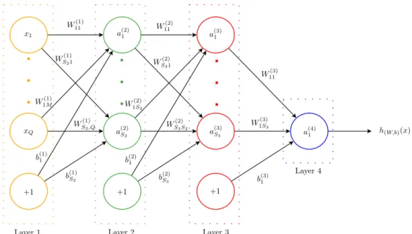
2.4.1 Artificial Neural Networks (ANNs) . . . 27
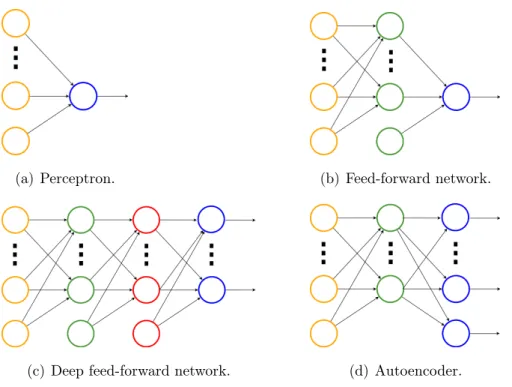
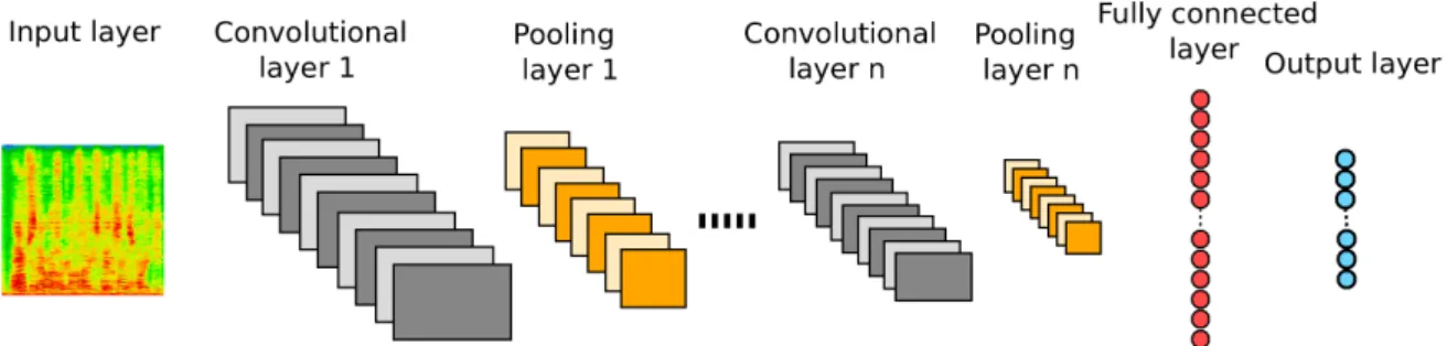
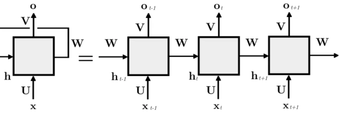
2.4.2 Main Types of Artificial Neural Networks . . . 32
2.5 Deep Learning for Speech Separation . . . 41
2.5.1 Applications of DNNs to Speech Separation . . . 41
2.5.2 Low-Level Features . . . 45
2.6 Room acoustic effects . . . 47
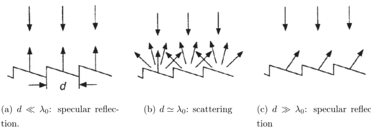
2.6.1 Acoustic reflections . . . 47
2.6.2 Room reverberation . . . 49
2.6.3 Deep learning for source localisation in reverberant environments 50 2.6.4 Deep learning for source separation in reverberant environments 51 2.7 Data sets . . . 52
2.7.1 RIRs data sets . . . 52
2.7.2 TIMIT . . . 54
2.7.3 Non-Speech Data set . . . 55
2.8 Evaluation Metrics . . . 55
2.8.1 Objective Metrics . . . 55
2.8.2 Perceptual-like Metrics . . . 55
2.9 Analysis of variance (ANOVA) . . . 56
2.10 Summary . . . 56
3 Speech and Noise Separation with Deep Neural Networks 59 3.1 Speech Separation with DNNs . . . 60
3.1.1 System Overview . . . 60 3.1.2 Proposed System . . . 60 3.1.3 Implementation . . . 63 3.1.4 Experiments . . . 65 3.1.5 Experimental Setup . . . 67 3.1.6 Experimental Results . . . 68
3.2 Dropout Algorithm Applied to DNNs for Speech Separation . . . 72
3.2.1 System Overview . . . 72
3.2.2 Proposed System . . . 72
3.2.3 Implementation . . . 73
3.2.4 Experimental Setup . . . 73
3.2.5 Experimental Results . . . 74
3.3 Speech-Noise Separation with DNNs . . . 75
3.3.1 System Overview . . . 76 3.3.2 Soft-Masks Generation . . . 76 3.3.3 Implementation . . . 77 3.3.4 Experimental Setup . . . 77 3.3.5 DOA Detection . . . 80 3.3.6 SDRs Evaluation . . . 83 3.4 Conclusions . . . 86
4 Speech Separation with Convolutional Neural Networks and Spatial Cues 89 4.1 Introduction . . . 89
4.2 Proposed System . . . 90
4.2.1 Contextual Frames Expansion . . . 91
4.2.2 Soft-Masks Construction . . . 92
CONTENTS v
4.3 Signal to Distortion Ratios (SDRs) Evaluation . . . 95
4.4 Conclusions . . . 99
5 DNNs based Speech Separation for B-format Recordings 101 5.1 Introduction . . . 101
5.2 Background . . . 102
5.2.1 Sound Pressure and its Acoustic Pressure Gradients . . . 102
5.2.2 Angular Feature . . . 104 5.3 Proposed Method . . . 105 5.3.1 Input Features . . . 105 5.3.2 The DNN Architectures . . . 107 5.3.3 Implementation . . . 109 5.4 Experiments . . . 110 5.4.1 B-format RIRs . . . 110 5.4.2 Experimental Setup . . . 111
5.4.3 Baselines and Performance Metrics . . . 112
5.4.4 Training . . . 112
5.5 Results and Analysis . . . 114
5.5.1 Masks Estimation . . . 114
5.5.2 Performance Evaluation . . . 116
5.5.3 ANOVA tests . . . 118
5.6 Conclusions . . . 121
6 Conclusions and Future Research 123 6.1 Conclusions . . . 123
6.1.1 Speech and Noise Separation from Binaural Mixtures with Deep Neural Networks . . . 124
6.1.2 Speech Separation with Convolutional Neural Networks and Spa-tial Cues . . . 125
6.1.3 DNNs based Speech Separation for B-format Recordings . . . . 125
6.2 Future Research . . . 127
Acronyms
AMS Amplitude Modulation Spectrogram ANOVA ANalysis Of VAriance
AVDL Audio-Visual Dictionary Learning
BiLSTM Bi-directional Long-Short Time Memory (BiLSTM) BRIR Binaural Room Impulse Response
BSS Blind Source Separation CapsNet Capsule Network
CASA Computational Auditory Scene Analysis cIRM Complex Ideal Ratio Mask
CNN Convolutional Neural Networks CS Compressed Sensing
CTF Convolutive Transfer Function
CVAE Conditional Variational AutoEncoder DOA Direction Of Arrival
DNN Deep Neural Network
DRR Direct-to-Reverberant Ratio
DUET Degenerate Unmixing Estimation Technique ETSAC Ellipsoid Tangent Sample Consensus
FCDNN Complex-Domain DNN
GFCC Gamma-tone Frequency Cepstral Coefficient GF Gamma-tone Feature
GF-TPS Gamma-tone Frequency Target Power Spectrum GCC Generalised Cross Correlation
GMM Gaussian Mixture Model GRU Gated Recurrent Unit HOA High-Order Ambisonics HMM Hidden Markov Model IBM Ideal Binary Mask
ICA Independent Component Analysis
ILD Interaural Level Difference IPD Interaural Phase Difference IRM Ideal Ratio Mask
ISTFT Inverse Short Time Fourier Transform ITD Interaural Time Difference
ITDG Initial Time Delay Gap IVA Independent Vector Analysis KL Kullback-Leibler
LOG-MAG Log-Spectral Magnitude LOG-MEL Log Mel-Spectrum LPS Log Power Spectrum LSTM Long-Short Term Memory
MFCC Mel-Frequency Cepstral Coefficient MLP Multi-Layer Perceptron
MNMF Multichannel NMF
MRCG Multi-Resolution Cochleagram MSE Mean Squared Error
MV Mixing Vector
MVAE Multi-channel Variational AutoEncoder NMF Non-negative Matrix Factorisation NTF Non-negative Tensor Factorisation OPS Overall Perceptual Score
PDF Probability Density Function
PESQ Perceptual Evaluation of Speech Quality PNCC Power-Normalised Spectral Coefficient PLP Perceptual Linear Prediction
PSM Phase Magnitude Mask
RASTA-PLP Relative Spectral Transform PLP RIR Room Impulse Response
RNN Recurrent Neural Network SA Signal Approximation SAR Signal to Artifacts Ratio SDR Signal to Distortion Ratio SGD Stochastic Gradient Descent SIR Signal to Interference Ratio SNR Signal to Noise Ratio
CONTENTS ix
STOI Short-Time Perceptual Intelligibility SVM Support Vector Machine
SMM Spectral Magnitude Mask TBM Target Binary Mask T-F Time-Frequency
Symbols
∗ Conjugation {•} Indicator function k•kF Frobenius norm | • | Absolute value × Multiplication ∠ Phase angle ∀ For all ∇ Gradient Element-wise product ⊗ Convolution PNi=1 Summation over discrete index i from 1to N
T Transpose
∂f
∂W Partial derivative of f with respect to W
f0(•) First order derivative of f(•)
M or(Mij) Matrix Mij or M(i, j) Element of a matrix s.t. Such that v Vector vi orv(i) Element of a vector A Mixing matrix
a(L) Activation function matrix for the L-th layer
a(iL) Activation function in the L-th layer for the i-th neuron
α Learning rate ¯
α Average room absorption coefficient
b or+1 Bias unit
b Bias vector
b(C) Bias vector of a memory cell of a LSTM xi
b(L) Bias vector for theL-th layer of a fully-connected network
b(f) Bias vector for the forget gate of a LSTM
b(o) Bias vector for the new memory state of a GRU
b(i) Bias vector for the input gate of a LSTM
b(o) Bias vector for the output gate of a LSTM
b(SLL) Bias unit connecting the SL-th neuron for the L-th layer of a
fully-connected network
BS Batch size
β Sparsity penalty term
c sound wave velocity when travelling through the air
Ct Internal recurrent state at the time stept of a LSTM
˜
Ct Candidate for the state of a memory cell at the time stept of a LSTM
C Complex domain
γ Phase
DE Euclidean distance
d Size of the irregularities of a surface
df(t) Linear correlation coefficient
δ(iL) Error term for the i-th neuron in theL-th layer ∆θ Angular difference between two DOAs
∆SDR Average improvement for the SDR estimation
eartif acts Artifacts error
einterf erence Interference error
enoise Noise error
Fcrit F-value critical for the ANOVA test
Fvalue F-value for the ANOVA test
F Number of frequency bins
f Frequency bin index in the Fourier domain
ft Forget gate at the stept of a LSTM
GLP
LP feature
Gx Sound pressure gradient along the xaxis in the Fourier domain
Gy Sound pressure gradient along the y axis in the Fourier domain
Gz Sound pressure gradient along the z axis in the Fourier domain
GLP
x LP feature for the xchannel
GLP
y LP feature for the y channel
g Sound pressure gradient
gx Sound pressure gradient along the xaxis
CONTENTS xiii
gz Sound pressure gradient along the z axis
Hr
x RIR along for x channel for the r-th sound source in the Fourier domain
Hyr RIR for for y channel for the r-th sound source in the Fourier domain
H0r RIR for the omni-directional channel for the r-th sound source in the Fourier domain
hr
0 RIR for the omni-directional channel for the r-th sound source
ht Hidden state at the step t for a RNN
h(tC) Hidden state of a memory cell at the step t of a LSTM
h(tf) Hidden state for the forget gate at the step t of a LSTM
h(th) Hidden state for the new memory state at the step t of a GRU
h(ti) Hidden state for the input gate at the step t of a LSTM
h(to) Hidden state for the output gate at the step t of a LSTM
h(tr) Hidden state for the reset gate at the step t of a GRU
h(tz) Hidden state for the update gate at the step t of a GRU ˜
ht New memory state at the time step t of a GRU
hrx RIR along for x channel for the r-th sound source
hr
y RIR for for y channel for the r-th sound source
hW,b(x) Output of a neuron given an input x
η Step size
IRMr Ideal Ratio Mask for the r-th sound source
IRMx Ideal Ratio Mask for the r-th sound source for the x channel
IRMy Ideal Ratio Mask for the r-th sound source for the y channel
i Imaginary unit
i Index of the neuron
it Input gate at the step t of a LSTM
J Number of DOAs and number of classes in the softmax classifier
J(•) Cost function
J Instantaneous intensity in the Fourier domain
j Index of the test set and the DOA
j Instantaneous intensity
K Number of neurons in the hidden layer
K Number of frequency bins fed into each DNN (resolution of each DNN)
L Number of layers of a fully-connected network
LB Left-back microphone
LF Left-front microphone
Lo Last layer of a DNN
`0 L-0 norm
`1 L-1 norm
`2 L-2 norm
λ Weight decay
λ0 Wavelength of a sound wave
RB Right-back microphone
RF Right-front microphone
M Number of training samples
Mtest Number of testing samples
Mr T-F masks of ther-th sound source
m or (m) Training sample
N Number of DNNs
Nf Number of features
NH Number of hidden layers
n DNN index
ot Output of the step t for a RNN and a LSTM
O DNN prediction
P Number of microphones
P0 Omni-directional sound pressure in the Fourier domain
pvalue p-value for the ANOVA test
p0 Omni-directional sound pressure in the Fourier domain
p(•) Probability
ρ Sparsity parameter ˆ
ρj Sparsity for thej-th neuron
ρ0 Density of the air
ϕ Three components of the sound mixture Φx Spectrogram of a mixture
Φx Spectrogram of a mixture for thex channel
Φy Spectrogram of a mixture for they channel
Q Gas temperature
Q Number of input neurons
R Number of sound sources
R Real domain
RT60 RT60of a room
r Sound source index
rt Reset gate at the time step t of a GRU
CONTENTS xv
Sr Spectrogram of a sound source in the Fourier domain
SL Number of hidden units in the L-th layer
Sr Spectrogram of the r-th sound source in the Fourier domain
Sr,x Sound source spectrogram of the r-th source for the x channel
Sr,y Sound source spectrogram of the r-th source for the y channel
Stot Total reflective surface of a room
s(˜t) Vector of independent sound signals at the time ˜t
sr Vector of the r-th sound source
σ Activation function
T Number of time frames
t Time frame index in the Fourier domain ˜
t Discrete time index
τ Number of contextual frames before and after τ0
τ0 Central contextual time frame
θ DOA
Θ Angular feature
θ DNN parameters
U Weight matrix of the input of the current state t of a RNN
U(G) Weight matrix for the input of the gate G of a LSTM or a GRU
u Unit vector pointing from the sensor to the source
V Weight of the output of the current state t of a RNN
Vtot Total volume of a room
v Acoustic particle velocity
vinc Incident sound wave
V Number of neurons inside a hidden layer
X Data matrix of observations
XL Left spectrogram of a mixture of sources
XR Right spectrogram of a mixture of sources
x Input tensor
x(˜t) Mixture of recorded microphone signals at the time ˜t
x(m) Input training set for the sample m
xt Input of the step t for a RNN
x(t,n) Input data for the t-th time frame fed into the n-th DNN
Yr Separated spectrogram of the r-th sound source
y(m) Ground-truth training set for the sample m
ytn Output of the softmax classifier at the time t for the n-th DNN
W(G) Weight matrix for the gate G of a LSTM
W(L) Weight matrix for the L-th layer ˜
W Whitening matrix
Wij(L) Weight for the L-th layer connecting thei-th and the j-th neurons
z Weighted sum of inputs for theL-th layer
Chapter 1
Introduction
Speech source separation aims to extract individual sources from mixtures of multiple sound sources, e.g. speech, noise and music. The problem of separating multiple sound sources from sound mixtures is also known as thecocktail party problem [1]: one can imagine a situation in which two friends are in a party, with loud music in the background and other people around talking simultaneously. Humans have an innate ability to separate speech and sounds in a sound mixture. However, this is not a trivial task for computers.
In this thesis, the problem of speech separation is studied, with a varying degree of complexity with respect to room reverberation, the number of speech sources and the number of microphones available for capturing the sources.
Conventionally, the problem is addressed using a variety of classical methods such as Computational Auditory Scene Analysis (CASA) [2, 3], Independent Component Analysis (ICA) [4, 5], Non-negative Matrix Factorisation (NMF) [6] and Expectation-Maximisation (E-M) algorithm [7], with the latter being used for finding maximum likelihood estimates of the parameters in a statistical model. Recently, deep learning techniques have been introduced for speech separation, showing improved performance over the classical techniques.
In this thesis, the state-of-the-art deep learning techniques are used to separate individual speech sources from mixtures of sound sources in real reverberant rooms. In Section 1.1, we present the motivations that led to this thesis work, by listing the issues that are yet to be solved and why they need to be solved. Our solutions are in Section 1.2, which contains the objectives and our ideas and the improvements achieved over previous works in the literature. In Section 1.3, a summary of the whole thesis is provided, including our novel contributions for addressing these problems.
1.1
Motivation
Addressing the speech separation problem will be beneficial to a variety of practical applications in real life, such as hearing aids [8], audio restoration [9] and abnormal speech detection on social media [10]. In hearing aids, speech separation techniques are used to help hearing-impaired people in improving the quality of their lives, by in-creasing the speech intelligibility and reducing the noise artifacts. In audio restoration, speech separation can be used to clean dated speech recordings from noise or other environmental sounds, which can severely affect the quality of such speech recordings. In abnormal (such as hate) speech detection, speech separation can be used to enhance the key words such as ‘evil’, ‘attack’, and ‘terrorist’ corrupted by noise, in order to prevent their negative spread on social media.
The main task of this thesis is to estimate one or more individual speech sources from mixtures of speech sources and/or noise. Real recordings are used, so the prob-lem studied is not just a mathematical model that emulates reality but represents a real application scenario, so the cases studied in this thesis can potentially have a high impact in the above mentioned practical applications. In addition, room reverberation and the effects of the room acoustics, that induces further complications to the sepa-ration problem will be considered. In this case, the speech sources are overlapped with acoustic reflections from room surfaces, so they are more difficult to separate com-pared to the case without room reverberation. In this thesis, recorded Room Impulse Responses (RIRs), representing the natural reverberation of a room, are used.
Early methods for speech separation include ICA [4, 5], CASA [3], NMF [6], and E-M algorithm [7]. However, their performance is limited for separating reverberant mixtures or for dealing with under-determined problems, where the number of sources is larger than the number of mixtures. Recently, deep learning techniques have shown to outperform classical methods for speech separation such as NMF [11, 12] and E-M [13], thus, this technique will be the focus of this thesis.
Several Deep Neural Networks (DNNs) architectures such as fully-connected net-works and Convolutional Neural Netnet-works (CNNs or ConvNets) [14], have been used for speech source separation. In particular, the single channel case, i.e. separat-ing multiple sources from a sseparat-ingle sound mixture, has been studied in several works [11, 12, 15–19]. However, when using a single microphone, the separation performance can be limited, as one can only resort to the spectral or temporal information, available in the single channel recording. To address this issue, we use multiple microphones to exploit the additional information from spatial cues, which can be obtained from multi-channel mixtures.
1.1. MOTIVATION 3
Many papers exist on binaural speech separation [13, 20–24], where two micro-phones are used for taking the recordings, often placed inside a dummy head in order to reproduce the cues available to human listeners. These works often involve record-ings inside reverberant rooms, where the early and late reflections behave like a noise source, thus increasing the complexity of the case studied.
Some of these methods only rely on the spatial information obtained by binaural microphones, resulting in limited separation quality. We address this limitation by introducing spectral features, such as the Log-Power Spectrogram (LPS) [25], which is particularly effective in the case of noisy speech separation. In addition, these methods do not exploit explicitly the contextual information from the neighbouring frames of a given time frame, even though the source location information changing with respect to time has been considered to certain extent. For this reason, we exploit thecontextual frames expansion technique, in order to improve the separation performance. We also explore CNN-based architectures for speech separation, which have shown to be more effective for single channel speech separation compared to fully-connected architectures [26–28].
The number of speech sources in the mixtures may vary and can exceed the number of microphones. Two-microphones perform well for separating mixtures of two speech sources, but other works [13] show that the separation performance degrades rapidly when the number of talkers is further increased. This suggests that more microphones need to be used in order to improve the separation quality.
Several works [29–35] attempt to overcome this limitation by recording the speech sources with multi-microphones or a microphone array, then introducing DNNs archi-tectures to perform speech separation. However, these works only rely on the sound pressure information, which is commonly used in speech separation.
Different from these works, a particular setup of SoundField microphone [36], called the B-format microphone has been exploited in other works [37–41], where the pressure gradient information is also used for speech separation, based on statistical methods such as Gaussian Mixture Model (GMM). However, when the number of talkers in-creases, GMM-based methods show limited separation performance.
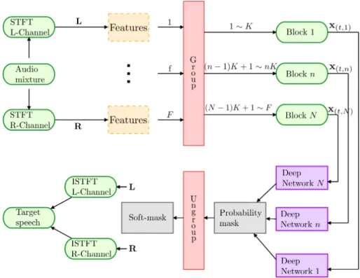
Some works [42–44] on speech separation show that DNNs based architectures can improve the separation quality compared to GMM-based techniques. For this reason, we will focus on the deep learning architectures, and examine their performance for B-format recordings using spatial and spectral features extracted from B-format mixtures, aiming to estimate the Time-Frequency (T-F) masks for multiple speech sources. A T-F mask, which is a matrix of T-F elements each indicating the occupation probability, is applied to the speech mixture matrix in the T-F domain to estimate a
given speech source.
In summary, the aim of the thesis is to further improve the performance of deep learning techniques for speech source separation, with a focus on binaural and B-format recordings, for different number of sources and a different level of room reverberation.
1.2
Objectives
There are three main specific objectives.
• We evaluate a recent baseline system [42] for binaural speech separation, which consists of fully-connected DNNs and further improve its performance by intro-ducing dropout [45, 46] and additional features such as the LPS.
• We study the potential of using data augmentation techniques to improve speech separation quality. In particular, we explore the use of contextual frames ex-pansion [17], by introducing the additional information from neighbouring time frames, before and after a given time frame.
• We study the potential of using deep learning for speech separation of B-format recordings obtained with a SoundField microphone [36], allowing the pressure gradient information to be exploited, in addition to the widely used acoustic pressure information. To our knowledge, this is the first work on deep learning for source separation applied to B-format recordings.
The work presented in this thesis may potentially be applied to several real-life cases, as introduced in Section 1.1. Our speech separation algorithms can be used to isolate the speech content of a talker in a noisy environment (e.g. a busy street) whose speech is corrupted by background noise or additional interfering talkers. As previously explained, this could be useful for speech detection from social media, e.g. for preventing the spread of hate messages on social media. Our work on binaural microphones can potentially be applied to hearing aids, by improving the speech en-hancement performance of the device, which is currently limited when the listener is not facing the direction of the talker. Being able to extend our experimental setup to the real-world scenario requires a generalisation of the test cases. For this reason, we tested our systems in the case of mixtures with up to four speech sources, which is possible where additional microphones are used, such as in the case of recordings obtained using the B-format microphone. We take into account the room acoustics, by adding a certain level of reverberation to speech mixtures used in our experiments. This takes our study closer to the everyday life scenario.
1.3. CONTRIBUTIONS AND THESIS ORGANISATION 5
1.3
Contributions and Thesis Organisation
This section summarises the main contributions of this thesis.
Chapter 3: Speech and Noise Separation from Binaural
Mix-tures with Deep Neural Networks
Earlier work in the literature has used the GMM framework to model the distri-bution of various cues at each T-F point of binaural mixtures, such as Mixing Vector (MV), Interaural Level Difference (ILD) and Interaural Phase Difference (IPD) [47]. More recently, other works started implementing DNNs for the estimation of T-F masks [13, 42, 48], showing that DNNs can achieve better performance compared to the GMMs technique used in [47].
However, the DNNs structures used are relatively basic and tend to over-fit with training data. The recently introduced dropout algorithm [45, 46], addresses this issue by removing a certain amount of neurons within the hidden layers, so that the DNNs can be better generalised and are less subject to overfitting. In Chapter 3, we introduce the dropout algorithm and compare the performance for different levels of dropout, including the case where no dropout is applied.
In [13], only spatial cues such as MV, ILD and IPD are used for the DNNs training. The above spatial features become less effective for speech-noise scenarios where the target speech is often masked by the background noise in adverse conditions. Moreover, if the environment is reverberant, the performance of the existing method degrades radically.
Speech sources and background noise often bear essential differences in their spec-tral structure. Specspec-tral features, such as LPS, have been proved useful as DNN input to extract target speech sources corrupted by noise from monaural recordings [17, 49], which provide complementary information to the spatial cues. In Chapter 3, we will examine the use of spectral features, such as LPS, to enhance the performance of the baseline system that was based on the use of binaural features. We will also study the case where different types of noise sources at different levels of SNRs are used as an interferer for a target speech in rooms with different reverberation levels.
To summarise, this chapter studies three main problems:
1. Speech-speech separation, by using a system of DNNs, which is trained by using only the binaural cues such as MV, ILD and IPD. Each DNN terminates with a softmax layer, which is used to estimate the probabilities for each speech source to come from a given Direction Of Arrival (DOA). This information is used to
generate the T-F masks, in order to separate the target speech.
2. Speech-speech separation by introducing the dropout algorithm to the above system, and compared to the case without using the dropout.
3. Speech-noise separation, where a similar system using the dropout algorithm and binaural features is used, and compared with the additional use of the LPS feature, for the case in which the interferer is a noise source.
This work was presented in the following publications:
• A. Zermini, Y. Yu, Y. Xu, W. Wang, and M. D. Plumbley, “Deep neural network based audio source separation,” in Proceedings of the 11th International IMA International Conference on Mathematics in Signal Processing, 2016.
• A. Zermini, W. Wang, Q. Kong, Y. Xu, and M. D. Plumbley “Audio source separation with deep neural networks using the dropout algorithm,” in Proceed-ings of the Signal Processing with Adaptive Sparse Structured Representations (SPARS) 2017, 05-08 Jun 2017, Lisbon, Portugal.
• A. Zermini, Q. Liu, Y. Xu, M. D. Plumbley, D. Betts, and W. Wang, “Binaural and log-power spectra features with deep neural networks for speech-noise sepa-ration,” in IEEE 19th International Workshop on Multimedia Signal Processing, October 2017.
Chapter 4: Speech Separation with Convolutional Neural
Net-works and Spatial Cues
The problem of estimating a speech source from a mixture of talkers is particularly challenging for the case where some level of reverberation is introduced, especially when only two microphones are employed for the recordings.
In the literature, the vast majority of papers are based on fully-connected networks, which are relatively easy to implement due to their simple architectures, but show some limitations on the separation performance.
In [13], several rooms with different levels of reverberation are used, where the target speech is separated by using a T-F mask. A system of DNNs is trained by using binaural spatial cues as input. However, the level of reverberation in the speech mixtures is shown to affect the separation performance, in particular when the training room used is different from the room used in the testing set. In a similar way, other works [20–22,50] implement fully-connected networks, fed with spatial features in order to estimate the T-F masks.
More recently, other neural network structures, such as CNNs [51], have become more popular in deep learning. In particular, some works [26–28] suggest how the
in-1.3. CONTRIBUTIONS AND THESIS ORGANISATION 7
troduction of CNNs improves the separation performance compared to fully-connected DNNs. However, CNNs have more complex architectures compared to fully-connected DNNs and require a more appropriate choice of parameters, in order to achieve an overall improvement.
With this in mind, in this chapter, we aim to upgrade the system of DNNs intro-duced in [13] to a system based on CNNs, in order to exploit the increased computa-tional power available in modern GPUs, allowing for a better DOA estimation and, consequently, generating more accurate T-F masks for source separation.
In order to better generalise the trained CNNs and improve the separation per-formance, we also explore additional techniques, such as the dropout technique, as studied in Chapter 3. In this chapter, we apply the dropout algorithm to the final dense layer of each CNN, aiming to better generalise the trained architecture.
In feed-forward architectures, each time frame in a feature is fed without giving a proper contextual information, meaning that each frame is fed into the DNN without taking into account what the feature contains in the neighbouring time frames. In fact, speech signals have strong temporal correlation, so giving to the CNNs a wider view on the input features allows for a better separation quality. This technique, called contextual frames expansion [17], has been already used in different cases, such as [17] for speech enhancement and more recently in [24] for speech separation, showing improved separation performance. However, we use this technique for separating two talkers for the case of recordings in different reverberant rooms, aiming for a better adaptation of the trained CNNs. More specifically, we refer to the ‘mismatched’ case when each CNN is trained with speech sources recorded in a different room from the one used for the test samples. This case is particularly challenging, and requires additional data in order to better adapt the CNNs system to an unseen level of reverberation. For this purpose, we test different amounts of neighbouring time-frames and compare their performance.
The improved system of CNNs has been compared to a baseline system of analogous fully-connected DNNs, which has been introduced in Chapter 3. In order to make the comparison as accurate as possible, the performance of the novel system is tested in rooms with the same or a different level of reverberation with respect to the training room.
This work resulted in a publication in a recent conference:
• A. Zermini, Q. Kong, Y. Xu, M. D. Plumbley, and W. Wang, “Improving rever-berant speech separation with binaural cues using temporal context and convo-lutional neural networks,” in Proceedings of the 14th International Conference on Latent Variable Analysis and Signal Separation, Y. Deville, S. Gannot, R.
Mason, M. D. Plumbley, and D. Ward, Eds. Springer International Publishing, 2018.
Chapter 5: DNNs based Speech Separation for B-format
record-ings
While the single-channel and binaural source separation are the most studied cases for DNN-based speech separation, in literature little attention has been given to the multi-channel case. However, for the multi-channel case the information provided by additional microphones can be exploited, which can potentially improve the quality of the estimated speech compared to the monaural and binaural cases.
The multi-channel case has been studied with different types of microphone arrays, differing in the number of microphones used and their placement in space. A six-channels microphone array mounted on a tablet is used in [30], where a framework of DNNs combined with the E-M algorithm is used to directly estimate the sources in single-talker noisy audio recordings. However, besides the relatively low quality of the microphones used, this method has been tested on mixtures of only two sources, generated by artificially mixing clean speech and different types of background noise [29].
The more common four-channels case is studied in [31], where the output of High-Order Ambisonics (HOA) format is used as an input to a Long-Short Term Memory (LSTM) network [52], for the T-F mask estimation from the mixtures of two noise-corrupted talkers. The main limitation of this study is the assumption of the DOAs of the sources being known, in order to provide reliable estimations. Microphone arrays with four channels are also used in [53], where a subspace method is exploited for the DOA estimation, which is then used for source separation. However, the performance of these separation systems also degrades with the increase in the number of talkers.
More recently, DNNs-based techniques have been used in combination with classic techniques. More specifically, ICA [30, 32, 33], beamforming [34] and GMMs [35]. However, these methods show limitations for highly reverberant environments [33], or employ a large number of microphones [34], or have been tested only for low-quality recordings [35].
The main limitation of these works, is that they are solely based on the sound pressure information, like the vast majority of papers on single, binaural and multi-channel cases. Recently, the information from the acoustic pressure gradients has been exploited for a series of other works [37–41]. The acoustic pressure gradients can be recorded by using microphone arrays, such as a SoundField system [36]. More
1.3. CONTRIBUTIONS AND THESIS ORGANISATION 9
specifically, a particular type of SoundField system has been used, namely the B-format microphone, which contains a densely-distributed array of four microphones. One microphone is used to gather the information of the sound pressure, while the other three, oriented along the x-y-z axes, can measure the pressure gradient along each axis.
A B-format microphone has been used in [37, 39–41], where GMM-based clustering methods are used to separate multiple speech sources. However, these works show some limitations in terms of the number of talkers considered for the mixtures [37], limited number of metrics used for the performance evaluation [39] or lack of evaluation for the case of closely-spaced sources [40, 41].
In this chapter, we study the potential of using deep learning techniques for speech separation for B-format recordings. To our knowledge, the literature lacks of DNNs based methods for B-format microphone recordings, with the only exception of [54], where deep learning is exploited to generate ambisonics using both audio and visual cues for a virtual reality application. However, deep learning techniques have been previously used in combination with multi-channel microphone recordings for speech enhancement and recognition [55–57].
Using the correct DNN structure is important in supervised speech separation. While more advanced DNNs structures have shown improved performance over simpler fully-connected structures [24, 58], e.g. Multi Layer Perceptrons (MLPs) [59], other works [11] suggest that the difference between e.g Recurrent Neural Networks (RNNs) and MLPs are small. For this reason, we want to test a MLP structure, because it is straightforward to implement and has already proved to achieve satisfactory separation performance in speech separation with training by regression [11, 15, 16] and compare it with a CNN architecture, which is shown to improve the performance by fully-connected structures in several works [26–28].
When training a DNN, choosing appropriate input features is crucial for separa-tion performance. Deep learning techniques often struggle when the mixtures contain several speech sources, especially when these are closely located within space. For this reason, using spatial features only may not be sufficient in achieving a good separation performance. Some papers on binaural speech separation [24, 60] suggest that adding spectral features on top of binaural features can improve the separation quality of a DNN on speech mixtures. Following the same idea, we train a DNN architecture by using the spatial information of an angular feature [39] on top of the spectral LPS feature for B-format microphone recordings. For the DNN output, we chose Ideal Ra-tio Masks (IRMs) as ground-truth when training the DNN, which are shown in [12] to achieve better separation performance compared to other type of Fourier-domain
targets when training an MLP, such as binary masks. In addition, in order to better generalise the trained DNNs, other techniques such as the dropout algorithm and the contextual frames expansion, studied in Chapters 3 and 4, will also be incorporated and evaluated.
This work has been recently submitted to IEEE Journal of Selected Topics in Signal Processing.
Chapter 2
Literature Survey
2.1
Introduction
This chapter provides literature review of the existing methods for speech separation. In Section 2.2, the problem of speech source separation is introduced, where the prob-lem is formulated in terms of the number of sources and microphones, the presence of room reverberation and the mixing model.
Section 2.3 contains an overview of the main classical techniques used for speech separation in the literature, e.g. ICA, CASA, NMF, sparse representation and dictio-nary learning. The main methodology used in this thesis, deep learning, is introduced in Section 2.4. In Section 2.4.1, the main types of network structures are discussed, starting from the very simple perceptron structure to the latest architectures, such as Capsule Networks (CapsNets) [61] and Generative Adversarial Neural Networks (GANs) [62]. In Section 2.5.1, a number of existing works on applying deep learning techniques to speech separation are discussed and categorised, based on the number of microphones available for the recordings: monaural, binaural and multi-channel cases. The input features and training targets often used, are discussed in Section 2.5.2 and Section 2.2.1, respectively. In Section 2.6 we will explain how the room acoustic phenomena affect the reverberation of indoor environments, while in Section 2.7 we introduce the data sets used in this thesis. Finally, in Section 2.8, we present the metrics that will be used to evaluate the separation performance. Finally, Section 2.10 briefly summarises this chapter.
2.2
Problem Formulation
The speech separation problem has been considered classically under the framework ofBlind Source Separation (BSS), which aims to separate the sources with no (or very
little) information about the sources and mixing channels.
In the case of Rsound sources, the general problem (without noise) to be solved is
x(˜t) =As(˜t) (2.1) wheres(˜t) = (s1(˜t). . . sR(˜t))T contains theRindependent source signals at the discrete
time index˜t, x(˜t) = (x1(˜t). . . xP(˜t))T contains theP recorded microphone signals and
A is the so-called mixing matrix, whose dimension is P ×R. In general, both A and
s are unknown, and need to be estimated, givenx(˜t).
Taking into account the number of microphones and sources, three scenarios can be distinguished:
• Over-determined case. The number of microphones is larger than the number of sources (R < P).
• Determined case. The number of microphones is equal to the number of sources (R=P).
• Under-determined case. The number of sources is larger than the number of microphones (R > P). In many situations, the number of sound sources is not known and may be greater than the number of mixtures. The separation of under-determined mixtures requires additional assumptions on the source signals than in the over-determined case such as sparsity, in order to reduce the possible solutions in the solutions space.
Depending on the level of surface reflections in an acoustic environment, three types of mixtures can be distinguished:
• Instantaneous mixtures. Each microphone records a signal which is a linear combination of the source signals. In other words,A is a scalar matrix.
• Anechoic mixtures. Each microphone picks up the mixtures of the direct sound from the sources. A is a scalar matrix and s(˜t)→s(˜t−δ), whereδ is the time taken for the source to reach the microphone.
• Convolutive mixtures. Room reverberation affects the audio collected by micro-phones, leading to superposition of direct sound sources and time-delayed source component due to room reflections. In this case, A is a matrix of filters. Room reflections also depend on the experimental methodology employed. Other fac-tors to take into account are measurement noise (electrical and acoustical), room geometry, acoustic treatment, source directivity, air flow, temperature, humidity, homogeneity and even the presence of people and other scatterers [63].
Depending on whether the measurement process is linear, we have:
• Linear case. The mixture is a linear combination of the sources as represented by model (2.1).
2.2. PROBLEM FORMULATION 13
• Non-linear case. The relation between x and s is characterised by a non-linear function, such as x=exp(s), whereexp(•) is an exponential function.
In this thesis, the determined and under-determined cases will be studied. In partic-ular, we study the binaural case whereP = 2, and the source separation for B-format mixtures whereP = 4. In both cases, convolutive linear mixtures are considered.
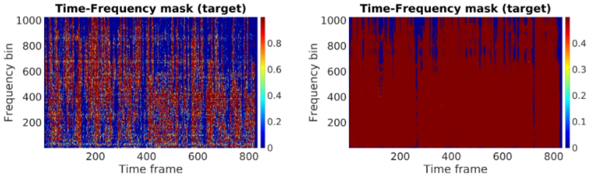
Our method consists in the estimation of the T-F mask, which is a matrix whose elements are in the range [0,1]. The target speech can be estimated by multiplying element-wise the speech mixture spectrogram with the T-F mask. We assume the number of sources is known, which is the same as the number of T-F masks to be estimated. The number of sources to estimate is R = 1 for Chapter 3 and Chapter 4, while it is eitherR = 3 or R= 4 in Chapter 5. In all these cases, we assume that the sources have a high Direct-to-Reverberant Ratio (DRR), which represents the ratio between the energy of the direct sound and the reflections.
2.2.1
The goal of speech separation
The goal of speech separation is to separate target speech from background interference [64]. In the history of speech separation, several different types of targets have been used. Here, we describe the most commonly used targets.
Ideal Binary Mask (IBM)
Ideal Binary Mask (IBM) is a popular choice of training target used for training the neural networks [65]. Inspired by auditory masking in human hearing [66] and the exclusive allocation principle in auditory scene analysis [67], the IBM is defined as [68]
IBM(t, f) = 1 if STSI((t,ft,f)) >1 0 otherwise (2.2)
where ST = (ST(t, f)) and SI = (SI(t, f)) indicate, respectively, the target and
in-terferer spectrograms. The IBM labels each T-F unit either as target-dominant or interferer-dominant. In [69] it is shown that, although the IBM improves speech in-telligibility in noisy condition, the separated speech is unnatural. Similar results are obtained in [70] on noise-corrupted speech separation, showing that IBM improves speech intelligibility but not speech quality. However, in [71] it is argued that the IBM corresponds closely to auditory masking, i.e. a sound is either masked or not. If we define the noisy speech as
given a mask M, the clean speech can be reconstructed from noisy speech [72]
ST =M∗Y (2.4)
where ST and Y are the Short-Time Fourier Transform (STFT) of clean speech and
noisy speech respectively, and the operator ∗ is the element-wise complex multiplica-tion.
Target Binary Mask (TBM)
Different from the IBM, the Target Binary Mask (TBM) is calculated from the target sound only and therefore is independent of the interferer sound:
T BM(t, f) = 1 if STr((ft,f)) >1 0 otherwise (2.5)
where r = (r(f)) is the long-term average spectrum of the target speech. The TBM has been used as a training target in [73, 74], showing better performance than the IBM in noisy speech mixtures, but degrading the intelligibility of clean speech.
Ideal Ratio Mask (IRM)
The Ideal Ratio Mask (IRM) is another popularly used training target, defined as
IRM(t, f) = ST(t, f)
ST(t, f) +SI(t, f)
(2.6)
In [75] the IRM is considered as a closer match to psycho-physical and perceptual mechanisms than IBM, because there should be some kind of sensory threshold in listeners, even though the perception does depend on the individual listener. In [76] it is proven that the IRM achieves higher SNR gains compared to the IBM, even if the SNR gains are quite close. In [70], the IRM improves both speech intelligibility and speech quality over the IBM under the assumption that clean speech is independent from noise. However, there are some cases in which it is better to choose the IBM over IRM for its simpler estimation [76]. The IRMs have been employed as a training target in [48].
Spectral Magnitude Mask (SMM)
The Spectral Magnitude Mask (SMM, also called FFT-MASK) is defined as
SM M(t, f) = |S(t, f)|
2.2. PROBLEM FORMULATION 15
where|S(t, f)|and |Y(t, f)|are, respectively, the spectrogram magnitudes of the clean speech and noisy speech. Different from the IRM, the SMM is not upper-bounded by 1. To obtain the separated speech, the SMM is applied to the spectral magnitudes of noisy speech, then the separated speech is re-synthesised with the phases of noisy speech (or an estimate of clean speech phases). An example about how this mask has been used can be found in [12], where the SMM is shown to perform better perceptually than binary masks such as IRM and TBM.
Phase-Sensitive Mask (PSM)
By including the phase difference between the clean speech and the noisy speech, i.e.
γ, the Phase-Sensitive Mask (PSM) can be defined by multiplying the SMM bycosγ
as follows [77]:
P SM(t, f) = |S(t, f)|
|Y(t, f)|cosγ (2.8)
The work in [78] shows that a better clean speech estimation can be achieved by using the PSM instead of the SMM. In [70], it was shown the PSM improves speech intelligibility and speech quality significantly, outperforming other training targets, e.g. IBM, IRM and cIRM.
Complex Ideal Ratio Mask (cIRM)
The Complex Ideal Ratio Mask (cIRM) is defined with both real and imaginary com-ponents (below the operations are meant to be element-wise):
cIRM= YrSr+YiSi
Y2r+Y2i +i
YrSi+YiSr
Y2r+Y2i (2.9)
where Yr and Sr are the real parts of Y and S, while Yi and Si are the imaginary
part.
The advantage of the cIRM over the PSM is that it is able to exploit the phase information of the spectrum, which is often ignored by the majority of source sepa-ration approaches. The cIRM has been used in [79], where a Complex-Domain DNN (FCDNN) is used to estimate complex STFT coefficients, showing higher SDR, SIR and PESQ compared to other baseline approaches, where IRM is used as a training target.
Gammatone Frequency Target Power Spectrum (GF-TPS)
The Gammatone Frequency Target Power Spectrum (GF-TPS) [12] is defined as the power of the cochleagram response of the clean speech. Unlike the TBM, which is de-fined on a spectrogram, this target is dede-fined on a cochleagram based on a gammatone
filterbank [64] and has an advantage over other target masks in that, once the GF-TPS is estimated, it can be easily converted to the separated speech waveform through the cochleagram inversion [3].
Signal Approximation (SA)
The Signal Approximation (SA) is generated by minimising the difference between the spectral magnitude of clean speech and that of estimated speech. In other words, the DNN is trained so that the estimated mask, when applied to the mixture, leads to the best approximation of the reference signal [11, 80]:
SA(t, f) = [M(t, f)|Y(t, f)| − |S(t, f)|]2 (2.10) where M= (M(t, f)) is the mask estimated. This approach has been used in [80] for speech separation using a three hidden layer DNN. This study also compares all the above mentioned T-F masks as targets, suggesting that the IRM and the SMM can achieve the best separation performance for speech separation.
2.3
Classical Methods
Several techniques have been successfully applied to the audio source separation prob-lem. For example, binary and soft time-frequency masking [81], have been applied to the sound mixture in the time-frequency domain. ICA [4, 5] is based on the statistical independence between the sound sources and works for over-determined or determined mixtures, while CASA [3] tackles the problem from a human perception point of view. NMF [6,82] factorises the mixture spectrogram into a dictionary of source components weighted by activation coefficients and works well in the case of unsupervised monau-ral source separation. Dictionary learning based sparse representation technique [83] has been used for under-determined sound separation.
The following sub-sections will briefly present several main approaches that have been developed for speech separation.
2.3.1
Independent Component Analysis (ICA)
In Independent component analysis (ICA) [4, 5], each mixture xand sources in (2.1), are assumed to be a random variable, with zero mean (otherwise they can always be centred by subtracting the sample mean). Moreover, the sources s are assumed to be statistically independent, which means that the following relation on the probabilities
2.3. CLASSICAL METHODS 17
holds for the two variables yi, yj:
p(yi, yj) = p(yi)p(yj) (2.11)
where p indicates the joint density function. When the two variables are Gaussian distributed, p(yi, yj) would be itself Gaussian, therefore it would not contain any
in-formation on the directions of the columns of the mixing matrixA: this implies that the ICA model cannot be used for separating multiple Gaussian sources.
Two main problems arise when using the ICA techniques: considering that both
A and s are unknown, it is impossible to estimate the variances of the independent components and their order. While on one hand ICA guarantees unique solutions subject to scale and permutation ambiguities, the weak point of ICA-based techniques is that, in order to be effective, it is necessary to first estimate the number of unknown sources from the mixture before performing source separation. Moreover, ICA is not suitable for sources which are mutually dependent [84].
The problem of separating mixed speech signals using ICA has been widely in-vestigated. Early papers [85, 86] attempt to recover multiple unknown source signals from multiple observed signals that are mixtures of the sources. However, the method in [86] is successful in those cases where [85] fails, e.g. for weak signals in a high level of noise. In more recent papers, such as [87], ICA is applied to convolutive mixtures of two speech sources, picked-up by two-microphones. The sources are extracted one by one in a decreasing order of negentropy from the mixed signal. An interesting work [88] presents a mathematical framework that explains when and how standard ICA can perform source separation from a single sensor. A novel likelihood ratio function is de-veloped to measure the confidence toward independence in [89], which achieves better speech recognition performance compared to other ICA-based methods. A different approach consists in using ICA techniques for the estimation of Ideal Binary Masks (IBMs) in [90, 91]. More specifically, in [90], a method for instantaneous mixing model is proposed, which assumes closely spaced microphones. IBMs estimated from the outputs of an ICA algorithm are used to extract an arbitrary number of speech sig-nals. In [91], ICA is used to estimate the IBMs for separating the source signals from two-microphones recordings of convolutive speech mixtures, but includes an additional step, which introduces cepstral smoothing, in order to reduce musical noise caused by the T-F masking. Other works [92] aim for a lower computational complexity and a faster convergence compared to standard ICA methods [5], where a target speech is extracted and recognised from noisy stereo mixtures.
An efficient and popular algorithm for ICA, named FastICA [5], is employed in several works [93–97], offering fast convergence, guaranteed global convergence for
cer-tain mixing conditions and contrasts, and robustness in presence of noise. Convolutive mixtures are separated in [93] by using the FastICA algorithm. This algorithm com-bines multi-channel whitening with fixed-point iterations, which allows the sources to be reconstructed as they appear in the observed mixtures. In [94], an enhanced FastICA is employed, showing less artifacts compared to the ICA method in [87]. A different approach is followed in [95], where ICA is used for identifying the active com-ponents of HMMs. The FastICA algorithm in [5] is here used to build independent voice space for talker and environment adaptation. The work in [96] is based on the maximisation of non-Gaussianity technique using Gradient ICA algorithm and Fas-tICA algorithm, then compares the results of both methods. While FasFas-tICA needs less execution time compared to Gradient ICA, the latter provides a higher efficiency in separating speech signals. FastICA is also combined with sparse component analysis in a recent paper [97], and applied to over and under-determined mixtures.
2.3.2
Computational Auditory Scene Analysis (CASA)
InComputational Auditory Scene Analysis (CASA) [3] the task is to separate mixtures of sound sources like human listeners do. In the same way in which an image is analysed and processed as a whole by sensing the single features, such as edges, textures and colours, the sound reaching the human ear is subject to Auditory Scene Analysis (ASA) [67].
A standard CASA system consists of four stages [3]:
1. Peripheral analysis: the input signal is processed using an auditory model, resulting in a cochleagram (a T-F representation).
2. Auditory features extraction: some features are generated.
3. Segmentation: the system generates a collection of segments or contiguous re-gions in a cochleagram.
4. Grouping: those segments which are likely to come from the same source are grouped into a perceptual structure, called stream, corresponding to how the source is mentally perceived by the listener.
CASA attempts to construct a machine that approaches human performance in ASA by using one or two microphones recordings of the acoustic scene, in order to extract individual source streams. A typical example in CASA aims to estimate an ideal time-frequency mask, built e.g. by using a model of peripheral auditory system called cochleagram, which emulates the human frequency selectivity. CASA is one of the first attempts to imitate the human auditory system for the purpose of creating an audio source separation system [98, 99].
2.3. CLASSICAL METHODS 19
Several works can be found in the literature, where CASA is applied to voiced and unvoiced speech separation. Some early works on CASA can be found in [100–102]. In particular, in [100] the separation algorithm determines the pitch period of each sound source, then a Markov model is used to determine the number of sounds present and the type of each source. The amplitude of each source is determined and, at last, a waveform of the separated output is re-synthesised. The work in [101] describes a multi-stage architecture for early auditory processing. The input sound is transformed into a map of neural firings in the cochlea, then cues are extracted from the cochlear image. The model groups these cues into single sound events, which are then grouped into sound sources. The model presented in [102] decomposes the signal into a series of T-F regions, then looks for coherent subsets of auditory objects, with a final grouping stage.
The residue-driven architecture is introduced in [103], which consists of an event-detector, which calculates the residue by subtracting the predicted input from the actual input, a tracer-generator, which extracts an auditory stream from the residue and returns a predicted input for the next time frame. The work in [104] introduces a multi-agent approach for sound stream segregation. Sound streams are first extracted from a mixture of sounds, and then some sound stream is selected. Following these works, in [105] the direction information of the sources is used to extract fundamental frequencies of individual harmonic sounds. Sound source directions and fundamental frequencies are used for sequential grouping of harmonic sounds.
A CASA model is the one studied in [65], where a multi-stage system that per-forms pitch estimation, is used for monaural speech segregation. This work was then improved in [106] by the same authors, where a tandem algorithm performs pitch es-timation of a target speech and segregation of voiced portions of target speech jointly and iteratively. A CASA system based on the model in [65] is guided by a metric called Objective Quality Assessment of Speech (OQAS) in [107] for monaural speech separation, increasing the accuracy of pitch estimation and, as a result, the separa-tion quality. In [108] the authors apply shape analysis techniques, such as labelling and distance functions, to complement discontinuous or missing auditory elements in speech signals and improve the performance of the CASA-based speech separation sys-tem. This technique improves the performance of the original CASA algorithm in [3]. In [109], the algorithm first classifies the T-F units, which are grouped together, and then detects amplitude modulation rates for the separation of monaural speech mix-tures. In this work, initial segments only consist of resolved T-F units satisfying the time continuity and cross-channel constraints, solving the issue in [65] of unresolved units being assigned to initial segments. Unlike [65, 107], which deal with voiced
seg-regation, in a more recent paper [110], the problem of unvoiced speech segregation in monaural recordings from non-speech interference is studied. Starting from unvoiced speech with non-speech interference, the system removes estimated voiced speech, and the periodic part of interference, then noise energy in unvoiced intervals is estimated and unvoiced speech segregation is performed. Classic CASA methods [3] are also improved in [111] by detecting pitch contours and assigning them to individual speech sources. Moreover, the method assumes that sound signals are not necessarily all-voiced speech. Pitch frequencies are detected, grouped, separated and missing pitch frequencies, caused by the stronger talker masking the weaker talker, are separated, in order to separate two speech sources from a mixture. The work carried out in [112], attempts to separate both the voiced and unvoiced target speech simultaneously from non-stationary monaural interfering sources by combining CASA with Max Vector Quantisation Model (MAXVQ) to infer the mask, whose choice is motivated by ob-serving that the log-energy in a narrow band of a mixture corresponds to the maximum of the individual logarithmic energy in that band. In [113], the problem of speech sep-aration is studied in the presence of either another speech source or noise by using classic CASA techniques to estimate an IBM. Different from the previously mentioned methods, weak assumptions are made about the various sound sources in the mixture and the features used are the Gammatone Feature (GF) and a cochleagram derived from Gamma-tone Frequency Cepstral Coefficients (GFCCs). GFCCs are also used in [114], which combines CASA and deep learning for monaural speech separation, where a DNN is used as a classifier to estimate the IBMs.
Current CASA techniques are limited by pitch estimation errors and residual noise. In particular, CASA-based methods have problems in separating instruments playing in the same pitch-range into different streams.
2.3.3
Non-negative Matrix Factorisation (NMF)
Non-negative Matrix Factorisation (NMF) aims to decompose a non-negative matrix
X ∈ RR×T into the multiplication of two non-negative matrices A ∈
RR×G and S ∈ RG×T as follows [6, 82]
X'AS (2.12)
In audio source separation, X = (Xrt) is a data matrix of observations for the r-th
source at the t-th sample,A = (Arg) a mixing matrix, and S= (Sgt)a source matrix,
where A and S are non-negative. In order to do this, it is necessary to use a cost-functionJE that quantifies the quality of the approximation. For example, considering
2.3. CLASSICAL METHODS 21
equation (2.1), the Euclidean distance
JE =DE(X;AS) = 1 2 X rt (Xrt−(AS)rt) 2 (2.13)
is one of the most commonly used cost-functions, whereris the source index andt the time index. By applying a simple descent step forS, this can be updated according to
S ←S−η∂JE
∂S (2.14)
or, in terms of elements,
srt←srt−ηrt
∂JE
∂srt
(2.15)
whereη is a small update factor known as step size.
Besides the Euclidean distance, it is possible to introduce additional constraints in the cost-function. A few of these cost-functions, like the extended Simultaneous Multiplicative Algebraic Reconstruction Technique (SMART), are presented in [115] and are able to achieve an improved efficiency and convergence rate.
In [116], NMF is used to decompose a spectrogram into a matrix in the frequency domain i.e. notes, and their location along time. The system is tested on both artifi-cially mixed audio and real musical recordings. Despite the good performance in terms of signal to noise ratio (SNR), the method proposed is computationally expensive be-cause it requires the phase information to be recovered through statistical inference. In fact, the phase information is not included in non-negative matrices. Moreover, the performance strongly depends on the number of bases used in the model.
In order to address this issue, other authors [117] expanded the classic NMF into complex NMF:
Xrt=
X
g
ArgSgteiφgrt (2.16)
However, this approach is not exactly a standard NMF because, apart from the non-negative matrices A and S, the third term on the right hand side (RHS) of equation (2.16), containing φgrt, is a complex tensor. The advantage of this method over the
classic NMF, is the possibility to process also the phase information, contained in the complex tensor φgrt. A more general extension of the NMF from matrices to tensors
is theNon-negative Tensor Factorisation (NTF), which has been studied in [118]. The main advantage of using NMF over methods such as ICA is that sources can be recovered without any prior knowledge about the mean and variance of the sources. However, NMF is algorithmically complex to implement and convergence can be slow.
Moreover, using NMF leads to non-unique solutions. Introducing the non-negativity constraint may not be sufficient to achieve sparseness in some situations, which has to be enforced by adding penalty terms to the cost-function [119].
With regard to speech separation, a relevant paper is [120], where a cross-coherence penalty is incorporated using a regularised NMF cost-function to learn discriminative and reconstructive dictionaries, followed by another work by the same authors [121], where a prior likelihood term is added to the NMF cost-function in order to encourage the log-normalised gain vectors of the NMF solution to increase their likelihood under a prior GMM. Standard supervised NMF methods show limited performance in min-imising the mismatch between the optimisation objective used to train the dictionaries and that is used to perform the actual estimation at testing time, in particular when speech and noise signals are of similar nature. For this reason, the work in [122] aims in matching the optimisation objective used at the training and testing stages. In [123], discriminative training of the NMF basis functions is used, like in [120], but this method has an additional training-time optimisation of the reconstruction of the basis functions. In [124], a regularisation term is added to the cost-function to overcome the limitation in standard NMF, where each frame is considered as an independent obser-vation. A recent work [125] combines unsupervised dictionary learning via NMF with spatial localisation by using the Generalised Cross Correlation (GCC) method. The advantage of this method is that no prior knowledge of sources or mixing conditions is required, as well as no training set of isolated sources or acoustic information.
Latest NMF-based methods employ deep learning techniques under the name of deep-NMF for speech separation, in works such as [126–129]. The works in [126, 127] improve the separation results over traditional NMF methods. In particular, deep-NMF is shown to outperform deep feed-forward networks for speech separation using fewer trainable parameters [126]. This problem is further studied in [129], where recurrence between the NMF coefficients of adjacent frames is exploited. The work in [128] improves previous two-stage approaches by combining T-F masking with NMF reconstruction [130], by taking into account mask estimation error. DNNs have also been applied to speech enhancement in [131], where the coding vectors of the NMF algorithm are estimated by using DNNs, improving traditional NMF methods, and [132], using a DNN-HMM approach to NMF.
2.3.4
Sparse Representation and Dictionary Learning
Sparse representation, represents a mixture signal in terms of a small number of active elements chosen out of a larger set [133]. More specifically, a sparse array has most elements set to zero. With the term dictionary learning we refer to the simultaneous
2.3. CLASSICAL METHODS 23
search for both dictionary and sparse representations of a set of training signals [134]. In sparse representation any coefficient is assumed to have only a small probability of being far from zero [135]. For example, if a musical piece is created by playing only a small number of notes on a 88 keys piano (such as a chord succession), with pitches active at a certain time, it is very straightforward to introduce the concept of sparsity just by thinking that, at a very specific time frame, most of the keys are mute.
Suppose equation (2.1) is generalised by adding a random vector of zero mean additive Gaussian noise e. In the simplest case, the noiseless case (e = 0), with
R = P, it is possible to use the ICA to identify and invert A. In the more common under-determined case, however there are more sources than observations (R > P), in order to recover s, it is possible to use a sparse representation approach, for example by transforming mixtures into the frequency domain, where only one source tends to be active or dominant at each T-F bin. This allows the reconstruction of each of the sources, by applying time-frequency masking techniques [135].
In [136], a multi-stage system for under-determined blind speech separation is pro-posed, based on dictionary learning, by assuming that the sources are sparse in the Fourier domain, they can be decomposed into the combination of a small number of signal components (i.e. atoms) chosen from a dictionary (i.e. a collection of all the atoms).
It is also possible to exploit the sparsity, by introducing a re-weighted `1 analysis method to approximate an `0 norm [137]. In [83] a dictionary learning algorithm is proposed, where the algorithm adapts to the internal structure of the training signals subject to sparsity constraints. First, A in equation (2.1) is fixed in order to find a sparse s, then the dictionary is updated, and the process is repeated with the given constraint
kx−Ask2
F s.t. ∀ksk0 ≤ (2.17) wherek•kF and k•k0 are respectively the Frobenius and`0-norms. Sparse coefficients, contained in sin equation (2.1), are evaluated by learning a dictionary matrix A.
Sparse representation and dictionary learning have been widely used for the blind source separation problem. A popular work is [138], where three methods for learning adaptive dictionaries are presented for under-determined speech separation to recon-struct source signals. This work is expanded in [139], where the under-determined blind source separation problem is formulated as a sparse coding problem, where the dictionary is learned by an adaptive learning algorithm and the sources are recovered with a sparse recovery algorithm. The work in [140] presents a greedy adaptive dictio-nary learning algorithm to find sparse atoms for speech signals. This work and [139]
show that those dictionaries having a lower average sparsity index of the atoms tend to produce higher Signal to Distortion Ratio (SDR) performance. In [141], convolutive noisy mixtures are separated by applying Audio-Visual Dictionary Learning (AVDL). The performance is compared with Mandel’s state-of-the-art method [7], showing a lower Overall-Perceptual Score (OPS) due to an imperfect match between atoms from the learned dictionary with the testing sequence. In [142] a feature clustering method is used to estimate the mixing matrix, then the estimation of the sparse dictionary and the source signals are refined, by obtaining a sparse dictionary with a self-learning algorithm. The sources are finally re-estimated using Compressed Sensing (CS) based BSS. This system is shown to perfo
![Figure 2.10: The CapsNet proposed in the original paper by Hinton [188], consisting of three capsules.](https://thumb-us.123doks.com/thumbv2/123dok_us/529637.2562397/58.892.247.619.303.553/figure-capsnet-proposed-original-paper-hinton-consisting-capsules.webp)