Discussion Papers
Department of Economics
University of Copenhagen
Øster Farimagsgade 5, Building 26, DK-1353 Copenhagen K., Denmark
Tel.: +45 35 32 30 01 – Fax: +45 35 32 30 00
ISSN: 1601-2461 (online)
No. 10-10
Semi-Nonparametric Estimation and
Misspecification Testing of Diffusion Models
Dennis Kristensen
Semi-Nonparametric Estimation and
Misspecification Testing of Diffusion Models
Dennis Kristenseny
Columbia University and CREATESz
March, 2010
Abstract
We propose novel misspeci…cation tests of semiparametric and fully parametric univariate di¤usion models based on the estimators developed in Kristensen (Journal of Econometrics, 2010). We …rst demonstrate that given a preliminary estimator of either the drift or the di¤usion term in a di¤usion model, nonparametric kernel estimators of the remaining term can be obtained. We then propose misspeci…cation tests of semparametric and fully para-metric di¤usion models that compare estimators of the transition density under the relevant null and alternative. The asymptotic distribution of the estimators and tests under the null are derived, and the power properties are analyzed by considering contiguous alternatives. Test directly comparing the drift and di¤usion estimators under the relevant null and alter-native are also analyzed. Markov Bootstrap versions of the test statistics are proposed to improve on the …nite-sample approximations. The …nite sample properties of the estimators are examined in a simulation study.
Keywords: Di¤usion process; kernel estimation; nonparametric; speci…cation testing;
semiparametric; transition density.
JEL-Classification: C12, C13, C14, C22.
This paper is a revised version of a chapter of my PhD thesis at the LSE. I wish to thank my supervisor, Oliver Linton, for helpful advice and encouragement, and Jianqing Fan for fruitful discussions and suggestions. Parts of this paper appeared in an earlier version titled "Estimation in Two Classes of Semiparametric Di¤usion Models". Financial Support from the Danish Social Sciences Research Council (through CREATES) and the National Science Foundation (grant no. SES-0961596) is gratefully acknowledged. Parts of this research was conducted while the author visited Princeton University and University of Copenhagen whose hospitality is gratefully acknowledged.
yE-mail:[email protected]. Dep. of Economics, International A¤airs Building, MC 3308, 420 West 118th Street New York NY 10027.
zCenter for Research in Econometric Analysis of Time Series, funded by the Danish National Research Foun-dation.
1
Introduction
In this study, we develop semi-nonparametric estimators and misspeci…cation tests of the so-called drift and di¤usion functions in univariate di¤usion models given low-frequency obser-vations. The proposed estimators and tests provide the researcher with tools to investigate whether a given parametric speci…cation of the drift and di¤usion function is correct and allows him to test drift and di¤usion speci…cations separately from each other. This is in contrast to existing methods found in the literature which simultaneously test correct speci…cation of drift and di¤usion terms.
Our estimation and testing procedure takes as starting point two classes of semiparametric di¤usion models introduced in Kristensen (2010): In the …rst class, the drift term is known up to a …nite-dimensional parameter while the di¤usion term is left unspeci…ed; in the second class, the di¤usion term is on parametric form while the drift term is unknown. Kristensen (2010) develop estimators of the parametric component for a given model in either of the two classes. We demonstrate how the unspeci…ed term in any of these semiparametric di¤usion models can be estimated nonparametrically using kernel methods. These estimators are useful as guides in the search for a correct parametric speci…cation since they provide information about the shape of the unspeci…ed term. In addition, the estimators help us to develop novel misspeci…cation tests of di¤usion models.
We suggest two sets of tests: First, we propose tests for a given semiparametric di¤usion model against a fully nonparametric alternative. Second, tests for a fully parametric model against either of its two semiparametric alternatives are developed. Our tests are based on comparison of estimators of the so-called transition density obtained under null and alternative respectively. In addition, we also consider tests that directly compare drift or di¤usion estima-tors. We analyze the asymptotic properties of the tests both under null and alternative, and obtain a number of interesting results:
First, our transition-based test of a given semiparametric model against the fully nonmetric alternative is under the null …rst-order asymptotically equivalent to tests of fully para-metric models as developed in Aït-Sahalia, Fan and Peng (2009) and Li and Tkacz (2006). This is due to the fact that estimators of the transition density under the semiparametric and parametric null respectively both converge with parametric rate, and as such the asymptotic distributions of our tests are completely driven by the fully nonparametric transition density estimator. The parametric rate of the semiparametric transition density estimator is due to the fact that computation of transition densities for low-frequency observations involves inte-gration of both the drift and di¤usion term (see e.g. Kristensen, 2008) which functions as an additional smoothing mechanism. This additional smoothing speeds up convergence rate of the semiparametric estimator of the transition density even though it involves kernel estimators.
Second, our proposed transition-based tests of the fully parametric model against either of the two semiparametric alternatives converge with parametric rate under the null despite the fact that nonparametric estimators enter the tests. This is non-standard within the class of tests based on kernel density estimators, and as such our transition-based tests for the fully parametric null share similarities to the Cramer-von-Mises (CvM) type tests which also converge at parametric rate.
Third, we analyze the power properties of the tests by considering their performance under contiguous alternatives. Due to the aforementioned integration of drift and di¤usion function taking place in the computation of transition densities, our transition-based tests are not able to detect high-frequency departures from the null in terms of the drift and di¤usion function. The power results lead us to propose two alternative tests of the parametric null against semi-parametric alternatives based on direct comparison of drift and di¤usion function estimators obtained under null and alternatives. We analyze their asymptotic properties both under null and alternative: They converge with a slower rate than the transition-based tests, and thus
are dominated by transition-based tests in terms of detecting global alternatives. On the other hand, the tests are better at detecting local deviations of drift and di¤usion functions from the null, and so have better power against local alternatives. As such they complement our transition-based tests.
Finally, we conduct a higher-order analysis of the proposed tests under the null. This analysis demonstrates that …rst-order asymptotic distributions obtained under the null may be a poor proxy of their …nite-sample distributions. We therefore propose a Markov bootstrap method that we hope will provide a better approximation of …nite-sample distributions of the test statistics. This conjecture is supported by simulation results in Aït-Sahlia et al (2009) and Li and Tkacz (2006) who propose similar Bootstrap procedures for their tests.
The proposed tests and their theoretical analysis add to a growing literature on speci…cation testing of di¤usion models. This class of models is widely used in describing dynamics of asset pricing variables such as interest rates, stock prices, and exchange rates; see for example Björk (2004) for an overview. Since economic theory imposes little restrictions on asset price dynamics, statistical techniques are usually employed in the search for a correct speci…cation. The literature on testing di¤usion model speci…cations can roughly be divided up into two categories depending on whether high-frequency data is assumed available or not.
If high-frequency data is observed, simple nonparametric kernel-regression estimators of drift and di¤usion terms can be used to test for correct speci…cation (Bandi and Phillips, 2005; Corradi and White, 1999; Li, 2007; Negri and Nishiyama, 2009). In principle, these tests do not rely on stationarity which is an advantage over the approach taken here. On the other hand, asymptotic properties of estimators and associated tests do rely on the time distance between observations shrinking to zero; thus, estimators and tests will potentially be severely biased if only low-frequency data is available (see Nicolau, 2003).
To avoid the bias issues associated with high-frequency based tests, alternative tests based on …xed time distance between observations have been developed. Aït-Sahalia (1996b) propose to test for correct speci…cation using a weighted L2-distance to measure discrepancies between
the marginal density under the null and a nonparametric kernel density estimator. This class of tests was originally proposed in Bickel and Rosenthal (1973) in a cross-sectional setting; see also Fan (1994) and Gourieroux and Tenreiro (2001). Since the test of Aït-Sahalia (1996b) is only able to detect discrepancies in the marginal density, it is not consistent against all alternatives. This observation lead to the development of tests based on transition densities since these fully characterize di¤usion models.
Our transition-based tests are most related to the ones developed in Aït-Sahalia et al (2009) and Li and Tkacz (2006) where fully nonparametric and parametric estimators of the transition density are compared. In a similar spirit, Hong and Li (2004) propose a test where transformed versions of the transition densities are compared, while Chen, Gao and Tang (2009) employ empirical likelihood techniques. These tests are all designed to examine the correct parametric speci…cation of the drift and di¤usion function jointly. In contrast, we are able to test the speci…cation of each of the two functions characterizing the model separately. Our local power analysis complements the one carried out in Aït-Sahalia et al (2009). They specify alternatives in terms of the transition densities and …nd that transition-based tests have the ability to detect local deviations form the null at a better rate than CvM type tests. However, given that the end goal is to test for the correct speci…cation of drift and di¤usion term, we instead specify our alternatives directly in terms of these. By doing so, we obtain some rather di¤erent power results for transition-based tests. In particular, we show that they are not able to detect local alternatives at a higher rate compared to CvM type tests. These seemingly contradictory results are due to the fact that Aït-Sahalia et al (2009) specify their alternatives in terms of the transition density while we focus on deviations in terms of underlying drift and di¤usion functions. Since, as already noted above, the transition density involves integration over the drift and di¤usion function, local features in these get smoothed out in the transition density
and therefore not easily detected.
Our tests based on direct comparison of the drift and di¤usion function estimates under null and alternative are related to the marginal density tests of Aït-Sahalia (1996b) and Huang (1997). However, our proposed tests involve non-trivial transformations of the marginal density and its derivatives and as such are able to detect di¤erent, more natural alternatives compared to their tests.
Instead of comparing transition densities, Kolmogorov-Smirno¤ (KS) type tests have been proposed by Bhardwaj, Corradi and Swanson (2008) and Corradi and Swanson (2005) where estimators of the cumulative distribution functions (cdf’s) are compared. This on one hand means that their tests converge with parametric rate under the null and as such are more powerful at detecting certain global alternatives compared to transition-based tests. On the other hand KS-type tests are known to have di¢ culties detecting local deviations from the null; a shortcoming that density-based tests do not su¤er from (see e.g. Escanciano, 2009; Eubank and LaRiccia, 1992).
Finally, Kristensen (2010) proposes some speci…cation tests which appear to be the only existing tests based on low-frequency data that allow for testing correct speci…cations of the drift and di¤usion terms separately. However, Kristensen (2010) does not supply a complete asymptotic theory. Moreover, as with CvM and KS type tests, his proposed Hausmann-type tests of fully parametric models will in general have low power against local alternatives since they are based on only matching estimators of the parametric component obtained under null and under alternatives. In particular, his tests may not be consistent against all alternatives. In contrast, we base our tests on estimators of the nonparametric component under the alternative, and so expect them to enjoy better power properties.
The remains of the paper is organized as follows: In Section 2, the nonparametric estimators of the drift and di¤usion term are presented and their asymptotic properties derived. In Section 3, we propose a number of di¤erent test statistics for a parametric speci…cation against semi-and nonparametric alternatives semi-and analyze their asymptotic behaviour. Bootstrap versions of the test statistics are developed in Section 4. The …nite-sample performance of the estimators are examined through a simulation study in Section 5. We conclude in Section 6. All proofs have been relegated to the Appendix.
2
Framework
Consider the continuous time process fXtg = fXt:t 0g solving the following univariate
Markov di¤usion model,
dXt= (Xt)dt+ (Xt)dWt; (1)
where fWtg is a standard Brownian motion. The domain of fXtg takes the form of an open interval I = (l; r) where 1 l < r 1. The functions : I 7! R and 2 : I 7! R+
are the so-called drift and di¤usion term respectively. The dynamics of the proces are fully characterised by the transition densities p(yjx;t),t 0, describing conditional distributions,
P(Xs+t2AjXs=x) =
Z
A
p(yjx;t)dy; A I; s; t 0:
For di¤usion models as given in eq. (1), the transition density can be characterized as the solution to the following partial di¤erential equation (PDE) (see Friedman, 1976):
@p(yjx;t)
@t =A ;
2 p(y
jx;t); t >0; (x; y)2I I; (2) with boundary condition limt!0pt(yjx) = (y x). Here, A ; 2 denotes the in…nitesimal
generator, A ; 2 p(yjx;t) = (x)@p(yjx;t) @x + 1 2 2(x)@2p(yjx;t) @x2 ;
and ( ) Dirac’s delta function. Thus, the drift and di¤usion function fully characterizes the transition density and we will writep yjx;t; ; 2 for the solution mapping that takes any drift and di¤usion function into the corresponding transition density as given implicitly through the PDE in eq. (2).
We are interested in testing parametric speci…cations of the drift and di¤usion function. We will throughout work under the maintained (nonparametric) hypothesis thatfXtgis a Markov di¤usion process,
HNP :fXtg solves eq. (1) with 2( ) and ( ) unspeci…ed.
In the existing literature, tests have been developed for a fully parametric di¤usion speci…cation against this nonparametric alternative. The joint fully parametric hypothesis takes the form
HP: 2( ) = 2( ; 1) and ( ) = ( ; 2) for some ( 1; 2)2 1 2,
where k Rdk,k= 1;2. Thus, underHP, both drift and di¤usion functions are known up to
some …nite-dimensional parameter. A plethora of tests ofHP vs. HNP exist; see, for example,
Aït-Sahalia et al (2009), Bhardwaj et al (2008), Chen et al (2009), Hong and Li (2004) and Li and Tkacz (2006). Most of these studies base their tests on comparison of estimators of (potentially transformed versions of) the transition density under the null and the alternative. However, in case of rejection of HP, such tests are not informative regarding whether
mis-speci…cation of drift, di¤usion or both are the cause of rejection. This motivates us to introduce the following two semiparametric hypotheses, which allow us to test for misspeci…cation of the drift and di¤usion term separately from each other:
HSP;1 : 2( ) = 2( ; 1) for some 1 2 1;
and
HSP;2: ( ) = ( ; 2) for some 22 2:
If a model satisfy HSP;1 (HSP;2), the drift (di¤usion) term is unspeci…ed, and the model is semiparametric. As such the two hypotheses match up with the two classes of semiparametric di¤usion models considered in Kristensen (2010). Finally, note that if a model satis…es both
HSP;1 and HSP;2, then both drift and di¤usion are speci…ed and the model is fully parametric. In particular, we have the following nesting of the hypotheses: HP HSP;k HNP fork= 1;2.
In the next section, we …rst develop tests of each of the two semiparametric hypotheseses,
HSP;1 and HSP;2, against the nonparametric alternative. Secondly, we propose tests of HP
against each of the two semiparametric hypotheses. Together, the tests enable the econometri-cian to …rst test for the correct speci…cation of, say, the drift term (HSP;2 vs. HNP), and then
(once HSP;2 is accepted) the correct speci…cation of the di¤usion term (HP vs. HSP;2).
In order to develop our tests, we …rst obtain estimators of the drift and di¤usion functions under the two semiparametric hypotheses. The estimators rely on the assumption of stationarity. Suppose thatfXtgis strictly stationary and ergodic, in which case it has a stationary marginal density which we denote . This density satis…es RA (x)dx=P(Xt2A), for anyt 0 and
Borel setA I, and can be written on the following form:
(x) = Mx2 (x)exp 2 Z x x (y) 2(y)dy ; (3)
for some some pointx 2intI, and normalization factorMx >0, c.f. Karlin and Taylor (1981,
Section 15.6). One can revert the expression in eq. (3) to obtain expressions of either drift or di¤usion function: (x) = 1 2 (x) @ @x 2(x) (x) ; (4) 2(x) = 2 (x) Z x l (y) (y)dy: (5)
From these expressions, we see that we can identify the drift (di¤usion) function from the dif-fusion (drift) term together with the marginal density; this point was already made in Wong (1964), and further pursued in Aït-Sahalia (1996a), Hansen and Scheinkman (1995), and Kris-tensen (2010). In particular, this allows us to identify the unspeci…ed term under each of the two semiparametric hypotheses.
We now develop speci…c estimators based on this identi…cation scheme: Suppose that we have n+ 1observations available from eq. (1),X0; X ; X2 ; :::; Xn , where >0 is the …xed time distance between observations; without loss of generality, we normalize time distance to
1 in the following. Under the relevant semiparametric hypothesis, HSP;1 or HSP;2, we
assume that a preliminary estimator of the parametric component, 1 or 2, is available. We
make no assumptions about where the preliminary estimators have arrived from, and merely require that they are su¢ ciently regular. One particular class of estimators are the pseudo-MLEs proposed in Kristensen (2010), but we do not restrict ourselves to these.
Given estimators of the parametric components, we now just need to obtain an estimator of the marginal density, . We here propose to use kernel methods to estimate it,
^ (x) = 1 nh n X i=1 Kh(x Xi); (6)
whereKh(z) =K(z=h)=h,K is a kernel, andh >0is a bandwidth; see Robinson (1983) for an
introduction to kernel density estimators in a time series setting. We then combine estimators of the parametric component and the marginal density to obtain an estimator of the unspeci…ed term.
First, consider HSP;1: In this case, the di¤usion term is parameterised and an estimator ^1
is available together with the kernel estimator ^. We then estimate by substituting 2(x; ^1)
and ^ into eq. (4):
^ (x) = 1 2^ (x) @ @x h 2(x; ^ 1)^ (x) i : (7)
UnderHSP;2, we have a parametric estimator of the drift parameter,^2, which together with ^ can be used to estimate the di¤usion term. Two alternative estimators present themselves: An obvious estimator would be to directly substitute (y; ^2) and ^ into eq. (5), ~2(x) =
2 ^(x)
Rx
l (y; ^2)^ (y)dy: However, the integral
Rx
l (y) (y)dy can be estimated without bias
by a sample average, 1nPni=1IfXi xg (Xi)!P Rlx (y) (y)dy, whereIf gis the indicator function. So we suggest to estimate 2(x) by
^2(x) = 2 ^ (x) 1 n n X i=1 IfXi xg (Xi; ^2): (8)
To establish the asymptotic properties of the two estimators, we impose regularity conditions on the model:
A.1 (i) The drift ( ) and di¤usion 2( )>0 are continuously di¤erentiable.
(ii) there exists a twice continuously di¤erentiable functionV :R7!R+ withV (x)! 1
asjxj ! 1, and constants b; c >0such that
(x)V0(x) +1 2
2(x)V00(x) cV (x) +b: (9)
A.2 The marginal density is uniformly di¤erentiable of orderm 2with bounded derivatives, and satis…es RI (x)1 qdx < 1 for some q > 0. The conditional density p(yjx) p(yjx; 1)is uniformly di¤erentiable of order mwith supx;y2Ip(yjx) (x)<1.
A.3 The parametric drift and di¤usion function satisfy:
1. 1 7! 2(x; 1) is continuously di¤erentiable satisfying jj@x;ij 1 2(x; 1)jj V (x), i; j= 0;1.
2. 2 7! (x; 2) is continuously di¤erentiable, satisfying jj@i2 (x; 2)jj V (x), i = 0;1.
A.4 Fork= 1;2: There exists k2 kand function SP;ksatisfyingE SP;k(X1jX0) = 0and E jj SP;k(X1jX0)jj2+ <1, such that^k= k+
Pn
i=1 SP;k(XijXi 1)=n+oP(1=pn).
Assumption (A.1) is su¢ cient for a stationary and geometrically -mixing solution to exist as shown in Meyn and Tweedie (1993); alternative mixing conditions for di¤usion processes can be found in Carrasco, Chen and Hansen (2009) and Hansen and Scheinkman (1995). We will throughout assume that we have observed this solution. Some of the results stated in this section actually go through under weaker mixing conditions, but since in the next section we need -mixing of geometric order to employ U-statistics results for dependent sequences (see Gourieroux and Tenreiro, 2001), we impose this restriction throughout for clarity. Most models found in the …nance literature satisfy (A.1) under suitable restrictions on the parameters.
The existence of m 2 derivatives of assumed in (A.2) combined with the use of an
mth order kernel as given in (B.1) below allow us to control the bias of the kernel density estimator and its …rst derivative. The smoothness of as measured by its number of derivatives,
m, determines how much the bias can be reduced with. The condition that is m times di¤erentiable is satis…ed if and 2 arem 1 and m times di¤erentiable respectively, c.f. eq. (3).
The tail condition imposed on in (A.2) is used to obtain uniform convergence results for the semiparametric drift and di¤usion estimators when analyzing the associated semiparametric estimator of the transition density (see Lemma 2 in Section 3). The parameterq >0measures the thickness of the tails of the marginal distribution, and is used to control the asymptotic impact of trimming introduced in the next section. The conditions on the transition density in (A.2) together with (A.1) allow us to bound the variance of ^, and will also become useful when analyzing nonparametric estimators of the transition density in Section 3.
Assumption (A.3) in conjunction with (A.1) implies that the following two moments exist:
E[jj@i
2 (X0; 2)jj]<1 and E[jj@
ij x; 1
2(X0;
1)jj]<1. These are used when demonstrating
uniform convergence of the nonparametric estimators.
Assumption (A.4)(i) and (ii) are assumed to hold under both HSP;1 and HSP;2 respectively, and the nonparametric alternative. If HSP;k holds,k= 1;2, then the parameter value k 2 k
introduced in (A.4) is assumed to be equal to the true value such that 2(x; 1) = 2(x) and
(x; 2) = (x)HSP;1 andHSP;2respectively. If the semiparametric null does not hold, then k
is a pseudo-true value such that 2(x; 1)6= 2(x) and (x; 2)6= (x) respectively. For some of our results, the conditions imposed on the parametric estimators in (A.4) can be weakened to the requirement that they merely converge at a faster rate than the kernel estimator. However, for simplicity we maintain the stronger assumptions of (A.4) throughout. Assumption (A.4) is satis…ed in great generality for most well-behaved estimators: For the fully parametric MLE’s, Aït-Sahalia (2002) gives conditions for (A.4) to hold, while Kristensen (2010) give conditions under which semiparametric pseudo MLE’s satisfy the conditions.
Finally, we restrict the class of kernel functions to belong to the following family:
B.1 The kernel K is di¤erentiable, and there exists constantsC; >0such that
K(i)(z) Cjzj ; K(i)(z) K(i) z0 C z z0 ; i= 0;1;
whereK(i)(z)denotes theith derivative. Furthemore,RRK(z)dz= 1,RRzjK(z)dz= 0,
This class includes most standard kernels including the Gaussian and Uniform kernel. We are now able to state pointwise convergence results for the estimators of the unspeci…ed term under the two semiparametric alternatives:
Theorem 1 Assume that (A.1)-(A.4) and (B.1) hold. Then for any point x in the interior of
I: 1. Under HSP;1: As nh3 ! 1 and nh3+2m!0, p nh3(^ (x) (x))!d N(0; V (x)); where V (x) = 4 (x)4(x)RRK(1)(z)2dz. 2. Under HSP;2: As nh! 1, and nh1+2m!0, p nh(^2(x) 2(x))!d N(0; V 2(x)); where V 2(x) = 4(x) (x) R RK2(z)dz.
The above result allows the researcher to plot the two estimators together with pointwise con…dence bands. The pointwise asymptotic variances for^ (x)and ^2(x) can be estimated by:
^ V (x) = 4(x; ^ 1) 4^ (x) Z R K(1)(z)2dz; V^ 2(x) = ^4(x) ^ (x) Z R K(z)2dz: (10) One can easily show, as is standard for kernel-based estimators, that both nonparametric es-timators are asymptotically independent across distinct points. This facilitates inference, for example when constructing pointwise con…dence bands.
The rate of convergence of ^ is slower than the one of ^2. This owes to the fact that ^
depends on both ^ and its …rst derivative, ^(1), while ^2 is only a function of ^. The density derivative has slower weak convergence rate than ^, pnh3 relative to pnh, which the drift
estimator inherits. Thus, the drift is more di¢ cult to estimate than the di¤usion term which is a well-established fact in the literature: Gobet et al. (2003) show that the optimal convergence rate of the nonparametric estimation of the drift is slower than for the di¤usion given low-frequency observations, and coin the nonparametric estimation of as an ”ill-posed problem”. Similarly, Bandi and Phillips (2003) demonstrate that with high-frequency observations of a stationary di¤usion, it is only possible to estimate (x) nonparametrically with pn h-rate, while 2(x) can be estimated at the faster rate pnh as !0 and n ! 1.
3
Goodness-of-Fit Testing
We here develop tests of correct speci…cations of the drift and/or di¤usion function. Our main focus will be on tests based on the transition density of the Markov process fXtg, where a given null is tested against a given alternative by comparing estimators of the transition density obtained under the null and the alternative respectively. However, motivated by a power analysis of the proposed transition-based tests, we will also develop tests that directly compare drift and di¤usion estimators under null and alternative. The two following subsections develop and analyze tests of the semiparametric and fully parametric hypotheses respectively.
3.1 Semiparametric Speci…cation Tests
We consider testing either HSP;1 orHSP;2 against HNP. In order to present our tests, we …rst introduce some additional notation: Recall that we have normalized the time distance between observations to = 1, such that p(yjx) := p(yjx; 1) is the transition density of the observed Markov chain,Xi,i= 1; :::; n. Letf(y; x) =p(yjx) (x)denote the corresponding joint density of (Xi; Xi 1). Under either of the two semiparametric hypotheseses, restrictions are imposed
on the drift and di¤usion term. Using eqs. (4)-(5), we may rewrite the two hypotheses as
HSP;1: SP;1(x) = 1 2 (x) @ @x 2(x; 1) (x) ; 2SP;1(x) = 2(x; 1) (11) HSP;2: SP;2(x) = (x; 2); 2SP;2(x) = 2 (x) Z x l (x; 2) (y)dy: (12) We let pSP;k(yjx; k) := pSP;k(yjx; 1; k) denote the transition density corresponding to the
restricted drift and di¤usion functions under HSP;k, k = 1;2 at t = 1. It can for example
be represented as the solution (at t = 1) to the PDE in eq. (2) with the restricted drift and di¤usion functions plugged in. When evaluated at the (pseudo-)true parameter value we simply write pSP;k(yjx) =pSP;k(yjx; k).
Under the nonparametric hypothesis, HNP, the drift and di¤usion functions are left com-pletely unspeci…ed, and so we propose to estimate the unrestricted transition density, p(yjx), under the alternative using standard kernel methods. A standard kernel estimator of the tran-sition density for the observed data is
^ pNP(yjx) = ^ fNP(y; x) ^NP(x) ;
where, for some bandwidth hNP >0, ^ fNP(y; x) = 1 n n X i=1 KhNP(Xi y)KhNP(Xi 1 x); ^NP(x) = 1 n n X i=1 KhNP(Xi 1 x):
Note that two di¤erent bandwidths are now being employed: Under the semiparametric null, we use the bandwidth h in the estimation of the univariate marginal density, while under the alternative hNP is used to obtain a nonparametric estimator of the bivariate transition density.
Next, we obtain an estimator of the transition density under either of the two semiparametric hypotheseses, pSP;k(yjx). In both cases, we have drift and di¤usion estimators available as developed in the previous section. These could in principle be used to obtain an estimator of pSP;k(yjx) by plugging them into the PDE in eq. (2) and then solving w.r.t. p(yjx;t) (at t = 1). However, to establish theoretical properties of the resulting semiparametric estimator of the transition density, we have to modify the drift and di¤usion estimators proposed in the previous section to control their tail behaviour. We …rst introduce a class of trimming functions
a(z):
B.2 The trimming function a:R7![0;1],a >0, satis…es a(z) = 1 forz a and a(z) = 0
forz a=2.
A simple way of constructing a(z) is to choose a cdf F with support [0;1], and de…ne a(z) = F((2z a)=a) which then in great generality will satisfy (B.2); see also Andrews
(1995, p. 572).
Given the trimming function, we rede…ne the estimators under the two semiparametric hypotheses, where we now use subscripts to di¤erentiate between the two nulls,
^SP;1(x) = ^a(x) 2 (x) @ @x h 2(x; ^ 1)^ (x) i ; ^2SP;1(x) = ^a(x) 2(x; ^1) + 2(1 ^a(x)); (13)
^SP;2(x) = ^a(x) (x; ^2), ^2SP;2(x) = 2^a(x) ^ (x) Z x l (y; ^2)^ (y)dy+ 2(1 ^a(x)); (14)
where ^a(x) := a(^ (x)), a = an > 0 is a trimming sequence, and 2 > 0 a constant. The
inclusion of the additional term 2(1 ^a(x)) in the di¤usion estimator guarantees that it
is strictly positive for all x 2 I for n su¢ ciently large. The motivation for the trimming is two-fold: First, by combining results of Andrews (1995) and Kristensen (2009), the trimming of the nonparametric component is used to show that ^SP;1(x) !P a( (x)) SP;1(x) and ^2SP;2(x) !P
a( (x)) 2SP;2(x) uniformly over x 2 I, k = 1;2, c.f. Lemma 9. We will
then let a ! 0 at a suitable rate such that asymptotically the trimming has no …rst-order e¤ect asymptotically, a( (x)) SP;1(x) SP;1(x) and a( (x)) 2SP;2(x) 2SP;2(x); see,
for example, Ai (1997) and Robinson (1988) for similar applications of trimming. Second, the trimming of the parametric component is introduced to ensure that the associated transition density exists: Due to trimming, ^SP;k and ^2SP;k are bounded and ^2SP;k > 0, and we can therefore apply standard results to ensure that the associated di¤usion process has a well-de…ned transition density; see, for example, Friedman (1976).
Given the above re-de…ned semiparametric drift and di¤usion estimators, we de…ne our estimator of the corresponding transition density, p^SP;k(yjx), as the solution to the following
PDE att= 1,
@p^SP;k(yjx;t)
@t =A ^SP;k;^ 2
SP;k p^SP;k(yjx;t); t >0; (x; y)2I I: (15)
While the theoretical analysis of the estimator will rely on the above representation, its actual computation can be done using numerical techniques as, for example, developed Aït-Sahalia et al (2002) and Kristensen and Shin (2008); see also Kristensen (2010, Section 5).
Given the non- and semiparametric estimates, we propose to test HSP;k using the following
statistic, TSP;k = Z I Z I [^pSP;k(yjx) p^NP(yjx)]2w(y; x)dydx; (16)
for some weighting function w. Similar test statistics have been considered in Aït-Sahalia et al (2009) and Li and Tkacz (2006) but in a di¤erent context, namely that of testing fully parametric models against a nonparametric alternative. By appropriate choice of w, the tests can be interpreted as second-order approximations of the generalized likelihood-ratio tests, c.f. Aït-Sahalia et al (2009, p. 1105) and Fan et al (2001).
Other transition-based distance measures could be used: For example, measures based on the Kuhlback-Leibler divergence (Robinson, 1991), the empirical likelihood (Chen et al, 2009), or integral transforms (Hong and Li, 2004). We focus on TSP;k, but conjecture that theoretical
results for other distance measures could be derived by following the same proof strategy as used here for TSP;k.
As a …rst step towards establishing asymptotic properties of TSP;k, we analyze p^SP;k(yjx).
The analysis will rely on the representation of p^SP;k(yjx) as the solution to eq. (15) at t = 1.
To ensure that the solution (asymptotically) exists and is su¢ ciently regular, we impose the following assumption on the transition density:
A.5 The transition density underHSP;k,pSP;k(yjx;t; )fort >0, exists as a solution to eq. (2)
and satis…es @xipSP;k(yjx;t; ) (yjx;t),(t; x; y; )2(0; ] I2 ,i= 0;1;2, where
(yjx;t) =c1jyj 1 + jxj 1 t 1 exp " c2jyj 2+ jxj 2 t 2 # (17) for constantscj; j; j >0,j = 1;2.
The above assumption is high-level. It would be preferable to give more primitive conditions in terms of the underlying drift and di¤usion functions for the above regularity conditions to hold. However, to our knowledge, the only known su¢ cient conditions for existence of a solution to eq. (2) are overly restrictive and, for example, require that drift and di¤usion functions are bounded, c.f. Friedman (1976). Such boundedness restrictions are violated by most standard models used in the literature, and rule out that the process is mixing, c.f. Chen, Hansen and Carrasco (2008). We therefore impose the high level conditions in (A.5) instead, which is similar to the conditions imposed in Kristensen (2010). We conjecture that the assumption could be replaced by alternative conditions such as the ones in Aït-Sahalia (2002).
Finally, with m 2 and q > 0 given in (A.2), we impose the following conditions on the bandwidth and trimming parameter to ensure that ^SP;k(x)and ^2SP;k(x) converge su¢ ciently fast:
H.1 pnha6=log (n) ! 1, pnh3a4=log (n) ! 1, n1=4hma 3 ! 0, pnhma 1 ! 0, and p
naq=2 !0.
H.2 pnha4=log (n)! 1,n1=4hma 2 !0,pnhma 1 !0, and pnaq=2 !0.
Depending on whether we work underHSP;1 orHSP;2, we will impose (H.1) or (H.2)
respec-tively. The conditions involve both h and a and impose restrictions on how fast they jointly can go to zero. They are used to control higher-order bias and variance terms appearing in
^
pSP;k(yjx); in particular, they ensure that the kernel-based estimators of the relevant
nonpara-metric component under the null converges with rateoP n 1=4 uniformly overfx: (x) ag,
and that the trimming has no …rst-order impact on the semiparametric transition density esti-mator.
Utilizing arguments developed in Kristensen (2008, 2010), we are now able to establish the following asymptotic expansion of the transition density estimator:
Lemma 2 For k2 f1;2g: Assume that (A.1)-(A.5), (B.1)-(B.2) and (H.k) hold. Then,
^ pSP;k(yjx) =pSP;k(yjx) + 1 n n X i=1 Dk;i(yjx) +oP 1=pn ; k= 1;2;
uniformly over (y; x) in any compact set ofI I. Here,Dk;i(yjx) =Dk(Xi; Xi 1;y; x)is given
in eq. (32). In particular, E[Dk;i(yjx)] = 0and E
h
Dk;i2 (yjx)i<1 for all (x; y).
From the above lemma, we see thatp^SP;k(yjx) ispn-consistent. This holds despite the fact
that nonparametric kernel estimators are employed as inputs in the computation ofp^SP;k(yjx).
The reason for this maybe surprising result can be found in the representation ofp^SP;k(yjx) as
a solution to a PDE: As such, the computation of p^SP;k(yjx) involves integrating over the drift
and di¤usion estimator which in turn speeds up the convergence rate; for more details, we refer to Kristensen (2008, 2010). An important consequence of the above lemma is that p^SP;k(yjx)
converges at a faster rate thanp^NP(yjx), so we can exchangep^SP;k(yjx)for the unknown density
in the derivation of the asymptotic properties of TSP;k.
To derive the asymptotic properties of the test statistics, we impose the following restriction on the weighting function:
B.3 The weighting function w:I I 7!R+ is continuous with compact support.
The assumption of a …xed, compact support of w is made in order to control the tail behaviour of the estimators of transition densities. This assumption is fairly standard and is, for example, also imposed in Aït-Sahalia et al (2009). Under (B.2), TSP;k can only detect
departures fromHSP;k that reveal themselves in the density within the support ofw. However,
under suitable regularity conditions on the tail behaviour of w, the drift and the di¤usion, one should be able to allow for weighting functions with unbounded support, see e.g. Kristensen (2010) and Li and Tkacz (2006). This would lead to more technical proofs however, and we therefore maintain (B.3) for simplicity.
In the following, let (f g) (z) = RRf(u)g(u+z)du denote the convolution of any two functions f and g. We then have the following results for the asymptotic properties of the two tests:
Theorem 3 For k2 f1;2g: Assume that (A.1)-(A.5), (B.1))-(B.3), (H.k) and HSP;k hold.
(i) If 2n:=nh2m+2NP ! 2 <1, the following expansion holds:
nhNPfTSP;k mSPg=vSPUn+ p hNPvSPUn+ n vVn+ vVn +nh2m+1NP Bk+OP log (n)2 nh3NP !
where(Un; Vn)and Un; Vn both converge towards bivariate standard normal distributions,
mSP = 1 nh2NP Z R K2(z)dz 2 Z R2 p(yjx) (x) w(y; x)dydx; + 1 nhNP Z R K2(z)dz Z R2 p(yjx) 2(x)w(y; x)dydx; v2SP= 2 Z R (K K)2(z)dz 2 Z I I p2(yjx)w(y; x)dydx;
and the parametersBk,vSP2 , 2v and 2v are given in the proof.
(ii) In particular, if nh3NP=log (n)2 ! 1 and nh2m+1NP !0,
nhNP
TSP;k mSP
vSP !
dN(0;1):
The …rst part of the theorem states an asymptotic expansion of TSP;k,k= 1;2, under weak
restrictions on the bandwidth. The limiting distribution is in this general case quite involved and not easily evaluated. One could adjust the proposed test statistics by following the ideas of Bickel and Rosenblatt (1973) and Fan (1994) in order to remove the higher-order terms
n vVn+ vVn and OP nh2m+1NP . This however would have consequences for the resulting
tests’power properties, c.f. Fan (1994).
Under additional restrictions on the bandwidth hNP, we obtain a standard normal
distrib-ution of the tests which is similar to the results reported in Aït-Sahalia et al (2009, Theorems 1-2), and Li and Tkacz (2006, Theorem 1). In particular, as in these studies, the asymptotic distribution is entirely determined by the nonparametric estimator,p^NP(yjx), since the
estima-tor of the transition density under the null converges with parametric rate. This is the reason for that the asymptotic expansions in the …rst part are the same for both tests. It should also be noted that the asymptotic distribution in the second part is not a¤ected by the dependence structure in data and is identical to the one found when data is i.i.d., see e.g. Fan (1994).
In order for the resulting test in the second part to become operational, consistent estimates of mSP and vSP2 have to be obtained. This can easily be done by substituting the unknown
quantities entering these for their estimates (either under the null or the alternative); see e.g. Li and Tkacz (2006, p. 867).
Next, we investigate the power of the proposed tests. To this end, we introduce the following two sequences of contiguous alternatives:
HSP;1c : n(x) = 1 2 (x) @ @x 2 n(x) (x) ; 2n(x) = 2(x; 1) +gn(x); and HSP;2c : n(x) = (x; 2) +gn(x); 2n(x) = 2 (x) Z x l n (y) (y)dy:
Here, gn : I 7! R is a sequence of functions, which we will throughout restrict to be
continu-ously di¤erentiable with compact support. These alternatives posit that the di¤usion model is stationary such that the unspeci…ed term can be identi…ed by eqs. (4) and (5) respectively, but that the parametric component is misspeci…ed with gn(x) describing the degree of
misspeci…-cation. It should be stressed that the above alternatives are di¤erent from the ones analyzed in, for example, Fan (1994) and Aït-Sahalia (2009) who specify alternatives in terms of the corresponding (transition) density. Since our focus is on testing for the correct speci…cation of the drift and di¤usion function, our alternatives seem to be the more natural ones though.
Since the proposed tests are based on transition densities, we …rst obtain an expression of the sequences transition densities corresponding to the above two local alternatives. Let
pn(yjx) = p yjx; 1; n; 2n denote the sequence of transition densities corresponding to either
of the two contiguous alternatives. By utilizing thatpn(yjx) and pSP;k(yjx) both solve a PDE on the form given in eq. (2), we obtain the following relationship between the two:
pn(yjx) =pSP;k(yjx) + (n)SP;k(yjx) +O(RSP;k); (18) where (n) SP;1(yjx) = 1 2 Z I g0n(w) 0(w) (w)p ;1(y; x; w)dw+ Z I gn(w)p 2;1(y; x; w)dw; (19) (n) SP;2(yjx) = Z I gn(w)p ;2(y; x; w)dwdt+ 2 Z I Z w l gn(u) (u)du 1 (w)p 2;2(y; x; w)dw; (20)
and RSP;1 and RSP;2 are remainder terms given by
RSP;1 = sup x2Ij gn(x)j2+ sup x2I gn0 (x) 2; RSP;2 = sup x2Ij gn(x)j2:
Here, we have de…ned
p ;k(y; x; w) := Z 1 0 @pSP;k(yjw;t) @w pSP;k(wjx;t)dt; p 2;k(y; x; w) := Z 1 0 @2pSP;k(yjw;t) @w2 pSP;k(wjx;t)dt (21) see Proof of Theorem 4 for more details. The above expressions of the deviations in terms of densities, (n)SP;k(yjx), involves integrating over the deviation gn(x) appearing in the drift and
di¤usion term. This is due to the fact that any given di¤usion transition density implicitly integrates over the underlying drift and di¤usion terms as noted earlier.
Next, using arguments similar to those of Gourieroux and Tenreiro (2001, Proof of Theorem 3), we obtain the following theorem:
Theorem 4 For k 2 f1;2g: Assume that (A.1)-(A.5), (B.1)-(B.3), (H.k) and HSP;kc hold. Then, as nh3NP=log (n)2 ! 1 and nh2m+1NP !0„
nhNPfTSP;k mSPg=vSPUn;1+nhNP Z I Z I (n) SP;k(yjx) 2 w(y; x)dydx+OP R2SP;k +oP(1): (22)
The above expression of the test statistic under contiguous alternatives corresponds to the ones found in Aït-Sahalia et al (2009, Theorem 3) and Fan (1994, Theorem 3.6), except that the deviation from the null, (n)SP;k(yjx), here takes a more complicated form since it is expressed in terms of the underlying deviations from the hypothesized drift and di¤usion function.
To further analyze the power properties of the test statistics, we …rst consider so-called "global" Pittman alternatives on the form gn(x) =ang(x) for a sequence an !0 and a …xed
functiong(w). In this case,
(n) SP;1(yjx) = an 2 Z I g0(w) 0(w) (w)p ;1(y; x; w)dw+an Z 1 0 Z I g(w)p 2;1(y; x; w)dw; and (n) SP;2(yjx) =an Z I g(w)p ;2(y; x; w)dw+ 2an Z I Z w l g(u) (u)du 1 (w)p 2;2(y; x; w)dw:
Plugging these expressions into eq. (22), we easily see that both tests can detect global alterna-tives for whichlimn!1nhNPa2n>0. In particular, they can detect alternatives that vanish with
rate an =O n 2=5 when the bandwidth is chosen to vanish with ratehNP=O n 1=5 . This
shows that our tests are less powerful than CvM and KS type tests which can detect alternatives at parametric rate. The above results are in accordance with the analysis of kernel-based spec-i…cation tests where the alternatives are directly expressed in terms of the density of interest, c.f. Aït-Sahalia et al (2009) and Fan (1994).
To investigate whether the above mentioned drawback of our test relative to cdf-based tests is peculiar to Pittman alternatives, we consider "local" deviations on the form gn(x) = ang((x x0)=bn)as originally proposed in Rosenblatt (1975). We here introduce an additional sequence of bn ! 0 and some x0 2 I. For this class of drift and di¤usion alternatives, the
corresponding deviations in terms of the transition densities satisfy
(n) SP;1(yjx) = an 2 Z I 1 bn g0 w x0 bn 0(w) (w)p ;1(y; x; w)dw+a Z I g w x0 bn p 2;1(y; x; w)dw = an 2 0(x 0) (x0) p ;1(y; x; x0) Z g0(z)dz+anbnp 2;1(y; x; x0) Z g(z)dz +o(an) +o(anbn); and, similarly, (n) SP;2(yjx) = anbnp ;2(y; x; x0) Z g(z)dz+ 2anbn (x0) Z r x0 1 (w)p 2;2(y; x; w)dw Z g(z)dz +o(an) +o(anbn):
By plugging the above expressions into eq. (22), we …nd that our tests are only able to de-tect local alternatives for which limn!1nhNPa2nb2n > 0. Moreover, alternatives which satisfy
R
g(z)dz=R g0(z)dz= 0 cannot be detected byTSP;1 no matter how slowlyanand bnvanish, while TSP;2 cannot detect alternatives satisfying
R
g(z)dz = 0. This shows that our transition-based test statistics also have problems detecting high-frequency/local features in the drift and di¤usion function. In particular, the above rates are the same as the one for KS and CvM type tests.
One can easily convince oneself about that the above local power results also are valid when the null is fully parametric instead of semiparametric. As such, our results complement the ones of Aït-Sahalia et al (2009) who conduct a power analysis by considering alternatives formulated directly in terms of the transition density. They …nd that their density-based test can detect local alternatives on the form pn(yjx) = p(yjx; ) +anf(x)g((y y0)=bn) at rate nhNPa2nbn
which is a faster rate than ours. This seeming contradiction between our results and the ones of Aït-Sahalia et al (2009) are due to di¤erent formulations of alternatives. While Aït-Sahalia et al (2009) express their alternatives in terms of the transition density, we formulate them directly in terms of the underlying drift and di¤usion functions. This has as consequence that in our setting high-frequency departures from the drift and di¤usion functions imposed under the null cannot be detected by tests based onL2-distance measures of transition densities since the deviations are smoothed out when the drift and di¤usion functions are plugged into the transition density, c.f. eqs. (18)-(24).
Our …ndings for local ("high-frequency") alternatives are somewhat analogous to the nega-tive results reported for tests based on cumulanega-tive distribution functions (cdf’s) such as the KS and CvM tests: High-frequency departures, as formulated in terms of the density, cannot be detected by such tests since the departures are integrated out in the computation of the cdf’s, see e.g. Escanciano (2009) and Eubank and LaRiccia (1992). However, such tests are on the other hand more powerful at detecting global Pittman alternatives compared to tests based on transition densities such as ours, since the former can detect alternatives at parametric rate.
In conclusion, it appears as if tests based onL2-distance measures of transition densities are not appropriate when detection of high-frequency alternative are of interest. One way to detect high-frequency features of the drift and di¤usion function would be to obtain estimates of these under null and alternative and compare those directly instead of through the corresponding transition densities. In the next section, we demonstrate how this can be done in testing of fully parametric models against semiparametric alternatives. It would be of interest to develop similar tests for the two semiparametric nulls against the nonparametric alternative and analyze these, but this is complicated by the fact that the properties of existing fully nonparametric estimators of the drift and di¤usion functions based on low-frequency observations are currently not fully established (see Chen, Hansen and Scheinkman, 2010 and Gobet, Ho¤mann and Reiß, 2004 for existing results).
3.2 Parametric Speci…cation Tests
In this section, we develop tests of the fully parametric hypothesis,HP, against either of the two semiparametric ones, HSP;1 or HSP;2. We will consider two types of tests: The …rst is similar
in spirit to the tests considered in the previous section and based on an indirect comparison of the null and alternative through the corresponding transition density estimates. The second will directly compare the drift and di¤usion estimates obtained under null and alternative. As we shall see, these two classes of tests have radically di¤erent asymptotic behaviour.
First, we introduce our transition-based tests: Under the alternative, we have the semipara-metric estimate, p^SP;k(yjx), while under the null, we assume an estimator of the parameters, ~ = (~1;~2), is available. Under the null, the model is fully speci…ed and the estimator~ could
arrive from a range of standard parametric estimation methods such as maximum-likelihood (Aït-Sahalia, 2002; Kristensen and Shin, 2008) and method of moments (Bibby, Jacobsen and Sørensen, 2009; Hansen and Scheinkman, 1995). Associated with the fully parametric family of di¤usion models underHP, there exists a family of transition densities; this can be obtained by, for example, plugging the parametric drift and di¤usion speci…cation into eq. (2). We denote this family pP(yjx;t; ) = pP yjx;t; ( ; ); 2( ; ) , and we will again suppress the
dependence on t when evaluated at t = 1. The estimated transition density under the null is then given by p^P(yjx) :=pP(yjx; ~). As with the semiparametric transition density estimator, ^
pP(yjx) can in general not be written on closed form and numerical approximations have to be
employed (Aït-Sahalia, 2002; Kristensen and Shin, 2008).
Given p^P(yjx) and p^SP;k(yjx), we then propose to test HP againstHSP;k by: TP;k= Z I Z I [^pP(yjx) p^SP;k(yjx)]2w(y; x)dydx, k= 1;2:
To analyze the asymptotic properties of these two tests, we impose the following assumptions on the parametric model and its estimators:
A.6 The estimator~satis…es~ = +Pni=1 P(XijXi 1)=n+oP(1=pn)withE[ P(X1jX0)] = 0 andE[jj P(X1jX0)jj2+ ]<1 for some >0.
A.7 The transition density under HP, pP(yjx; ), and its …rst two derivatives w.r.t. exist, and they are all continuous w.r.t. (y; x)for all .
As with the estimators under the semiparametric nulls, (A.6) allows for misspeci…cation and will only assume that is equal to the true value when working under HP. We will
in general suppress dependence on when evaluated at = . Su¢ cient conditions for the above assumption to hold for the MLE can be found in Aït-Sahalia (2002) and for GMM-type estimators in Bibby et al (2009). As we shall see, to derive the asymptotic distribution of
TP;k under the null, it is critical that the estimators of the parametric components are pn
-asymptotically normally distributed. This is in contrast to the semiparametric tests, TSP;k,
where we only need that they converge at a su¢ ciently fast rate.
Theorem 5 For k 2 f1;2g: Assume that (A.1)-(A.7), (B.1)-(B.3), and (H.k) hold. Then under HP:
nTP;k !d
Z Z
Zk2(y; x)w(y; x)dydx;
for k= 1;2, where Zk(y; x) is a Gaussian process with covariance kernel
(x; y); x0; y0 = 0 (x; y); x0; y0 + 1 X i=1 i (x; y); x0; y0 ; i (x; y); x0; y0 =E @pP(yjx; ) @ 0 P;0 Dk;0(yjx) @pP(y0jx0; ) @ 0 P;i Dk;i y 0jx0 ; and P;i:= P(XijXi 1).
The above test statistic has the interesting property that it converges with parametric rate even though it involves nonparametric kernel estimators. This is due to the fact that the tran-sition density under the semiparametric alternative,p^SP;k(yjx), converges with parametric rate.
Moreover, the limiting distributions depend on the asymptotics of the underlying parametric estimators. Both these features are in contrast to the ones of the semiparametric transition-based tests. Instead, the asymptotic behaviour ofTP;k,k= 1;2, is similar to those of omnibus
tests such as the KS and CvM test; see, for example, Bhardwaj et al (2008, Theorem 3) and Escanciano (2009).
These omnibus-type features of the tests in particular means that they are able to detect "global" alternatives with parametric rate; on the other hand, due to the integration involved when computing the transition densities, TP;k cannot detect local (or high-frequency) depar-tures. To see this, consider the following two contiguous alternatives:
HP;1c : n(x) = (x; 2) +gn(x); 2n(x) = 2(x; 1) (23)
and
HP;2c : n(x) = (x; 2); n2(x) = 2(x; 1) +gn(x): (24)
Here, HP;kc will be used to examine the power properties of TP;k. Note that under HP;1c the
di¤usion function is correctly speci…ed and as such it is a constant sequence; this is to ensure that the maintained assumption, HSP;1 is correct. Similarly with HP;2c . As before, we let
pn(yjx) = pn yjx; n; 2n denote the data generating transition density, where n and 2n are given either by HP;1c orHP;2c . We then obtain under HP;kc :
pP(yjx) =pn(yjx) + (n) P;k(yjx) +O(RP); (25) whereRP= supx2Ijgn(x)j2, (n) P;1(yjx) = 1 2 Z I gn(w)p ;1(y; x; w)dw; (n)P;2(yjx) = Z I gn(w)p 2;2(y; x; w)dw; and p ;1(y; x; w) and p 2;2(y; x; w) are de…ned as in the previous section, except thatpP(yjx) replaces pSP;k(yjx). The expression in eq. (25) can then in turn be used to derive asymptotic
expansions of the tests under contiguous alternatives:
Theorem 6 For k2 f1;2g: Assume that (A.1)-(A.6) and (B.1)-(B.3), and (H.k) hold. Then under HP;kc , nTP;k = Z Z Zn;k2 (y; x)w(y; x)dydx+n Z I Z I (n) P;k(yjx) 2w(y; x)dydx +2pn Z I Z I Zn;k(x; y) (n)P;k(yjx)w(y; x)dydx+OP nR2P +O RP=pn ;
where Zn;k !dZk on the support ofw.
From the expression in Theorem 6, it is easily seen that TP;k can detect global alternatives on the form gn(x) =ang(x) for whichlimn!1na2n>0. Thus, it can detect global alternatives
vanishing at parametric rate,an=O n 1=2 . On the other hand, local alternatives on the form gn(x) =ang((x x0)=bn) are not as easily detected. For this class of alternatives, we obtain
(n) P;1(yjx) =an Z I g x x0 bn p (y; x; w)dw=anbnp (y; x; x0) Z I g(z)dz;
and similarly for (n)P;2(yjx). Thus, deviations can only be detected if RIg(z)dz 6= 0 and
limn!1na2nb2n > 0. This is akin to the semiparametric tests, and the discussion of these also
applies here. In conclusion, the transition-based tests may not be suitable when the interest lies in detecting local, "high-frequency" departures in the drift and di¤usion function from the null.
The problem with the transition-based tests lies in the fact that they integrate out the devi-ations appearing in the drift and/or di¤usion function. We therefore introduce two alternative test statistics that directly compare the fully parametric and semiparametric estimators of the drift and di¤usion function. De…ne
TP;1 = Z I [ (x; ~1) ^SP;1(x)]2w(x)dx; TP;2 = Z I [ 2(x; ~2) ^2SP;2(x)]2w(x)dx; (26)
for some weighting functionw:I 7!R+. We will assume that whas compact support which in
particular implies that trimming of the nonparametric estimators is not required; thus, we may use the ones given in eqs. (7)-(8) instead of eqs. (13)-(14).
Here,TP;k testsHP againstHSP;k,k= 1;2. The intuition behind these two alternative test
statistics is similar to the one for TP;1 and TP;2, but instead of measuring deviations from the null in terms of the transition densities we now directly measure discrepancies appearing in the drift or di¤usion functions. To get a better understanding of what TP;k is actually testing, it is
worth noting that under the nullTP;1 I0(m10) +I1(m11) and TP;2 I0(m2), where
Ik(m) =
Z
I
fork= 0;1, andm10,m11andm2 are appropriately chosen weighting functions (see the proof of Theorem 7 below for details). This highlights thatTP;1andTP;2 to a large extent are testing the
correct speci…cation of the marginal density as implied by the parametric speci…cation under
HPagainst its nonparametric alternative. As such the tests are similar to the ones proposed in
Aït-Sahalia (1996b) and Huang (1997).
This could also seem to indicate that one could instead use Ik(m), k = 0;1, to test HP
againstHSP;1andHSP;2. However, observe thatTP;1andTP;2 involve nontrivial transformations of the marginal density and therefore test di¤erent directions of departure from the null with special emphasis on the correct speci…cation of the drift and di¤usion respectively. In particular, when one speci…es deviations from the null in terms of the drift and di¤usion terms, thenI0(m)
andI1(m)will distort some of the local features in the drift and di¤usion term; see the discussion
following Theorem 8 below for more details.
We also note that TP;2 shares some similarities with the speci…cation tests proposed in Corradi and White (1999) and Li (2007). These two studies are only concerned with testing the correct speci…cation of the di¤usion term, and propose to test a given speci…cation of 2 using TP;2as given in Eq. (26) except that they employ the nonparametric estimator of 2( )proposed in Florens-Zmirou (1989); see also Bandi and Phillips (2003). The advantage of the estimator of Florens-Zmirou (1989) is that it does not require as input a preliminary estimator of the drift function (as ours do). On the other hand, the estimator of Florens-Zmirou (1989) requires high-frequency observations and is only consistent as time distance between observations shrinks to zero, ! 0, su¢ ciently fast as n ! 1 (c.f. Nicolau, 2003). So for low frequency data, the tests of Corradi and White (1999) and Li (2007) will be biased, and will not have a well-de…ned asymptotic distribution under the null.
The theorem is shown under the following regularity condition on the weighting function:
B.4 The weighting function w:I 7!R+ is continuous and has compact support.
The discussion that followed Assumption B.3 also applies here. We are now able to derive the following result concerning the asymptotic distributions of the tests under the null:
Theorem 7 Assume (A.1)-(A.5), (B.1) and (B.4) hold. Then under HP:
(i) As nhm+5 !0, nh4m+5=2 !0 andnh1=2=log (n)2! 1,
nh5=2TP;1 mP;1 vP;1 ! dN(0;1); where mP;1 = 1 4nh3 Z R K0(z)2dz Z I 4(x)w(x) (x) dx+ 1 4nh Z R K2(z)dz Z I 4(x)w2(x) 0(x)2 4(x) dx; v2P;1 = 1 8 Z R K0 K0 2(z)dz Z 2(x) 8(x)w2(x)dx:
(ii) As nh2m+1 !0, nh4m+1=2 !0, and nh3=2=log (n)2
! 1, nh1=2TP;2 mP;2 vP;2 ! dN(0;1); where mP;2 = 4 nh Z R K2(z)dz Z I 4(x)w(x) (x) dx; vP;22 = 32 Z R (K K)2(z)dz Z I 8(x)w2(x) 2(x) dx
Consistent estimates ofmP;k and vP;k2 can be obtained by substituting the unknown
quanti-ties entering these, that is, 2(x)and (x), for their estimates. As part of the proof of Theorem
7, we derive asymptotic expansions of the two test statistics similar to those stated for the semi-parametric test statistics in Theorem 3. These expansions include additional higher-order terms which vanish under the restrictions imposed on the bandwidth in Theorem 7.
In contrast to the transition-based tests,TP;1 and TP;2, the above alternative tests converge with nonparametric rates and have standard normal distributions. This owes to the fact that inTP;1 andTP;2, the semi-nonparametric estimators, ^SP;1(x) and ^2SP;2(x), are not integrated
over, and as such the asymptotic properties are similar to other kernel-based test statistics, c.f. Theorems 1 and 3.
One could consider a number of modi…ed versions of the above test statistics by following the ideas of Kristensen (2007) and replace the parametric estimators of the drift (in TP;1) or di¤usion (in TP;2) with kernel smoothed versions. As showed in that study, this removes some
of the higher-order terms in the asymptotic expansions of the resulting test statistics such that weaker restrictions on allowable bandwidth sequences are needed. However, as demonstrated in Fan (1994), these modi…cations alter the power properties of the tests.
We now analyze the power properties of the tests to add further insight to their (asymptotic) performance. We do this by revisiting the sequence of alternatives speci…ed in eqs. (23)-(24).
Theorem 8 Assume (A.1)-(A.5), (B.1) and (B.4) hold. Then: (i) Under HP;1c , as nh3! 1, andnh3=2+2m!0:
nh5=2 TP;1 mP;1 =vP;1Un;1+nh5=2
Z
I
g2n(x)w(x)dx+oP(1);
where Un;1!dN(0;1).
(ii) Under HP;2c , as nh! 1, andnh1=2+2m!0,
nh1=2 TP;2 mP;2 =vP;2Un;2+nh1=2
Z
I
g2n(x)w(x)dx+oP(1);
where Un;2!dN(0;1).
The above expressions reveal that TP;1 and TP;2 can only detect global alternatives on the
form gn(x) = ang(x) for which limn!1nh5=2a2n > 0 and limn!1nh1=2a2n > 0 respectively.
Thus, they are less powerful than TP;k, k = 1;2, in this regard. However, they are better at
detecting local deviations from the null: For alternatives on the formgn(x) =ang((x x0)=bn), we obtain Z I gn2(x)w(x)dydx=a2n Z I g2 x x0 bn w(x)dx=a2nbnw(x0) Z I g2(z)dz:
Thus, the tests can detect alternatives for which RIg(z)dz = 0, and the rates at which they can detect alternatives arelimn!1nh5=2a2nbn>0 andlimn!1nh1=2a2nbn>0 respectively. For
suitable choices of h, high-frequency alternatives can therefore be detected by TP;1 and TP;2 at
a better rate compared to TP;1 and TP;2; see Rosenblatt (1975) and Ghosh and Huang (1991)
for related results.
The results of Theorems 6 and 8 are comparable to the ones found in the literature on testing for correct speci…cations of distributions using either nonparametric kernel density estimators or cumulative density function estimators (see e.g. Eubank and LaRiccia, 1992). In conclusion, depending on the type of alternatives of interest, one should either employTP;korTP;k,k= 1;2.
Finally, we compare the above tests with the one proposed in Aït-Sahalia (1996b) which is on the form I0(m) as given in eq. (27). This test was originally proposed to test HP against HNP, but as noted above it seems more suitable for testing the parametric hypothesis against either HSP;1 or HSP;2. Consider the contiguous alternative HP;1c : Using eq. (3), we obtain the
following marginal density implied by the null,
P(x) = Mx 2 P(x) exp 2 Z x x P(y) 2 P(y) dy ;
while the sequence of alternative densities are given by
n(x) = Mx 2 P(x) exp 2 Z x x P(y) +gn(x) 2 P(y) dy = P(x) exp 2 Z x x gn(x) 2 P(y) dy :
Thus, by using the same arguments as in the proof of Theorem 8, we obtain under HP;1c that
nh1=2fI0(m) c0g=v0Un+nh1=2 Z I exp 2 Z x x gn(x) 2 P(y) dy 1 P(x)m(x)dx+oP(1);
for suitably de…ned parameters c0 and v0, and where Un !d N(0;1). This shows that I0(m)
is not tailored to detect the deviation, gn(x). In particular, gn(x) is integrated over twice
which has as consequence that I0(m) will su¤er from similar issues as the transition-based tests. In contrast,TP;1 is designed to directly capture any deviations between P(x) and (y),
c.f. Theorem 8(i). A similar analysis can be carried out underHc P;2.
4
Markov Bootstrap Tests
The asymptotic distributions of the proposed test statistics derived in the previous section ignore several higher-order terms that will a¤ect the …nite-sample distributions: First, all asymptotic distributions, except the ones of TP;1 and TP;2, do not involve the estimation error due to
unknown parametric components and additional covariance terms due to dependence in data. Second, they all are based on …rst-order linearizations of the test statistics and thereby ignore second-order terms. Third, various bias terms due to the kernel smoothing are not present. Fourth, in the implementation, we need to estimate unknown quantities entering the asymptotic distributions, which adds additional estimation errors to the tests.
In …nite samples, the distributions will clearly depend on these additional components, and as such one could fear that the asymptotic distribution stated in the theorems may deliver a poor …nite sample approximations. We therefore propose Markov bootstrap versions of the tests which are expected to perform better than the ones relying on approximations based on the asymptotic distribution. The simulation studies in Aït-Sahlia et al (2009) and Li and Tszask (2006) of Bootstrap versions of their nonparametric tests support this conjecture.
In the Markov bootstrap versions of the tests, we draw a new sample from the transition density under the relevant null, and use this sample to approximate the relevant distributions. The proposed bootstrap is similar to the one proposed by Fan (1995) in a cross-sectional setting and Li and Tszask (2006) in a time series setting. We also note that our proposal shares some similarities with the Markov bootstrap procedures examined in Horowitz (2003) and Andrews (2005) but in di¤erent settings, while Bhardwaj et al (2008) and Corradi and Swanson (2005) propose to use a block bootstrap in conjunction with their speci…cation tests for di¤usion models. Let in the followingTndenote any one of the test statistics developed in the previous section,
and p^0(yjx) and ^0 denote the transition density and stationary density estimated under the
relevant null (HSP;1,HSP;2 orHP). The proposed bootstrap then proceeds as follows:
Step 2 Replace the data fXigni=1 with the bootstrap sample fXigni=1 in the computation of estimators and test statistics; we denote the resulting test statisticTn.
Step 3 Repeat Step 1-2B 1times, each new sample being independent of the previous ones, yieldingTn;1; :::; Tn;B. Use the empirical distribution of these to estimate the distribution of Tn.
The initialization in Step 1 could be exchanged for X0 =X0 since we have a geometrically ergodic Markov chain. Since p^0(yjx) in general is not available on closed form, we propose to
draw from it by utilizing an Euler discretization scheme (see e.g. Corradi and Swanson, 2005; Gourieroux, Monfort and Renault, 1993). This will involve an additional error, but this can be controlled for by choosing a su¢ ciently small time step.
By relying on arguments similar to those in Bhardwaj et al (2008), Corradi and Swanson (2005) and Li and Tszask (2006), one should be able to show that the proposed Bootstrap versions of the parametric tests are consistent under suitable conditions. It should be noted thought that in order to show consistency of the Bootstrap versions of the semiparametric tests, we …rst need to ensure that the bootstrap sample as generated by pSP;k^ (yjx) is stationary and -mixing. To this end, we need to further modify the semiparametric estimator of the drift functions, to ensure mean reversion.
One could potentially also use the Markov bootstrap to construct con…dence bands for the semiparametric estimators.
5
A Simulation Study
We here examine how the nonparametric estimators perform in …nite samples. We choose as data generating models the CKLS model of Cha, Karolyi, Longsta¤ and Sanders (1992),
dXt=f 1+ 2Xtgdt+
q
1Xt2dWt; (CKLS)
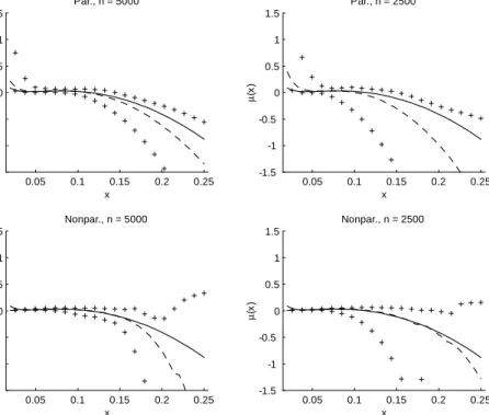
and a restricted version of the model proposed in Aït-Sahalia (1996b),
dXt= 1+ 2Xt+ 3Xt2+ 4Xt 1 dt+
q
1X 2
t dWt: (AS)
The data-generating parameters are chosen to match the estimates obtained when …tting the model by MLE to the Eurodollar interest rate data considered in Aït-Sahalia (1996a,b). The parameter estimates satisfy the -mixing conditions found in Aït-Sahalia (1996b) such that (A.1) holds. We measure time in years and set the time distance to = 1=252, thereby e¤ectively ignoring holidays and weekends, and consider two sample sizes, n= 2500,5000.
For each sample, we estimate the two following semiparametric models when either CKLS or AS is the data generating process respectively: CKLS 1: (x) unknown and 2(x) =
1x 2;
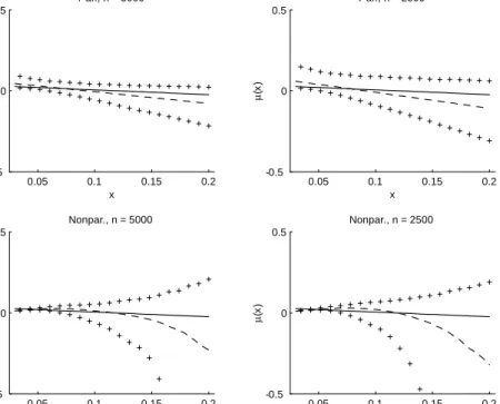
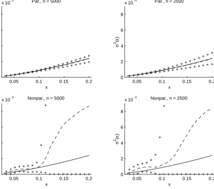
CKLS 2: (x) = 1+ 2x and 2(x) unknown; AS 1: (x) unknown and 2(x) = 1x 2; and AS 2: (x) = 1 + 2x+ 3x2 + 4x 1 and 2(x) unknown. The parameters of the semiparametric models are estimated using the method proposed in Kristensen (2010). Once the parametric component has been estimated, we calculate^ (x)and ^2(x)for models in Class 1 and 2 respectively. We also estimate the fully parametric models (CKLS)-(AS) by MLE which allows us to compare the semiparametric and parametric estimates. In order to evaluate the likelihood in both the parametric and semiparametric case, we employ the simulated likelihood method of Kristensen and Shin (2008). This is implemented by simulating N = 100values for each observation, using the Euler scheme with a step length of = =10 ( (see Kristensen, 2010, for more details)
We …rst investigate the behaviour of the nonparametric estimators for the CKLS model. We consider two sets of data generating parameter values, (i) = (1:8207;2:6217), =