MPRA
Munich Personal RePEc Archive
Equation by equation estimation of the
semi-diagonal BEKK model with
covariates
Le Quyen Thieu
University Pierre and Marie Curie
1 September 2016
Online at
https://mpra.ub.uni-muenchen.de/75582/
Equation by equation estimation of the semi-diagonal
BEKK model with covariates
Le Quyen Thieu,
∗Université Pierre et Marie Curie.
Abstract
This paper provide the asymptotic normality of the Equation by Equation esti-mator for the semi-diagonal BEKK models augmented by the exogenous variables. The results are obtained without assuming that the innovations are independent, which allows investigate dierent additional explanatory variables into the informa-tion set.
Keywords: BEKK-X, Equation by equation estimation, exogenous variables, covariates, semi-diagonal BEKK-X
1 Introduction
Volatility modeling plays an crucial role in the study of nancial mathematics, economics and statistics. Understanding volatilities of nancial asset returns is important in hedg-ing, risk management, and portfolio optimization. The family of GARCH has been widely used to model and forecast volatility (see Bollerslev and Wooldridge (1992) for a com-prehensive review). In particular, multivariate GARCH models are popular for taking into account nancial volatilities co-movements by estimating a conditional covariance
∗Corresponding author: Le Quyen Thieu, Université Pierre et Marie Curie, France. Telephone:
matrix. Recent developments in the estimation of multivariate second moment spec-ications include, among others, the constant conditional correlation (CCC) model of
Bollerslev (1990), the BEKK model of Engle and Kroner (1995), the Factor GARCH model ofEngle and Rothschild (1990), and the Dynamic Conditional Correlation (DCC) model of Engle (2002). One of the challenges in modeling second moments is to ensure the positive deniteness of the resultant covariance matrix without spuriously imposing a temporal pattern in conditional covariances. To cope with this issue, the BEKK model is one of the most exible GARCH models that guarantees the time-varying covariance matrix to be positive denite by construction. However, the conditional covariance ma-trix is only explained by the past returns and volatilities while, in practice, many extra information, under the form of exogenous variables, can help explaining and forecasting nancial volatility. For example, stock or portfolio covariances may be dependent on own nancial characteristics such as liquidity measures, protability measures, or valuation measures like price-to-book or cash-ow-to-book. In addition, overall market forces such as general credit market conditions might impact conditional covariances. It is, there-fore, natural to ask for possible extensions of time series models to accommodate the wealth of information. Engle and Kroner (1995) suggest the BEKK model augmented by exogenous covariates (so-called BEKK-X). However, they only provide the estimation the BEKK model without impact of the covariates. Thieu (2016) presents the variance targeting estimation (VTE) of the BEKK-X model and establishes the Consistency and Asymptotic Normality (CAN) of the VTE. The BEKK-X model is also related to recent literature on GARCH models extended by additional explanatory variables (GARCH-X) with the aim of explaining and forecasting the volatility. Examples of such GARCH-X models include, amongst other, the heavy model of Shephard and Sheppard (2010), the GARCH-X(1,1)ofHan and Kristensen(2014), the Power ARCH(p, q)-X model ofFrancq
and Thieu(2015), the Multivariate Log-GARCH-X model ofFrancq and Sucarrat(2015). Another challenge in modeling a covariance matrix is the "curse of dimensionality", in particular, in the presence of exogenous variables. Indeed, when the dimension of the time series is large, or when the number of covariates is large, the number of parameters can become very large in MGARCH models. The log-likelihood function may therefore contain a numerous number of local maxima, and dierent starting-values may thus lead
to dierent outcomes. A way of reducing this dimensionality curse is via so-called tar-geting which imposes a structure on the model intercept based on sample information. Variance targeting estimation is originally proposed byEngle and Mezrich(1996). Peder-sen and Rahbek(2014) and Thieu (2015) consider this estimation method for the BEKK model and the BEKK-X model, respectively. Despite the potential benets of the VT estimation, it remains some diculties. Enforcing positive deniteness of the conditional covariance matrices the model with targeting implies a set of model constraints that are nonlinear in parameters. This becomes very complicated, except for the scalar case. Moreover, an important question is how much we lose in terms of statistical t in moving from a BEKK/BEKK-X model to a restricted model with fewer parameters to estimate. Finally, in presence of covariates, the curse of dimensionality is still problematic.
In the present paper, I consider an approach that is so-called equation by equation (EbE) estimation to the semi-diagonal BEKK model with presence of the exogenous variables. This statistical method is initially proposed by Engle and Sheppard (2001) and Engle (2002) in the context of DCC models. The EbE method deals very eec-tively with high-dimensional problems and computationally costly log-likelihood. The asymptotic results for the EbE estimator (EbEE) of the volatility parameters, based on Quasi-Maximum Likelihood (QML) are developed in Francq and Zakoïan (2016). In their frame work, they only provide the asymptotic normality of the volatility parameter of the semi-diagonal without covariates. The asymptotic distribution of the estimator of the matrix intercept has not been given. The rst goal of the present paper is to establish the strong consistency and the asymptotic distribution for the EbEE of the individual volatilities parameters of the semi-diagonal BEKK-X model. The second goal is to provide asymptotic results for the estimators of all matrix parameters.
The rest of paper is organized as follows. Section 2 introduces the BEKK model augemented with exogenous variables and presents the EbE method. The consistency and asymptotic behavior of the EbE estimators are investigated in Section 3. Section 4
contains the numerical illustrations. Section 5 concludes. All auxiliary lemmas and mathematical proofs are contained in Section 6.
Some notation and denition throughout the paper: For m, n ∈ N, Im denotes the
denoted by tr(A), the determinant is denoted by det(A) and the spectral radius of A is
denote byρ(A), i.e.,ρ(A)is the maximum among the absolute values of the eigenvalues of A. The operatorvecstacks all columns of a matrix into a column vector,vechdenotes the
operator that stacks only the lower triangular part including the diagonal of a symmetric matrix into a vector, and vech0 is the operator which stacks the sub-diagonal elements
(excluding the diagonal) of a matrix. The (mn × mn) commutation matrix Mmn is
dened such that, for any(m×n)matrix A, Mmnvec(A) = vec(A0). Dm and Lm denote
the duplication matrix and elimination matrix dened such that , for any symmetric
(m×m) matrix A, vec(A) = Dmvech(A) and vech(A) = Lmvec(A). Denote Tm be a
m×m(m+ 1)/2 matrix such that Tmvec(A) = diag(A) for any m×m matrix A. Let
also Pm be a (m(m
−1) 2 ×m
2) matrix such that vech0(A) = P
mvec(A), for any symmetric
(m×m) matrix A. The Kronecker product of A and B is dened by A⊗B = {aijB}.
The Euclidean norm of the matrix, or vector A, is dened as kAk=ptr(A0A), and the
spectral norm is dened askAksp = p
ρ(A0A).
2 The model and EbE estimation
2.1 The model
Let εt = (ε1t,· · · , εmt)0 denote a (m × 1) vector of random variables and let xt =
(x1t,· · · , xrt)0 be a r-dimentional vector of exogenous variables. Assume the existence
of the (m×m)positive denite matrix Ht such that
E(εt|Ft−1) = 0, E(εtε0t|Ft−1) =Ht, (1)
where Ft = σ{εu,x0u;u, u0 ≤ t} implies the information set at time t. Note that Ht is
the conditional covariance of εt given Ft−1 the information set until time t−1.
We consider the following model
εt=H 1/2 t ηt Ht=Ω+Aεt−1ε0t−1A 0 +BHt−1B+Cxt−1x0t−1C 0 (2)
whereA= (ak`)1≤k,`≤m,B=diag(b1,· · · , bm),C = (ck`)1≤k≤m,1≤`≤randΩ= (ωk`)1≤k,`≤m
When there is no covariate (2) is called the semi-diagonal BEKK (see Francq and Zakoïan (2016)). Our model (2) can be so-called the semi-diagonal BEKK-X model.
Throughout of the paper, the following assumptions are made
A1: E(ηt|Ft−1) =0, V ar(ηt|Ft−1) =Im.
A2: (εt,xt) is strictly stationary and ergodic process.
A3: E(kεtk2)<∞ and E(kxtk2)<∞.
Remark 1 In many multivariate GARCH models, it is usual to assume that (ηt) is an
iid white noise vector with zero mean and identity variance matrix. Comte and Lieberman
(2003) and Pedersen and Rahbek (2014) establish the CAN of QMLE and VTE, respec-tively, for the BEKK model under this assumption. Francq and Zakoïan (2016) also provide the CAN of the EbEE for the semi-diagonal BEKK without covariate also under the assumption that the innovation process is iid. However, in presence of the exogenous variables, Assumption A1 is weaker and seems more exible than the iid assumption as several information sets Ft with dierent explanatory variables can be investigated. In
univariate case, Francq and Thieu(2015) study the APARCH-X model under an assump-tion like A1.
Denoting by σ2
kt the k-th diagonal element of Ht, that is the variance of the k-th
component, εkt, of εt conditional on Ft−1
V ar(εkt|Ft−1) =σkt2 .
Dene Dt as the diagonal matrix containing the conditional variances σkt2 , i.e. Dt =
diag(σ1t, . . . , σmt) and let η∗t = D
−1
t εt be the standardized returns. From (1), we have
E(η∗t|Ft−1) = 0 and V ar(η∗t|Ft−1) =D−t1HtD−t1. It follows that the components η
∗
kt of η∗t satisfy, for k = 1, . . . , m,
E(η∗kt|Ft−1) = 0, V ar(ηkt∗|Ft−1) = 1. (3)
The individual volatilities are then parameterized as follows
εkt=σktη∗kt, σ2 kt=ωkk+ m P `=1 ak`ε`,t−1 2 +b2 kσk,t2 −1+ r P s=1 cksxs,t−1 2 . (4)
To ensure the positivity of the volatilities, we assume that ωkk >0. In view of (3), the
process (η∗t)can be called the vector of equation by equation (EbE) innovations of (εt).
Let a0
k = (a0k1, ..., a0km)
0 and c0
k = (c0k1, . . . , c0kr)
0 be, respectively, the k-th row vectors of
the matrices A0 and C0. Then the vector of unknown parameters involved in the k-th
equation (4) can be denoted byθ(0k) = (ω0
kk,a0 0 k,(b0k)2,c0 0 k) 0 ∈ Rd, d=m+r+ 2. It is clear
that an identiability condition must be required such thatσ2
ktis invariant to a change of
sign of the vectors a0k,c0k andb0k. Without lost of generality, we can assume thata0k1 >0, b0 k >0and c0k1 >0, fork = 1, . . . , m. Letθ(k)= (ωkk,a0k, b2k,c 0 k) 0 = (ωkk, ak1, ..., akm, bk, ck1, . . . , ckr)0 be a generic parameter
vector of the parameter space Θ(k) which is an any compact subset of
(0,+∞)2 ×Rm−1×[0,1)×(0,+∞)×
Rr−1.
2.2 Equation-by-equation estimation of parameters
Let ε1, . . . ,εn be observations of a process satifying the semi-diagonal BEKK-X
repre-sentation (2) and x1, . . . ,xn be observations of a process of the explanatory variables.
For all θ(k) ∈Θ(k), we recursively dene σekt2(θ(k)) for t= 1, . . . , n by
e σkt2(θ(k)) = ωkk+ m X `=1 ak`ε`,t−1 !2 +b2keσ2k,t−1(θ(k)) + r X s=1 cksxs,t−1 !2 (5) with the arbitrary initial values eε0,σe0 and x0. Let
e Q(nk)(θ(k)) = 1 n n X t=1 ˜ `kt(θ(k)), `˜kt(θ(k)) = logeσ 2 kt(θ (k)) + ε2kt e σ2 kt(θ (k) ).
The EbE estimator, denoted by θˆ(k)
n , of the true parameter vector θ
(k)
0 is dened as a
measurable solution of the following equation
b θ(nk) = arg min θ(k)∈Θ(k) e Q(nk)(θ(k)). (6) Let θ0 = θ(1)0 0, . . . ,θ(0m)0 0
. Note that θ0 includes the diagonal elements of Ω0 and
all components of the matrices A0,B0 and C0. This parameter vector belongs to the
parameter space Θm = Θ(1) × · · · ×Θ(m), whose generic element is denoted by θ =
θ(1)0, . . . ,θ(m)0
0
. The estimator of θ0 is given by θbn = b θ(1) 0 n , . . . ,θb (m)0 n 0 which is the collection of the equation by equation estimators.
Once the EbEE estimators Abn, Bbn and Cbn of the matrices A0,B0 and C0,
respec-tively, are obtained, the matrix Ω0 can be fully estimated as follows
vech0(Ωbn) = vech0 b Σεn−AbnΣbεnAb 0 n−BbnΣbεnBbn−CbnΣbxnCb 0 n , (7) where Σbεn = 1 n Pn t=1εtε 0 t and Σbxn = 1 n Pn t=1xtx 0
t are the empirical estimators of the
second order moment matrices Σε = E(εtε0t) and Σx = E(xtx0t), respectively. The
estimation of the model (2) is thus nothing else than the estimation of
ϑ0 = (θ00,γ 0 ε0,γ 0 x0) 0 , γε0 =vech(Σε), γx0 =vech(Σx).
Its estimator can be given by ϑbn = (bθ
0 n,γb 0 εn,γb 0 xn) 0, where b γεn = vech(Σbεn) and b γxn = vech(Σbxn).
3 EbE estimation inference
For the consistency of the estimator, the assumptions following will be made A4: θ(0k) ∈Θ(k),Θ(k) is compact, for k= 1, . . . , m.
A5: ρ(A0⊗A0+B0⊗B0)<1 and
Pm
k=1b2k <1, for all θ
(k) ∈
Θ(k).
A6: There exists s >0such that E|εkt|s<∞ and E|xkt|s <∞.
A7: For all `∗ = 1, . . . , m, ε2
`∗t does not belong to the Hilbert space generated by the
linear combinations of the ε`uε`0u's, the xsvxs0v's for u < t, v ≤ t, `, `0 = 1, . . . , m,
s, s0 = 1, . . . , r and the ε`tε`0t for (`, `0)6= (`∗, `∗).
A8: For all s∗ = 1, . . . , r, x2
s∗t does not belong to the Hilbert space generated by the
linear combinations of the the xsvxs0v's for v < t, s, s0 = 1, . . . , r and the xstxs0t for
(s, s0)6= (s∗, s∗).
Remark 2 Assumptions A7 and A8 are identication conditions. For simplicity, let us consider (2) when m= 2, r= 2 and the conditional covariance matrix is given by
Ht=Ω+Aεt−1ε0t−1A
0
+Cxt−1x0t−1C
0
where Ω = ω11 ω12 ω12 ω22
is a symmetric positive denite matrix, A = a11 a12 a21 a22 and C = c11 c12 c21 c22
, with a11 >0, a21 >0, c11 >0 and c21>0. The volatility of the
rst component, ε1t, of εt is thus given by
σ12t =ω11+a11ε21,t−1+2a11a12ε1,t−1ε2,t−1+a12ε22,t−1+c11x21,t−1+2c11c12x1,t−1x2,t−1+c12x22,t−1.
Assumption A7 precludes, for example, that x1,t−1 = ε1,t−1 for which the model is not
identiable.
Similarly, Assumption A8 rules out the existence of linear combination of a nite number of the xs,t−ixs0,t−i that is obviously necessary for the identiability.
Theorem 1 Under A1 - A8, the EbEE of θ(0k) is strongly consistent b
θ(nk) →θ(0k), a.s. as n→ ∞.
The following result is an immediate consequence of Theorem 1.
Corollary 1 Under the assumptions of Theorem1, ϑnb is a strongly consistent estimator
of ϑ0.
Now we turn to the asymptotic distribution of the estimation. We need some addi-tional assumptions.
A9: θ(0k) belongs to the interior of the parameter spaceΘ(k), fork = 1, . . . , m.
A10: Ekηtk4(1+δ) <∞, E||ε
t||4(1+1/δ) <∞and E||xt||4(1+1/δ) <∞ for some δ >0.
A11: The process zt= (x0t,εt0,η0t)0 satises Ekεtk(4+2ν)(1+1/δ) <∞, Ekxtk(4+2ν)(1+1/δ)<
∞andEkηtk(4+2ν)(1+δ)<∞, moreover the strong mixing coecients,α
z(h), of the
process (zt) are such that
∞
X h=0
LetHt,s(ϑ)be such that, for s >0, vec(Ht,s(ϑ)) = s X k=0 (B⊗2)k vec(Ω) +A⊗2vec(εt−k−1ε0t−k−1) +C ⊗2vec(x t−k−1x0t−k−1) ,
where A⊗2 denotes the Kronecker product of a matrix A and itself. Let also S be a
subspace such that for all ϑ ∈Θ, Ht(ϑ)∈ S and for all s >0, Ht,s(ϑ)∈ S.
A12: There exists K >0such that
H 1/2 t (ϑ)−H ∗1/2 t (ϑ) ≤KkHt(ϑ)−H ∗ t(ϑ)k for all Ht(ϑ),H∗t(ϑ)∈ S.
Remark 3 Assumptions A11 and A12 are also required in Thieu (2016) for the BEKK-X model estimated by the variance targeting method.
In order to state the asymptotic normality, we have to introduce the following notations. Let the(d×d)matrices Jks=E(∆kt∆0st), k, s= 1, . . . m, where ∆kt =
1 σ2 kt ∂σ2 kt(θ (k) 0 ) ∂θ(k)
and letJ =diag{J11, . . . ,Jmm}in bloc-matrix notation. Let also∆t=diag(∆1t, . . . ,∆mt), N1 =Lm(Im2 −A⊗02−B⊗02)−1(Im2 −B⊗02) and N2 =Lm(Im2 −A⊗02 −B⊗02)−1C⊗02Dr.
We also dene the following matrices
Σ11= ∞ X h=−∞ cov Υ0tvec(ηtη 0 t),Υ0,t−hvec ηt−hη 0 t−h , (9) Σ22= ∞ X h=−∞
cov vech(xtx0t), vech(xt−hx0t−h) , (10) Σ12= ∞ X h=−∞
cov vech(xtx0t),Υ0,t−hvec ηt−hη
0 t−h , (11) where Υ0t= ∆tTm D−0t1H10/t2 ⊗D−0t1H10/t2 H10/t2⊗H10/t2 . (12)
Theorem 2 Under A1 - A12, as n→ ∞, √ n b θn−θ0 b γεn−γε0 b γxn−γx0 d → N(0,ΓΣΓ0), (13)
where Γ= −J−1 0 0 0 N1 N2 0 0 Ir(r+1)/2 and Σ= Σ11 Σ12 Σ012 Σ22 . (14)
The original parameter vector is denoted by
ξ0 = (vech0(Ω0))0,θ00
0
∈Rm(m−1)/2+md. (15)
The estimator of ξ0 can be given by bξn = b ω0n,bθ 0 n 0 , where ωbn = vech 0( b Ωn) is the estimator of ω0 =vech0(Ω 0).
The strong consistency and the asymptotic distribution of the estimation is given as follows
Theorem 3 If A1 - A8 hold, the estimator bξn of ξ0 is strongly consistent: b
ξn →ξ0 a.s. as n → ∞.
If, in addition, A9 - A12 hold, then
√ n b ωn−ω0 b θn−θ0 d → N(0,ΩΣΩ0), (16) where Ω= Ω1 Ω2 , Ω1 = A∗ B∗ C∗ E∗ X∗ Ψ, Ω2 = Imd 0m(m+1)/2 0r(r+1)/2 , (17) with A∗ =−Pm{Im⊗(A0Σε) + ((A0Σε)⊗Im)Mmm}, B∗ =−Pm{Im⊗(B0Σε) + (B0Σε)⊗Im}, C∗ =−Pm{Im⊗(C0Σx) + ((C0Σx)⊗Im)Mmr}, E∗ =Pm(Im2 −B0⊗B0−A0⊗A0)Dm, X∗ =−Pm(C0⊗C0)Dr.
4 Numerical illustrations
This section presents the results of Monte Carlo simulations studies aimed at examining the performance of the EbEE of the semi-diagonal BEKK-X model and comparing the nite sample properties of the EbEE and VTE.
First, the quality of the EbEE will be evaluated through a Monte Carlo experiment. To keep the computation burden feasible, we focus on the bivariate case, m = 2, but
the results should generalize in an obvious way to higher dimensions. The vector of the exogenous variables isxt = (x1t,x2t)0 = (zt−1,zt−2)0, wherezt−1 and zt−2 are two lagged
values of an APARCH(1,1)
zt=σtet, σt= 0.046 + 0.027z+t−1+ 0.092z
−
t−1+ 0.843σt−1, (18)
where √2et is i.i.d and follows a Student distribution with 4 degrees of freedom. As
discussed in Remark 1, theηt's do not need to be iid with zero mean and identity variance
matrix. In this experiment, theηt's are assumed to follow a bivariate Student distribution
with (4 +|x1,t−1|) degrees of freedom. The BEKK-X parameter are taken as follows
Ω0 = 0.3 0.2 0.2 0.4 ,A0 = 0.15 0.1 0.1 0.2 ,B0 = 0.8 0.0 0.0 0.9 ,C0 = 0.15 0.05 0.1 0.2 . (19) The data series are generated500times forn= 1000andn = 5000observations. For each
data series, (n+ 500)observations ofεt are simulated and then the rst500 observations
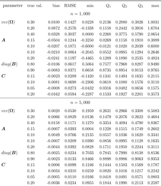
are discarded in each simulation to minimize the eect of the initial values. The results of the simulation study are presented in Table 2. They are in accordance with the consistency of the EbEE, in particular the medians of the estimated parameters are close to the true values. As expected, the accuracy of the estimation increases as the sample size increases from n = 1000to n= 5000.
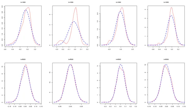
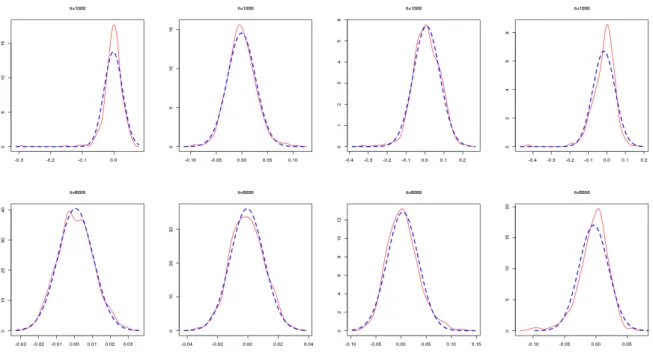
Firgures1,2,3and4show non parametric estimators of the density of the components ofϑbn−ϑ0. As expected, the estimated densities of the estimators over the 500 simulations
are close to a Gaussian density for n suciently large.
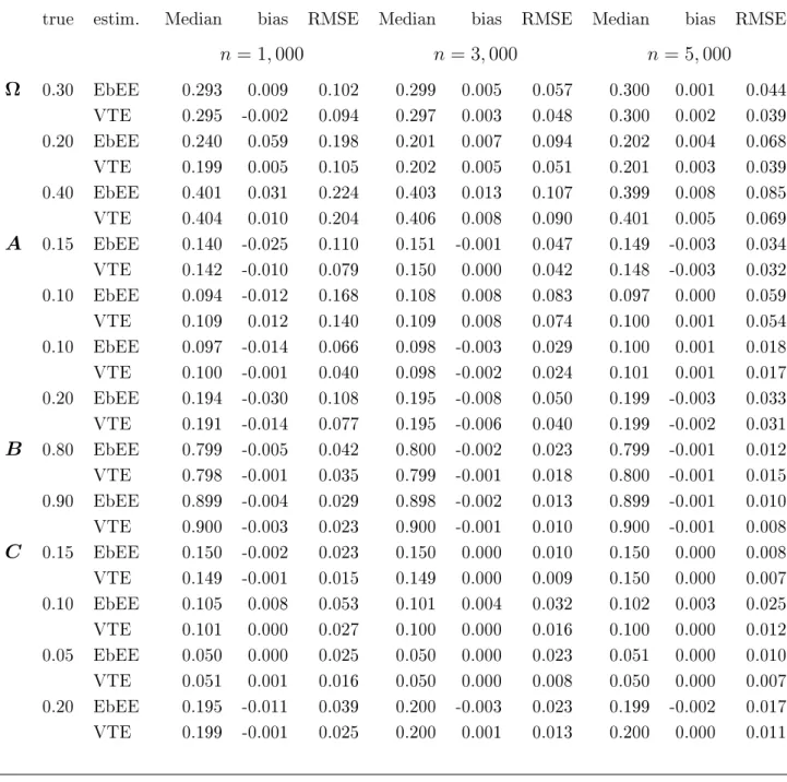
Next, a Monte Carlo experiment is performed with the aim to compare the empirical accuracies of the EbEE and VTE. The true parameter matrices are taken as same as in the previous experiment. ηt are assumed to be independent and normally distributed
N(0,1). Table2summarizes the distributions of the two estimators over500independent
simulations of the model, for the length n = 1000, n = 3000 and n = 5000. From these
Table 1: Sampling distribution of the EbEE of ϑ0 over 500 replications for the BEKK-X(1,1) model
parameter true val. bias RMSE min Q1 Q2 Q3 max
n= 1,000 vec(Ω) 0.30 0.0100 0.1427 0.0228 0.2136 0.2880 0.3826 1.0031 0.20 0.0872 0.2576 -0.1338 0.1158 0.2442 0.3916 1.6704 0.40 0.0328 0.3037 0.0000 0.2268 0.3775 0.5790 2.0654 A 0.15 -0.0504 0.1244 -0.3250 0.0269 0.1158 0.1910 0.3889 0.10 -0.0207 0.1871 -0.6000 -0.0121 0.1020 0.2039 0.6000 0.10 -0.0210 0.0864 -0.2045 0.0552 0.0985 0.1294 0.2646 0.20 -0.0241 0.1197 -0.4465 0.1289 0.1890 0.2535 0.4824 diag(B) 0.80 -0.0106 0.0617 0.5064 0.7577 0.7968 0.8287 0.9490 0.90 -0.0083 0.0371 0.6658 0.8735 0.8954 0.9153 0.9765 C 0.15 -0.0023 0.0289 -0.1420 0.1341 0.1494 0.1635 0.2115 0.10 0.0081 0.0698 -0.2306 0.0618 0.1080 0.1576 0.3110 0.05 -0.0008 0.0273 -0.0432 0.0316 0.0482 0.0656 0.1575 0.20 -0.0162 0.0594 -0.2287 0.1533 0.1927 0.2201 0.3573 n= 5,000 vec(Ω) 0.30 0.0020 0.0530 0.1959 0.2631 0.2966 0.3308 0.5083 0.20 0.0066 0.0829 0.0136 0.1479 0.2076 0.2622 0.4684 0.40 0.0158 0.1171 0.1270 0.3354 0.4094 0.4790 0.8367 A 0.15 -0.0007 0.0393 0.0004 0.1228 0.1515 0.1749 0.2602 0.10 0.0049 0.0766 0.2135 0.0557 0.1036 0.1620 0.3341 0.10 -0.0007 0.0209 0.0390 0.0856 0.0995 0.1128 0.1635 0.20 -0.0044 0.0392 0.0828 0.1711 0.1950 0.2244 0.3111 diag(B) 0.80 -0.0025 0.0234 0.7033 0.7845 0.7990 0.8138 0.8536 0.90 -0.0023 0.0133 0.8466 0.8898 0.8986 0.9063 0.9353 C 0.15 0.0006 0.0099 0.1246 0.1444 0.1503 0.1569 0.1787 0.10 0.0034 0.0310 0.0259 0.0820 0.1016 0.1217 0.2242 0.05 -0.0005 0.0110 0.0166 0.0418 0.0491 0.0571 0.0803 0.20 -0.0036 0.0234 0.0955 0.1844 0.1990 0.2113 0.2597 RMSE is the Root Mean Square Error, Qi,i= 1,3, denote the quartiles.
Figure 1: Kernel density estimator (in full line) of the distribution of the EbEE errors for the estimation of the parameters involved vech(Ω).
Figure 2: Kernel density estimator (in full line) of the distribution of the EbEE errors for the estimation of the parameters involved A.
Figure 3: Kernel density estimator (in full line) of the distribution of the EbEE errors for the estimation of the parameters involved diag(B).
Figure 4: Kernel density estimator (in full line) of the distribution of the EbEE errors for the estimation of the parameters involved C.
and n = 5000. But the dierences are tiny when n is suciently large, for example
n = 3000and n= 5000. Thus, the EbE approach does not seem to create a serious bias
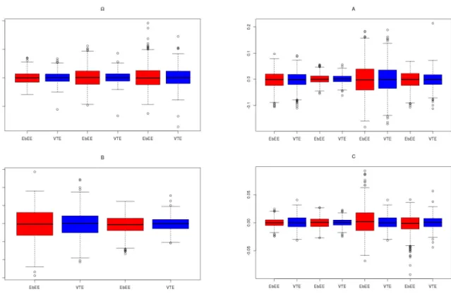
problem in the estimation of the dynamic parameters. Figure 5displays the distribution of the estimation errors for simulations of length n = 5000. The upper-left, upper-right,
bottom-left and bottom-right panels correspond respectively to the estimation errors for the parameters involved in vech(Ω), A,diag(B) and C. The distributions of the EbEE
and VTE are quite similar.
Figure 5: Boxplots of 500 estimation errors for the EbEE and VTE.
5 Conclusion
This paper suggest an eective approach, equation by equation estimation method, for estimation and inference on the semi-diagonal BEKK included the exogenous variables. This approach is recently widely used by researchers and practitioners, consisting in esti-mating separately the individual volatilities parameters in the rst step, and estiesti-mating
Table 2: Sampling distribution of the EbEE and VTE of ϑ0 over 500 replications for the BEKK-X(1,1) model
true estim. Median bias RMSE Median bias RMSE Median bias RMSE
n = 1,000 n = 3,000 n= 5,000 Ω 0.30 EbEE 0.293 0.009 0.102 0.299 0.005 0.057 0.300 0.001 0.044 VTE 0.295 -0.002 0.094 0.297 0.003 0.048 0.300 0.002 0.039 0.20 EbEE 0.240 0.059 0.198 0.201 0.007 0.094 0.202 0.004 0.068 VTE 0.199 0.005 0.105 0.202 0.005 0.051 0.201 0.003 0.039 0.40 EbEE 0.401 0.031 0.224 0.403 0.013 0.107 0.399 0.008 0.085 VTE 0.404 0.010 0.204 0.406 0.008 0.090 0.401 0.005 0.069 A 0.15 EbEE 0.140 -0.025 0.110 0.151 -0.001 0.047 0.149 -0.003 0.034 VTE 0.142 -0.010 0.079 0.150 0.000 0.042 0.148 -0.003 0.032 0.10 EbEE 0.094 -0.012 0.168 0.108 0.008 0.083 0.097 0.000 0.059 VTE 0.109 0.012 0.140 0.109 0.008 0.074 0.100 0.001 0.054 0.10 EbEE 0.097 -0.014 0.066 0.098 -0.003 0.029 0.100 0.001 0.018 VTE 0.100 -0.001 0.040 0.098 -0.002 0.024 0.101 0.001 0.017 0.20 EbEE 0.194 -0.030 0.108 0.195 -0.008 0.050 0.199 -0.003 0.033 VTE 0.191 -0.014 0.077 0.195 -0.006 0.040 0.199 -0.002 0.031 B 0.80 EbEE 0.799 -0.005 0.042 0.800 -0.002 0.023 0.799 -0.001 0.012 VTE 0.798 -0.001 0.035 0.799 -0.001 0.018 0.800 -0.001 0.015 0.90 EbEE 0.899 -0.004 0.029 0.898 -0.002 0.013 0.899 -0.001 0.010 VTE 0.900 -0.003 0.023 0.900 -0.001 0.010 0.900 -0.001 0.008 C 0.15 EbEE 0.150 -0.002 0.023 0.150 0.000 0.010 0.150 0.000 0.008 VTE 0.149 -0.001 0.015 0.149 0.000 0.009 0.150 0.000 0.007 0.10 EbEE 0.105 0.008 0.053 0.101 0.004 0.032 0.102 0.003 0.025 VTE 0.101 0.000 0.027 0.100 0.000 0.016 0.100 0.000 0.012 0.05 EbEE 0.050 0.000 0.025 0.050 0.000 0.023 0.051 0.000 0.010 VTE 0.051 0.001 0.016 0.050 0.000 0.008 0.050 0.000 0.007 0.20 EbEE 0.195 -0.011 0.039 0.200 -0.003 0.023 0.199 -0.002 0.017 VTE 0.199 -0.001 0.025 0.200 0.001 0.013 0.200 0.000 0.011 RMSE is the Root Mean Square Error.
the remaining parameters of the intercept matrix in the second step. The strong consis-tency of the EbEE is showed under the assumptions that are weaker than the ones for the VTE of the same model. Under the mixing-conditions, the asymptotic distribution of the estimators of the parameters is normal. The main motivation for using the EbE method in application is the important gains in computational time and our experiments show that the reduction of computational time compared to the VT estimation can be eective.
6 Proofs
Proof of Theorem 1. Let Q(nk)(θ(k)) = 1 n n X t=1 `kt(θ(k)), `kt(θ(k)) = logσ2kt(θ (k) ) + ε 2 kt σ2 kt(θ (k)).To prove the theorem of the consistency of the EbEE, the following results have to be shown i) lim n→∞ sup θ(k)∈Θ(k) Q (k) n (θ(k))−Qe (k) n (θ(k)) = 0 a.s. ii) σ2 kt(θ (k) 0 ) = σ2kt(θ (k) ) a.s. i θ(0k) =θ(k). iii) E`kt(θ(0k))<∞ and if θ (k)6 =θ(0k) then E`kt(θ0(k))< E`kt(θ(k)).
iv) There exists a neighborhood V(θ(k)) of any θ(k)6=θ(0k) such that
lim inf n→∞ θ∗∈Vinf(θ(k)) e Q(nk)(θ∗)>lim sup n→∞ e Q(nk)(θ(0k)), a.s. The condition Pm k=1b 2
k <1of Assumption A5 and the compactness of Θ
(k) imply that
sup
θ(k)∈Θ(k)
b2k <1. (20)
By a simple recursion, we have
sup θ(k)∈Θ(k) eσ 2 kt(θ (k))−σ2 kt(θ (k)) = sup θ(k)∈Θ(k) (b2k)t eσ 2 k0(θ (k))−σ2 k0(θ (k)) < Kρ t a.s.
where, here and the sequel of the paper, K and ρ denote generic constants whose the
The proofs of i), iii) and i) are very similar to the ones given in Francq and Zakoïan
(2010) for the standard GARCH without covariates and are omitted. Here I only thus show the point ii).
Let L be the back-shift operator, i.e. L(ut) =ut−1. By Assumption A5, the
polyno-mial 1−b2
kL is invertible for any θ
(k) ∈Θ(k). Assume that σ2 kt(θ (k) 0 ) = σkt2 (θ (k)) a.s. We have (1−(b0k)2L)−1 m X `=1 a0k`ε`,t−1 !2 −(1−b2kL)−1 m X `=1 ak`ε`,t−1 !2 + (1−(b0k)2L)−1 r X s=1 c0k`xs,t−1 !2 −(1−b2kL)−1 r X s=1 cksxs,t−1 !2 =(1−b2k)−1ωkk−(1−(b0k) 2)−1ω0 kk a.s. Then ∞ X i=0 m X `,`0=1 a(i``k)0ε`,t−i−1ε`0,t−i−1+ ∞ X j=0 r X s,s0=1 c(jssk)0xs,t−j−1xs0,t−j−1 =c a.s. (21) where a(i``k)0 = (b0k)2ia0k`ak`0 0 −(bk)2iak`ak`0, c(k) jss0 = (b0k)2ic0ksc0ks0 −(bk)2ickscks0 and c= (1− (b0 k)2) −1ω kk −(1−b2k) −1ω0
kk. If b0k 6= bk or there exists `∗ such that a0k`∗ 6= ak`∗ then
ε2`∗,t−1 is a linear combination of the xs,uxs0,u, s, s0 = 1, . . . , r, u < t, the ε`,vε`0,v, `, `0 =
1, . . . , m, v < t−1and theε`,t−1ε`0,t−1,(`, `0)6= (`∗, `∗)which is impossible by Assumption
A7. Thereforeb0k =bk and ak`0 =ak` for all ` = 1, . . . , m and (21) becomes
∞ X j=0 r X s,s0=1 c(jssk)0xs,t−j−1xs0,t−j−1 =c a.s.
Similarly, if there exists s∗ such that c0
ks∗ 6= cks∗, x2
s∗,t−1 is a linear combination of
xu,t−jxu0,t−j, u, u0 = 1, . . . , r, j > 1 and xs,t−1xs0,t−1,(s, s0) 6= (s∗, s∗) which contradicts
Assumption A8. Therefore we have c0
ks=cks for all s= 1, . . . , r. Hence ii) is proved. 2
For the proof the asymptotic distribution in the Theorem 2, we need the following lemmas
such that E sup θ(k)∈V(θ(0k)) 1 σkt2 (θ(k)) ∂σkt2 (θ(k)) ∂θ(k) 4(1+1/δ) <∞, for some δ >0, (22) E sup θ(k)∈V(θ(k) 0 ) 1 σ2 kt(θ (k) ) ∂2σ2 kt(θ (k)) ∂θ(k)∂θ(k)0 2(1+1/δ) <∞, for some δ >0, (23) E ( sup θ(k)∈V(θ(0k)) σkt2(θ(0k)) σ2 kt(θ (k) ) s) <∞, for any s >0. (24) Proof of Lemma 1
Iteratively using the volatility equation in (4), we obtain
σ2kt(θ(k)) = ∞ X j=0 b2kj ( ωkk+ m X `,`0=1 ak`ak`0ε`,t−j−1ε`0,t−j−1+ r X s,s0=1 ckscks0xs,t−j−1xs0,t−j−1 ) . (25) Derive (25) with respect to θ(k), we get
∂σ2 kt(θ (k)) ∂ωkk = ∞ P j=0 b2kj = 1 1−b2 k , ∂σkt2 (θ(k)) ∂ak` = 2 ∞ P j=0 b2kj m P `0=1 ak`0ε`,t−j−1ε`0,t−j−1, ∂σkt2 (θ(k)) ∂b2 k = ∞ P j=1 jb2(kj−1) ( ωkk+ m P `,`0=1 ak`ak`0ε`,t−j−1ε`0,t−j−1+ r P s,s0=1 ckscks0xs,t−j−1xs0,t−j−1 ) , ∂σ2 kt(θ (k) ) ∂cks = 2 ∞ P j=0 b2kj m P s0=1 cks0xs,t−j−1xs0,t−j−1 .
Silmilar expressions hold for the second order derivatives. Noting that
ωkk := inf
θ(k)∈Θ(k)σ
2
kt>0.
Using the moment conditions A10 and (20), we obtain (22) and (23).
The moment condition (24) will be showed even if some components of a0
k orc0k are
zero. Indeed, there exists a neighborhood V(θ(0k)) such that for all θ(k)∈ V(θ(0k))
σ2 kt(θ (k) 0 ) σ2 kt(θ (k) ) ≤K+K ∞ X j=0 (b0 k)2j b2kj m P `=1 a0 k`6=0 ak` √ ωkk ε`,t−j−1 2 1 + m P `=1 a0 k`6=0 ak` √ ωkk ε`,t−j−1 2 + r P s=1 c0 ks6=0 cks √ ωkk xs,t−j−1 2 1 + r P s=1 c0 ks6=0 cks √ ωkk xs,t−j−1 2 .
For allδ >0, there existsV(θ(0k))such thatb0k≤(1 +δ)bk for allθ(k)∈ V(θ
(k)
0 ). It follows
that for all δ >0 and u ∈(0,1), using the inequality z/(1 +z)≤zu for allz ≥0, there
existsV(θ(0k)) such that
sup θ(k)∈V(θ(0k)) σ2 kt(θ (k) 0 ) σ2 kt(θ (k) ) ≤K+K ∞ X j=0 (1 +δ)jρju m X `=1 a0 k`6=0 ε`,t−j−1 2u + r X s=1 c0 ks6=0 xs,t−j−1 2u .
Denote byk.kd the Ld norm, ford≥1, on the space of real random variables. Using the
Minskowski inequality and choosing u such that Ekε1k2us < ∞ and Ekx1k2us <∞ and
choosing, for instance, δ = 1−ρ
u
2ρu and by Assumption A6, we have sup θ(k)∈V(θ(0k)) σ2 kt(θ (k) 0 ) σ2 kt(θ (k) ) s ≤K +K ∞ X j=0 (1 +δ)jρju m X `=1 a0 k`6=0 kε`,t−j−1k22uus+ r X s=1 c0 ks6=0 kxs,t−j−1k22uus <∞. (24) is thus obtained. 2
Lemma 2 Under assumptions of Theorem 2, for all t, we have
i) E sup θ(k)∈V(θ(0k)) ∂2`kt(θ(k)) ∂θ(k)∂θ(k)0
<∞, for some neighborhood V(θ0(k)) of θ(0k).
ii) √1 n n P t=1 ∂2` kt(¯θ (k) n )
∂θ(k)∂θ(k)0 →Jkk, a.s. for any
¯
θn(k) between θˆn(k) and θ(0k).
iii) Jkk is non singular.
Proof of Lemma 2
The derivatives of `kt(θ(k)) is given by
∂`kt(θ(k)) ∂θ(k) = ( 1− ε 2 kt σ2 kt(θ (k)) ) ( 1 σ2 kt(θ (k)) ∂σ2 kt(θ (k)) ∂θ(k) ) (26) and ∂2` kt(θ(k)) ∂θ(k)∂θ(k)0 = ( 1− ε 2 kt σ2 kt(θ (k)) ) ( 1 σ2 kt(θ (k)) ∂2σ2 kt(θ (k)) ∂θ(k)∂θ(k)0 ) + ( 2 ε 2 kt σ2 kt(θ (k) )−1 ) ( 1 σ2 kt(θ (k) ) ∂σ2 kt(θ (k) ) ∂θ(k) ) ( 1 σ2 kt(θ (k) ) ∂σ2 kt(θ (k) ) ∂θ(k)0 ) . (27)
Using the triangle inequality, i) is obtained by showing the existence of the expectations of the two terms in the right-hand side of (27). Let us consider the rst one. We have, by the Holder inequality,
E sup θ(k)∈V(θ(k) 0 ) ( 1− ε 2 kt σ2 kt(θ (k)) ) ( 1 σ2 kt(θ (k)) ∂2σ2 kt(θ (k)) ∂θ(k)∂θ(k)0 ) ≤ 1 +kηkt∗2k2(δ+1) sup θ(k)∈V(θ(0k)) σ2 kt(θ (k) 0 ) σ2 kt(θ (k) ) 2 sup θ(k)∈V(θ(0k)) 1 σ2 kt(θ (k) ) ∂2σ2 kt(θ (k)) ∂θ(k)∂θ(k)0 2(1+1/δ)
which is nite by (23) and (24).The second product in the right-hand side of (27) can be handled similarly using (22).
To prove ii), by Exercise 7.9 in Francq and Zakoïan (2010), it will be sucient to establish that for any >0, there exists a neighborhood V(θ0(k)) of θ(0k) such that
lim n→∞ 1 n n X t=1 sup θ(k)∈V(θ(0k)) ∂2` kt(θ(k)) ∂θ(k)∂θ(k)0 − ∂2` kt(θ (k) 0 ) ∂θ(k)∂θ(k)0 ≤ a.s. (28)
By the ergodic theorem, the limit in the left-hand side is equal to
E sup θ(k)∈V(θ(k) 0 ) ∂2` kt(θ(k)) ∂θ(k)∂θ(k)0 − ∂2` kt(θ (k) 0 ) ∂θ(k)∂θ(k)0
that is nite by i). This expectation tends to zero when the neighborhoodV(θ(0k))shrinks
to singleton {θ(0k)}. The point ii) is thus proved.
We now turn show the invertibility of Jkk. Assume that Jkk is singular. Then there
exists a vector π ∈R2+m+r such thatπ0∂σkt2 (θ
(k) 0 )
∂θ(k) = 0 a.s. It follows that
π1+ 2 m P `=1 a0 k`ε`,t−1 π0 0 εt−1 0(1+r)×1 +π2+mσk,t2 −1(θ (k) 0 ) +2 r P s=1 c0 ksxs,t−1 π0 0(2+m)×1 xt−1 +b02k π0 ∂σ2 k,t−1(θ (k) 0 ) ∂θ(k) = 0, a.s.
Note that the last term in the left-hand side of this equation is equal to zero by the stationarity. We thus have
π1+ 2 m X `,`0=1 a0k`π1+`0ε`,t−1ε`0,t−1+π2+mσ2 k,t−1(θ (k) 0 ) + 2 r X s,s0=1 c0ksπ2+m+s0xs,t−1xs0,t−1 = 0 a.s.
By the similar arguments used to show ii) in the proof of Theorem1, we can conclude that π = 0. 2 Proof of Theorem 2 Since θb (k) n strongly converges to θ (k)
0 which belongs to the interior of the parameter
space Θ(k), the derivative of the criterion Qe
(k) n is equal to zero at bθ (k) n . Let Jkkn(θ(k)) = 1 n Pn t=1 ∂2`kt(θ(k))
∂θ(k)∂θ(k)0. Applying a Taylor expansion for Q
(k)
n at θ(0k) and the mean-value
theorem gives 0 = 1 n n X t=1 `kt(θ (k) 0 ) ∂θ(k) +Jkkn ¯ θ(nk) θb (k) n −θ (k) 0 , (29) where θ¯(k) n is between bθ (k) n and θ (k)
0 . By the points ii) and iii) in Lemma 2 and the
consistency ofθb (k) n , the matrixJkkn ¯ θ(nk)
is a.s. invertible for suciently largen. Hence
multiplying by √n and solving for √n
b θ(nk)−θ(0k) gives √ nbθ (k) n −θ (k) 0 op(1) = −J−kkn1 θ¯(nk)√1 n n X t=1 `kt(θ (k) 0 ) ∂θ(k) . (30) Let `.t(θ) = ∂`1t(θ(1)) ∂θ(1)0 , . . . , ∂`mt(θ(m)) ∂θ(m)0 !0
. Collecting all these Taylor expansions, we have √ nθbn−θ0 op(1) = J−1√1 n n X t=1 . `t(θ0).
Note thatη∗t =D−0t1H10/t2ηt. From (26), we then have . `t(θ0) = −∆tTmvec ηt∗η∗t0 −D−0t1H0tD−0t1 =−∆tTm D−0t1H10/t2 ⊗2 vecηtη0t−Im . Then, we get √ nθbn−θ0 op(1) = −J−1√1 n n X t=1 ∆tTm D−0t1H10/t2 ⊗2 vecηtη0t−Im . (31)
We now introduce the martingale dierence
νt=vec(εtε0t)−vec(H0t) =
H10/t2⊗H10/t2
In the representation ofvec(H0t)obtained from (2), we replacevec(H0t)byvec(εtε0t)−νt. Then, we get vec(εtε0t−E(εtε0t)) = A ⊗2 0 +B ⊗2 0 vec εt−1ε0t−1−E(εt−1ε0t−1) +C⊗02vec xt−1x0t−1−Ext−1x0t−1 + νt−B⊗02νt−1 .
Note that under assumption A5, the matrix Im2 −A⊗02−B⊗02 is inversible. Taking the
average of the two sides of the equality for t = 1, . . . , n gives
b γε,n−γε,0 =Lm(Im2 −A0⊗2 −B⊗02)−1(Im2 −B⊗02) 1 n n X t=1 νt +Lm(Im2 −A⊗02−B⊗02)−1C⊗02Dr b γx,n−γx,0+op(1), a.s. We then have √ nbθn−θ0 √ n(γbεn−γε) √ n(γbxn−γx) op(1) = −J−1 0 0 0 N1 N2 0 0 Ir(r+1)/2 1 √ n Pn t=1Υ0tvec ηtη 0 t−Im Pn t=1vech(xtx0t−E(xtxt)) .
The arguments for establishing the limiting distribution of √1
n Pn t=1Υ0tvec ηtη 0 t−Im Pn t=1vech(xtx0t−E(xtxt))
being very similar to Lemma 6 in Thieu (2016), I just give a sketch of proof. For any
s >0, the k-th individual volatility in (4) can be written σ2
kt =σ2kts+σ2kts, where σ2kts = s X j=0 b2kj ωkk+ m X `=1 ak`ε`,t−j−1 !2 + r X s=1 cksxs,t−j−1 !2 σ2kts = ∞ X j=s+1 b2kj ωkk+ m X `=1 ak`ε`,t−j−1 !2 + r X s=1 cksxs,t−j−1 !2 .
Then we can write Υ0tvec(ηtηt0 −Im) =Yt,s+Y
∗ t,s, where Yt,s= ∆tsTm D−0ts1H10/t,s2⊗D−0ts1H10/t,s2 H10/t,s2 ⊗H10/t,s2 vec(ηtη 0 t−Im),
with D0ts =diag(σ1ts, . . . , σmts) and ∆ts =diag(∆1ts, . . .∆mts), ∆kts = 1
σ2
kts
∂σ2kts(θ(0k))
∂θ(k) ,
for k = 1, . . . , mand Y∗t,s is stationary and centered process satisfying
lim s→∞lim supn→∞ P n−1/2 n X t=1 Y∗t,s > ! = 0.
Under Assumption A11 and using the same argument as in the reference, we have for some ν and δ >0 H01/t,s2 ⊗H01t,s/2vec(ηtη0t−Im) 2+ν <∞.
Note thatD−0t1H0tD−0t1is the conditional correlation matrix ofεt. BecauseD−0t1H0tD−0t1 =
D−0t1H10/t2 D−0t1H10/t2
0
, all the elements of the matrixD−0t1H10/t2 are smaller than one.
It is thus easy to show that all the ones of the matrix D−0t,s1 H10/t,s2⊗D−0t,s1H10/t,s2 are
also smaller than one. Using the Holder inequality, we then have
∆tsTm D−0t,s1H10/t,s2 ⊗D−0t,s1H10/t,s2 vec(ηtη0t−Im) 2+ν ≤ k∆tsk(2+ν)(1+1/δ) Tm D0−t,s1 H10/t,s2⊗D0−t,s1 H10/t,s2vec(ηtη0t−Im) (2+ν)(1+δ) ≤Kk∆tsk(2+ν)(1+1/δ)kvec(ηtη0t−Im)k(2+ν)(1+δ) <∞,
where the last inequality follows from (20) and Assumption A11. It implies thatkYt,sk2+ν <
∞. The process (Yt,s)t, for sxed, is thus strongly mixing under Assumption A11.
Ap-plying the central limit theorem of Herrndorf (1984), we get
1 √ n Pn t=1Υ0tvec ηtη 0 t−Im Pn t=1vech(xtx0t−E(xtxt)) d → N (0,Σ).
The asymptotic distribution of Theorem 2 thus follows from the Slutzky theorem. 2
The proof of Theorem 3
The strong consistency of bξn is obviously obtained.
Now we turn to its asymptotic normality.
Using the elementary relation vec(ABC) = (C0⊗A)vec(B), we have vec(AbnΣbεnAb 0 n−A0Σε0A00) =vec b AnΣbεn(Ab 0 n−A 0 0) +vecAbn(Σbεn−Σε)A00 +vec (Anb −A0)ΣεA00 =nIm⊗(AbnΣbεn) + ((A0Σε)⊗Im)Mmm o vec(Ab 0 n−A 0 0) + (A0⊗Abn)Dmvech(Σbεn−Σε).
Similary, we also get vec(BbnΣbεnBbn−B0ΣεB0) = n Im⊗(BbnΣbεn) + ((B0Σε)⊗Im) o vec(Bbn−B0) + (B0⊗Bbn)Dmvech(Σbεn−Σε) and vec(CbnΣbxnCb 0 n−C0Σx0C00) = n Im⊗(CbnΣbxn) + ((C0Σx)⊗Im)Mmr o vec(Cb 0 n−C 0 0) + (C0⊗Cnb )Drvech(Σbxn−Σx). Let b A∗n =−Pm n Im⊗(AbnΣbεn) + ((A0Σε0)⊗Im)Mmm o , b B∗n =−Pm n Im⊗(BbnΣbεn) + (B0Σε0)⊗Im o , b C∗n =−Pm n Im⊗(CbnΣbxn) + ((C0Σx0)⊗Im)Mmr o , b En∗ =Pm(Im2−B0⊗Bnb −A0⊗Anb )Dm, cX ∗ n =−Pm(C0 ⊗Cnb )Dr. We then have √ n(ωbn−ω0) = Ab ∗ n Bb ∗ n Cb ∗ n Eb ∗ n cX ∗ n √ n b an−a0 b bn−b0 b cn−c0 b γεn−γε0 b γxn−γx0 , (32) where abn = vec(Ab 0
n), bbn = vec(Bbn) and bcn = vec(Cb
0
n) are the estimators of a0 =
vec(A00), b0 =vec(B0) and c0 =vec(C
0
0)respectively. Note that
b an−a0 b bn−b0 b cn−c0 b γεn−γε0 b γxn−γx0 =Ψ b θn−θ0 b γεn−γε0 b γxn−γx0 , (33)
whereΨis ad1×d2 matrix,d1 = 2m2+mr+m(m2+1)+r(r2+1) andd2 =md+m(m2+1)+r(r2+1),
given by, fork = 1, . . . , m,
Ψ[(k−1)m+ 1 :km,(k−1)(m+r+ 2) + 2 : (k−1)(m+r+ 2) +m+ 1] =Im, Ψ[m2+ (k−1)m+k, k(m+ 2) + (k−1)r] = 1, Ψ[2m2+ (k−1)r+ 1 :m2+m+kr, k(m+ 2) + (k−1)r+ 1 :k(m+r+ 2)] =Ir, Ψ[2m2+mr+ 1 :d1, md+ 1 :d2] =Im(m+1) 2 + r(r+1) 2
and the others entries are zero. We then have
√ n b ωn−ω0 b θn−θ0 =Ωbn √ n b θn−θ0 b γεn−γε0 b γxn−γx0 , (34) where Ωbn = b Ω1n Ω2 with Ωb1n = b A∗n Bb ∗ n Cb ∗ n Eb ∗ n cX ∗ n Ψ. Note that Ωbn is
strongly consistent estimator of Ω. By applying the Slutzky theorem, the asymptotic
normality in Theorem 3is thus obtained. 2
References
Bollerslev, T. (1990) Modelling the coherence in short-run nominal exchange rates: a multivariate generalized ARCH model. The review of economics and statistics 495505.
Bollerslev, T. and J.M. Wooldridge (1992) Quasi-maximum likelihood estimation and inference in dynamic models with time-varying covariances. Econometric re-views 11, 143172.
Boussama, F., F. Fuchs and R. Stelzer (2011) Stationarity and geometric ergodic-ity of BEKK multivariate GARCH models.Stochastic Processes and their Applica-tions 121, 23312360.
Comte, F. and O. Lieberman (2003) Asymptotic theory for multivariate GARCH processes. Journal of Multivariate Analysis 84, 6184.
Engle, R.F., V.K. Ng and K.F. Kroner (1990) Asset pricing with a factor-ARCH covariance structure: Empirical estimates for treasury bills. Journal of Economet-rics 45, 213237.
Engle, R.F. and K.F. Kroner (1995) Multivariate simultaneous generalized ARCH. Econometric theory 11, 122150.
Engle, R.F. and Sheppar, K. (2001) Theoretical and empirical properties of dynamic conditional correlation multivariate GARCH. National Bureau of Economic Re-search.
Engle, R.F. (2002) Dynamic conditional correlation: A simple class of multivariate gen-eralized autoregressive conditional heteroskedasticity models. Journal of Business and Economic Statistics 20, 339-350.
Engle, R. (2009) Anticipating correlations: a new paradigm for risk management. Prince-ton University Press.
Francq, C. and J-M. Zakoïan (1998) Estimating linear representations of nonlinear processes.Journal of Statistical Planning and Inference 68, 145165.
Francq, C. and J-M. Zakoïan (2000) Covariance matrix estimation for estimators of mixing weak ARMA models.Journal of Statistical Planning and Inference 83, 369 394.
Francq, C. and J-M. Zakoïan (2010) GARCH Models: Structure, Statistical Infer-ence and Financial Applications. John Wiley.
Francq, C. and Thieu, L.Q. (2015) Qml inference for volatility models with covari-ates. University Library of Munich, Germany, No. 63198.
Francq, C. and G. Sucarrat (2016) Equation-by-Equation Estimation of a Multivari-ate Log-GARCH-X Model of Financial Returns. Journal of the Royal Statistical Society: Series B 78, 613635,http://onlinelibrary.wiley.com/doi/10.1111/ rssb.12126/epdf
Hafner, C.M. and A. Preminger (2009) On asymptotic theory for multivariate GARCH models.Journal of Multivariate Analysis 100, 20442054.
Han, H. and D. Kristensen (2014) Asymptotic Theory for the QMLE in GARCH-X Models With Stationary and Nonstationary Covariates. Journal of Business & Economic Statistics 32, 416429.
Herrndorf, N. (1984) A functional central limit theorem for weakly dependent se-quences of random variables. The Annals of Probability, 141153.
Pedersen, R.S. and A. Rahbek (2014) Multivariate variance targeting in the BEKK-GARCH model. The Econometrics Journal 17, 2455.
Phillips, P.C.B., Y. Sun and S. Jin (2003) Consistent HAC estimation and robust regression testing using sharp origin kernels with no truncation. Discussion paper, Yale University.
Shephard, N. and Sheppard, K. (2010) Realizing the future: forecasting with high frequency based volatility (HEAVY) models. Journal of Applied Econometrics 25, 197231.
Silvennoinen, A. and T. Teräsvirta (2009) Modeling multivariate autoregressive con-ditional heteroskedasticity with the double smooth transition concon-ditional correlation GARCH model. Journal of Financial Econometrics 7, 373411.