A Hardware Runtime for Task-based
Programming Models
Xubin Tan, Jaume Bosch, Carlos ´
Alvarez, Daniel Jim ´enez-Gonz ´alez, Eduard Ayguad ´e,
and Mateo Valero,
Fellow, IEEE
Abstract—Task-based programming models such as OpenMP 5.0 and OmpSs are simple to use and powerful enough to exploit task parallelism of applications over multicore, manycore and heterogeneous systems. However, their software-only runtimes introduce relevant overhead when targeting fine-grained tasks, resulting in performance losses. To overcome this drawback, we present a hardware runtime Picos++ that accelerates critical runtime functions such as task dependence analysis, nested task support, and heterogeneous task scheduling. As a proof-of-concept, the Picos++ hardware runtime has been integrated with a compiler
infrastructure that supports parallel task-based programming models. A FPGA SoC running Linux OS has been used to implement the hardware accelerated part of Picos++, integrated with a heterogeneous system composed of 4 symmetric multiprocessor (SMP) cores and several hardware functional accelerators (HwAccs) for task execution. Results show significant improvements on energy and performance compared to state-of-the-art parallel software-only runtimes. With Picos++, applications can achieve up to 7.6x speedup and save up to 90% of energy, when using 4 threads and up to 4 HwAccs, and even reach a speedup of 16x over the software alternative when using 12 HwAccs and small tasks.
Index Terms—Fine-grained parallelism; Task-dependence analysis; Nested tasks; Heterogeneous task scheduling; Energy saving; FPGA; Task-based programming models;
F
1
I
NTRODUCTIONP
ARALLEL computing has become an ubiquitousprin-ciple to gain performance on multicore and many-core platforms. However, it exposes significant challenges, such as detecting parallel regions, distributing tasks/works evenly and synchronizing them. Furthermore, current pro-cessor architectures evolve towards more heterogeneity which only aggravates the aforementioned difficulties. Task-based programming models are quickly evolving to target these challenges. Significant examples are OpenMP 5.0 [1], OmpSs [2], etc. Using these programming models, an ap-plication can be expressed as a collection of tasks with dependences, whose execution orders and potential data movements are enforced through dynamically constructing their task dependency graph (TDG) in runtime. Although with moderate size tasks, those programming models are able to exploit high levels of task parallelism with their de-fault software-only runtimes, with fine-grained tasks, they suffer different degrees of performance degradation due to the runtime overhead and thread contention [3], [4], [5].
A straightforward way to overcome this deficiency and enable a finer task parallelism is to improve the overall run-time by accelerating its most critical functions in hardware. For homogeneous multicores, task dependence analysis is the most critical function [5], [6], [7]. For heterogeneous architectures, the task scheduling cost is also very high due to the load balance challenge caused by the execu-tion time difference, the necessary data movements and synchronization between different memories [8], [9], [10]. Previous works of hardware task dependence management • All authors are with the Barcelona Supercomputing Center (BSC) and
Universitat Polit`ecnica de Catalunya (UPC).
E-mail: [email protected],{calvarez, djimenez}@ac.upc.edu
have showed great scalability and performance improve-ment over their software-only alternatives [4], [11], [12], [13]. However, firstly these works did not support nested tasks, that is, tasks that have been created by another task; secondly they did not support task scheduling to different hardware in heterogeneous systems; finally they have not been evaluated in a real system integrated as a hardware support within a programming model runtime. The most comprehensive analysis of a hardware task dependence manager [14] up to the moment was done targeting a small system with only two cores presenting good performance results but with a very limited scope.
In this paper we make a thorough analysis of Picos++, a general purpose hardware for task dependence manage-ment, nested task support and heterogeneous task schedul-ing for task-based programmschedul-ing models. The main contri-butions of this paper are as follows:
• A new heterogeneous task scheduling support. For the first time a hardware task scheduler is able to schedule tasks to different hardware execution units (SMPs and hardware accelerators).
• A novel hardware/software co-design for support-ing nested tasks. The original version developed for SMP only systems has been extended to pre-vent deadlocks when the heterogeneous hardware resources are fully used.
• Picos++ implementation fully integrated with a task-based programming model in a heterogeneous FPGA system running Linux OS and being able to execute problems concurrently in both FPGA and SMP.
• Detailed scalability and energy consumption stud-ies during real executions of applications
compar-Listing 1: multisort with OpenMP directives
1 void m u l t i s o r t ( s i z e t n , T data [ n ] , T tmp [ n ] ) {
2 i n t i = n/4L ; i n t j = n/2L ;
3 i f ( n<CUTOFF) {s e q u e n t i a l s o r t ( . . . ) ;} e l s e {
4 #pragma omp t a s k depend ( i n o u t : data [ 0 ] , tmp [ 0 ] )
5 m u l t i s o r t( i , &data [ 0 ] , &tmp [ 0 ] ) ;
6 #pragma omp t a s k depend ( i n o u t : data [ i ] , tmp [ i ] )
7 m u l t i s o r t( i , &data [ i ] , &tmp [ i ] ) ;
8 #pragma omp t a s k depend ( i n o u t : data [ j ] , tmp [ j ] )
9 m u l t i s o r t( i , &data [ j ] , &tmp [ j ] ) ;
10 #pragma omp t a s k depend ( i n o u t : data [ 3 L∗i ] , tmp [ 3 L∗i ] )
11 m u l t i s o r t( i , &data [ 3 L∗i ] , &tmp [ 3 L∗i ] ) ; 12
13 #pragma omp t a s k depend ( i n : data [ 0 ] , data [ i ] ) \
14 depend ( out : tmp [ 0 ] )
15 merge( i , &data [ 0 ] , &data [ i ] , &tmp [ 0 ] ) ;
16 #pragma omp t a s k depend ( i n : data [ j ] , data [ 3 L∗i ] ) \
17 depend ( out : tmp [ j ] )
18 merge( i , &data [ j ] , &data [ 3 L∗i ] , &tmp [ j ] ) ;
19 #pragma omp t a s k depend ( i n : tmp [ 0 ] , tmp [ j ] ) \
20 depend ( out : data [ 0 ] )
21 merge( j , &tmp [ 0 ] , &tmp [ j ] , &data [ 0 ] ) ;
22 #pragma omp t a s k w a i t }}
ing both Picos++ and software-only runtime sys-tems, where tasks are executed in both threads and HwAccs. For the first time the real executions is ex-tended to up to 15 execution units, providing insight of the impact of the hardware runtime with more hardware devices in the system.
• Execution trace support for application and Picos++ analysis.
The paper is organized as follows: Section 2 describes the background and previous work. Section 3 presents the Picos++ system. In Section 4, the experimental setup and benchmarks are described. Section 5 presents detailed stud-ies of the impact of Picos++ on performance and energy consumption. Finally, in Sections 6 and 7 we discuss related work and conclude this paper.
2
B
ACKGROUND2.1 Task-based Programming Model
OpenMP provides a powerful way of annotating sequential programs with directives to exploit task parallelism. For example in C/C++ language: #pragma omp task depend(in: ...) depend(out: ...) depend(inout: ...) is used to specify a task with the direction of its data dependences (scalars or arrays). Implicit synchronization between tasks is ensured by the task dependence analysis in runtime. Explicit synchronization is managed by using #pragma omp taskwait, which makes a thread wait until all its child tasks finish before it can resume the code execution.
An example of multisortsource code with OpenMP annotations is shown in Listing 1. Each multisort task in-stance can create four child multisort tasks and three child merge tasks as shown in lines 4-21. When the compiler finds a task annotation in the program it outlines the next statement and introduces a runtime system call to create a task (represented as a Task Descriptor). At execution time, the runtime system manages task creation, computes TDG, and schedules tasks when all their dependences are ready. Thetaskwaitpragma at line 22 will wait for all the child tasks to finish.
Listing 2: Matmul block functions with OmpSs annotation
1 #pragma omp t a r g e t d e v i c e ( fpga ) copy deps
2 onto ( 0 ) num instances ( 4 )
3 #pragma omp t a s k i n o u t ( [ bs ]C) i n ( [ bs ]A, [ bs ] B ) 4 void matmulBlock( T (∗A) [ bs ] , T (∗B ) [ bs ] , T (∗C ) [ bs ] ){
5 unsigned i n t i , j , k ; 6 7 #pragma HLS a r r a y p a r t i t i o n v a r i a b l e =A b l o c k f a c t o r =bs /2 8 #pragma HLS a r r a y p a r t i t i o n v a r i a b l e =B b l o c k f a c t o r =bs /2 9 f o r ( i = 0 ; i < bs ; i ++) { 10 f o r ( j = 0 ; j < bs ; j ++) { 11 #pragma HLS p i p e l i n e I I =1 12 T sum = 0 ; 13 f o r ( k = 0 ; k< bs ; k++) { 14 sum += A[ i ] [ k ] ∗ B [ k ] [ j ] ; } 15 C[ i ] [ j ] += sum ; }}} 16
17 #pragma omp t a r g e t d e v i c e ( smp ) no copy deps
18 implements (matmulBlock)
19 #pragma omp t a s k i n ( [ bs ]A, [ bs ] B ) i n o u t ( [ bs ]C)
20 void matmulBlockSmp( T (∗A) [ bs ] , T (∗B ) [ bs ] , T (∗C ) [ bs ] ){
21 T c o n s t alpha = 1 . 0 ; T c o n s t b e t a = 1 . 0 ;
22 cblas gemm ( CblasRowMajor , CblasNoTrans , CblasNoTrans ,
23 bs , b s i z e , bs , alpha , a , bs , b , bs , beta , c , bs ) ;
24 }
2.1.1 Nested tasks
The aforementioned child tasks are also named nested tasks in the OpenMP standard. They are supported to improve the programmability and nested parallelism. For instance, a nested task can be found in recursive code where the recursive function is a task that can be further decomposed (like in Multisort), or even when using tasks to call libraries with embedded tasks. Therefore, nested task support is a necessary feature of any task manager that wants to execute general-purpose code. Besides the fact that a parent task has to wait for all its child tasks, there are two more definitions that are important to consider: 1) A “child task” can only have a subset of its parent task’s dependences. 2) The dependences of a “child task” only affect its sibling tasks (“child tasks of the same parent”).
2.1.2 Heterogeneous Task Scheduling
The OmpSs programming model is developed as a fore-runner for the OpenMP standard. In this work we will use it as an example for heterogeneous task scheduling. Listing 2 shows an example of OmpSs application with two instances of Matmul block functions that can be executed in either HwAccs in FPGA or in SMP threads. For example, the matmulBlock function in line 4 is annotated with both task and target device pragmas. The task pragma indicates the data dependences. The target device indicates that this task is going to be executed in the FPGA. At compile time, 4 instances of type 0 HwAcc for this function are created as indicated byonto(0) num instances(4)clause. In addition,
the copy deps specifies to copy the task dependence data
from the host memory to the HwAccs (for input data) and from the HwAccs to the memory (for output data). The source-to-source Mercurium compiler generates the SMP code with the runtime (Nanos++) calls, task function code for SMP tasks, and the HwAccs for FPGA tasks [15]. Gcc compiler generates the binary code of the SMP, and the Xilinx tools Vivado and Vivado HLS, generate the bitstream of the FPGA.
2.2 Picos Overview
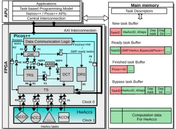
The Picos hardware design [13] started with the aim to accelerate task dependence management for task-based pro-gramming models to exploit fine-grained task parallelism. From the software point of view, it can be seen as a blackbox that (1) reads new tasks and dependences from memory at task creation time; (2) writes ready-to-execute tasks in memory for the worker threads and (3) processes finished tasks.
The first hardware prototype of Picos [4] has a similar architecture to Picos++, shown in Figure 1. Picos is com-posed of five main components.Gateway (GW)fetches new and finished tasks from outside, and dispatches them to Task Reserve Station (TRS) and Dependence Chain Tracker (DCT).TRSis the major task management unit. It stores in-flight tasks, tracks the readiness of new tasks and manages the deletion of finished tasks. It includes a Task Memory (TM) with 256 entries for up to 256 in-flight tasks, not shown in the figure. Each entry stores the task identification (TaskID), the number of dependences per task (#Deps), the position in the DCT where each dependence is saved, and a reference to the next task consumer of each dependence.
DCTis the major dependence management unit. It manages task dependences through one Dependence Memory (DM) and one Version Memory (VM). DM stores the memory addresses of dependences as tags and performs address match for each new dependence to these arrived earlier, to track data dependences. VM keeps the last consumer and the chain of producers of all the references to the same dependence address (called versions).Arbiter (ARB)
manages the communication between TRS and DCT. Task Scheduler (TS)stores all ready tasks and schedules them to idle workers. Each pair of components are connected with FIFOs to ensure asynchronous communications.
Picos uses synchronous communication [4] between soft-ware and hardsoft-ware. In fact, due to the communication mechanism the overall system performance is burdened. Threads are in charge of program- ming the DMA for each data movement (new, ready, finished task) between main memory and Picos. Although simple, this method is costly due to the frequent and small data exchanges in the system.
2.2.1 Hardware task scheduling applicability
Although Picos and Picos++ (as will be explained) have been implemented in a system composed of (few) ARM cores and an FPGA, this implementation aims to be only a proof-of-concept of its usability and capabilities. Picos and Picos++ are designed to work in a different scenario from the one presented. Such scenario is a multicore system of any type of SMP processors (i.e. ARM, Risc-V, Intel, IBM processors, etc.), where Picos++ would be implemented as an ASIC connected to all the cores. In such a system, Picos++ will run at the same frecuency as the cores and manage even more fine grained tasks (as the communication will be faster that in the current implementation). Such system is expected to obtain even higher benefits from hardware task scheduling than the ones obtained in the current paper. If the system is in addition composed of some heterogeneous components (such different SMP cores, FPGAs or GPUs or any other type) Picos++ ASIC will also take care of
S Applications Task-based Programming Model
Nanos++ / Picos++ APIs Task Descriptors
Finished task Buffer Ready task Buffer
New task Buffer
GW
TRS DCT
TS ARB
Main memory
Data Communication Logic
A P U F P G A
HwAccID, #Deps AddrDep DepDir
TaskID (SMP,HwAcc,Bypass)&Picos++ID
Picos++ID
Bypass task Buffer
ACC1 ... ACC0 Clock 0 Clock 1 Computation data For HwAccs DRS ACCN Central Interconnection AXI Interconnection Bypass tasks Finished HW / SMP ready tasks ...
HwAccID, #DepsAddrDep DepDir...
... ... Picos++ TaskID TaskID N2 N1 F1 N3 N4 N5/F4 N6 F2 F3 N5 F5 F6 / R2 R1’ R1 R3 R4 N5/F4 HwAccs HwAcc tasks
Fig. 1: Picos++ system organization
this components. In current environments, the SMP threads are the ones in charge of managing the accelerators and this work also adds overheads that Picos++ ASIC would mitigate.
The same could be said about the programming model used. Although in this paper we target OmpSs as a pro-gramming model that already has good support for FPGA task execution, any task based programming model would benefit from Picos++. The API of Picos++ for receiving a task with dependences, releasing ready tasks and receiving notitifications of finished tasks is general enough to be adapted to other task-based programming models runtimes (e.g. OpenMP runtimes) and even to other programming models. In this sense, the aim of this work is to prove that the task scheduler is one the next components that should be moved from software to hardware in future processors.
3
P
ICOS++ S
YSTEMPicos++ is an evolution of the previous design with sev-eral important new features introduced to support nested tasks, tasks with unlimited number of dependences and heterogeneous task scheduling. The main new components in Picos++ not included in the previous Picos design showed in figure 1 are: the Bypass task buffer stored in main memory for communication, the Dependence Reserve station (DRS) module in Picos++, the TS communication with the hardware accelerators (HwAccs) and the HwAccs themselves. In addition to those, the modifications also include a new hardware-software asynchronous communi-cation scheme [14] and different GW, DCT and TS behaviors, including a new DCT memory as described in section 3.2.
Figure 1 shows the sequence of new (labeled N#) and finished task (labeled F#) processing. The ready task pro-cessing (labeled R#) will be introduced later.When a new task arrives, GW reads the task and its dependences (N1) and requests a free TM entry from TRS (N2). Afterwards, it distributes the task to TRS (N3) and its dependences to DCT (N4). TRS saves the task information including TaskID and#Depsin the corresponding TM entry. DCT performs address match of each dependence to those arrived earlier. If there is no match, DCT notifies TRS that this dependence is ready (N5). Otherwise, there is a possible producer or consumer match, DCT saves the producer match and only
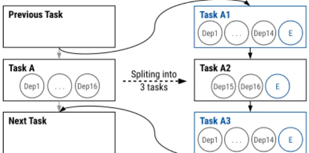
Task A Previous Task Next Task Task A2 Task A1 Task A3 Spliting into 3 tasks Dep1 . . . Dep16 Dep1 . . . Dep14 E Dep1 . . . Dep14 E Dep15 Dep16 E
Fig. 2: Process for managing tasks with more than 15 depen-dences
notifies TRS of the consumer match (N5). By doing this, for all the producer-consumer chain (aka. true-date dependence chains), the producer is saved in DCT while the consumers are saved in TRS. TRS processes all these notifications. For each ready one, TRS checks if all the dependences of this task are resolved; if so, TRS marks it ready and schedules it either to an idle thread or HwAcc (N6) meanwhile TRS forwards a ready message to the next consumer task (if it exists) dependent on this ready dependence (also N5). Otherwise TRS saves this possible consumer match.When a finished task arrives, GW reads (F1) and forwards it to TRS (F2). TRS checks the corresponding TM entry for all the dependences and sends finished notification of them to DCT (F3). DCT checks DM and VM for each finished dependence to either delete its instances or send ready notifications to TRS to wake up the dependences that were previously not ready (F4).
Figure 1 also shows the Picos++ system implementation. It mainly consists of the application processing unit (APU) with SMP inside, a FPGA and a shared main memory. Picos++ and HwAccs are inside the FPGA, using clock domains 0 and 1 respectively. All the data exchange between these two clock domains are dealt with either asychronous FIFOs or clock-crossing (standard method to pass multibits or 1-bit data safely from one clock domain to another).
There are two sets of communications: first is for new, ready, finished and bypass tasks, where Picos++ and APU share them in the main memory; second is the computation data required by the HwAccs. Each HwAcc used is capable of reading input data from the main memory, does com-putation and then writes back results to the main memory, without help from the SMP threads inside APU.
3.1 Hardware/Software Synchronization
For the task communication between SMP threads and Picos++ in FPGA, there are four circular buffers, one for each type of tasks shown in Figure 1. Each buffer can store up to N units representing N tasks. At the beginning of the application execution, the software side of the runtime starts Picos++ and allocates those buffers in main memory. Afterwards, it sends the buffer addresses and lengths to Picos++. When the application finishes, it deallocates the buffers and stops Picos++ [14].
New task buffer stores new task information required
by Picos++. Each new task entry consists of: TaskID (8
bytes), HwAccID (2 bytes), #Dependences (2 bytes), and for
each dependence, the dependence memory address (8 bytes)
and direction (4 bytes). HwAccID identifies which are the
hardware devices where a particular task can be executed (currently, up to 16 different types).
The current hardware implementation supports a max-imum of 15 dependences per task. In the case of more dependences, as this is known at compile time, the task can be splitted into an artificial chain of tasks with at most 15 dependences each. Figure 2 shows how an original task A with 16 dependences is split into three tasks A1, A2 and A3 that have 15 or less dependences per task and maintains the correct execution order. Task A1 will be created with 14 of the original dependences and an Extra (E) helper dependence with inout type. A1 will be a empty task that has no computation. Task A2 will have the remaining 15th and 16th original dependences and the same Extra (E) helper dependence with inout type. It will inherit all the computation from the original Task A. This way through the inout dependence chain, the original code will be executed only after all the original dependences are ready. Finally, another empty helper task A3 will do the same function as task A1. This last task will ensure that any task that depends on any of the 16 original dependences is executed in the correct order. This simple mechanism can be replicated for any number of dependences using more helper tasks. In fact, it allows Picos++ to process tasks with more dependences than fit in its internal memories (as the helper tasks dont need to be processed as a single unit) and maintains the parallel processing in a nested task environment.
Ready task buffer holds not only the ready-to-execute SMP tasks, but also messages that signal the software part of the runtime that a HwAcc has finished executing a ready task. Each unit includes TaskID (8 bytes), (SMP, HwAccs,
Bypass) (3 bits) and Picos++ID (14 bits). For each SMP task
(identified by the SMP bit), the software runtime schedules it to execute in threads; for each finished executing HW task (identified by the HwAcc or Bypass bit), the software run-time deletes the corresponding task descriptor in memory.
Finished task bufferstores the information(Picos++ID)
of finished tasks from threads, to send it back into Picos++ for TDG update. Note that this is only for tasks scheduled to execute in threads. For tasks scheduled to execute in the HwAccs, they are directly sent to HwAccs and retrieved back through separate FIFO queues inside the FPGA. There-fore, those finished tasks would not appear in this buffer.
Bypass task buffer stores bypass tasks, with the same format as the new task buffer. The bypass tasks are already ready to execute. This concept is introduced to tackle two new situations raised by HwAccs. The first one is to handle applications that want to accelerate part of the code using the HwAccs without Picos++ task dependence manager. They need a direct communication mechanism from the APU to the FPGA that bypasses the dependence manager and directly executes in HwAccs. The second situation appears in applications with nested tasks. When all the Pi-cos++ internal task dependence management resources are used up, and this channel allows us to continue executing tasks in HwAccs.
In the case of new, finished and bypass task buffers, SMP threads write to these buffers while Picos++ hardware reads them while in the case of the ready task buffer, the communication works in the opposite direction. For all the buffers, entry fields have valid bits to inform the Picos++
multisort 1.2 multisort 1.3 multisort1.4 merge 1.5 merge1.6 merge 1.7 multisort
2.1 multisort2.2 multisort2.3 multisort2.4 merge 2.5 merge 2.6 merge 2.7 multisort 1.1
Fig. 3: Multisort with nested task dependences hardware and software part that those entries are valid or not, and also the type of tasks.
The data communication between software and Picos++ hardware is important for the final system performance. Picos++ implements a buffered and asynchronous com-munication which requires small support from threads. It decouples the data communication between software and hardware, ensuring an efficient small data exchange suitable for our user case. As a result, Picos++ obtains a high overall system performance [14].
3.2 Nested Task Support
To support nested tasks, we add a new field parentID for each new task in the task buffer. This parentID together with taskID allow the dependences of non-sibling tasks to be maintained in separate TDGs inside Picos++.
Nonetheless, this is not enough to avoid corner cases that can lead to a whole system deadlock. Those corner cases derive from the fact that hardware task managers, opposed to the software ones, have a limited amount of memory. Thus, it is possible for them to read a task and get their internal memory full in the middle of processing task dependences. Without nested tasks, this is not a prob-lem because previous processed tasks go to execution and eventually they finish and free out resources that will allow the hardware to proceed with the stalled tasks.
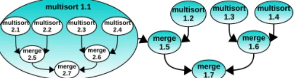
For nested tasks with dependences, the situation is much more complicated. To simplify and explain a possible dead-lock scenario, assume that Picos++ has memory capacity for only 7 tasks. Figure 3 shows the TDG of the Multisort application when two levels of nested tasks have been reached. Tasks in level i are labeled i.X, where X is the number of the sibling task order creation. While all tasks in level 1 are shown, only child tasks of multisort 1.1 are shown for the second level. In this case, the first level tasks would quickly fill the Picos++ hardware manager when the executing multisort 1.1 tries to create new tasks. In partic-ular, multisort 1.1 will create the first child task multisort 2.1, that will get stuck due to a full memory problem. As a parent task multisort 1.1 has to wait until all its child tasks end (and they will not end), it cannot finish and all the following multisort (which can create similar child tasks) and merge1.Xtasks, already inside the hardware manager, can not proceed (and free memory for more tasks), so the system goes into a deadlock.
3.2.1 Deadlock Free Hardware/Software Co-design
In order to support nested tasks without deadlocks, we introduce a hardware/software co-design in Picos++.
Atomic task processingis the hardware solution which offers the first step to avoid deadlocks by reading and processing tasks atomically. Once a task is read all its dependences should be processed (i.e. integrated in the
TDG). Using a non-atomic task processing would allow the GW to read new tasks without considering the free spaces in all the internal memories (TM, DM and VM) until the FIFOs connecting them are full. Without nested tasks, this method ensures efficient inter-component communication. However, it leads to deadlocks easily with nested tasks. For instance, multisort 2.1 shown in Figure 3 could get stuck in those FIFOs and cause a deadlock. Thus, in Picos++ the hardware is modified to read and process tasks as a whole, which means GW is conscious of the free spaces in all Picos++ memories before it reads a new task.
This awareness has two cases to consider: when the new task has no new dependences (all of them are versions of dependences already in the hardware) and when there are new dependences. For the first case, it is easy to ensure the processing of a new task and new versions of already known dependences as they can be stored in any place of their respective memories (TM and VM). In this case, one empty space in the TM and 15 empty spaces in the VM are enough to read a new task. For the second case, ensuring the processing of new dependences is more difficult as they are stored using a hash process in order to have a fast location mechanism in DM [4]. DM uses hashing and a 8-way associative memory, a full-associative memory has been discarded due to its complexity and resource requirement. Therefore, a dependence may not be stored because the memory set that should store the dependence is full, inde-pendently of the whole DM usage. This problem can not be anticipated and results in a negligible slow-down without nested tasks, but with nested tasks may lead to a deadlock. To overcome it, Picos++ has a new fall-back memory that is able to store up to 15 dependences. This memory is used whenever a new dependence cannot be stored in DM. Once it is used, it raises the memory full signal. This signal stops the GW from reading more new tasks while allows it to con-tinue processing the remaining dependences of the current task. As soon as DM has free space, the dependences are moved from the fall-back memory back to DM, so Picos++ resumes new task processing.
Buffered task recoveryis the software solution to work together with atomic task processing to avoid deadlocks. As described in the previous paragraph, the GW will not read multisort 2.1 when there is no space inside Picos++, so multisort 2.1 is stored inside the new task buffer in the main memory. However, in order for the application to proceed, it has to be processed somehow. The key to solve the deadlock is that multisort 2.1 is the first non-executed child of its parent in the buffer. Due to the fact that child dependences are always a subset of their parent, the first non-executed child (previous sibling tasks have been executed and their dependences released) is always ready. This does not hold true for the subsequent ones. Therefore, if the first non-executed child is still in the new task buffer, it has to be processed (somehow) in order to avoid deadlocks. Otherwise, if it has reached the hardware there is not going to be a deadlock. In both cases, the remaining children of a task must remain in the queue waiting to be processed until the hardware processes them in order to avoid race conditions.
To fulfill this requirement, the software support of Pi-cos++ keeps track of the entries in the new task buffer where
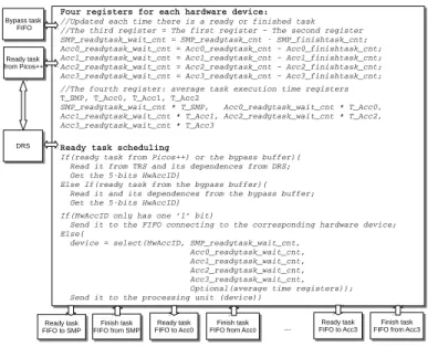
Four registers for each hardware device: //Updated each time there is a ready or finished task //The third register = The first register – The second register SMP_readytask_wait_cnt = SMP_readytask_cnt SMP_finishtask_cnt; Acc0_readytask_wait_cnt = Acc0_readytask_cnt – Acc0_finishtask_cnt; Acc1_readytask_wait_cnt = Acc1_readytask_cnt – Acc1_finishtask_cnt; Acc2_readytask_wait_cnt = Acc2_readytask_cnt – Acc2_finishtask_cnt; Acc3_readytask_wait_cnt = Acc3_readytask_cnt – Acc3_finishtask_cnt; //The fourth register: average task execution time registers T_SMP, T_Acc0, T_Acc1, T_Acc2 SMP_readytask_wait_cnt * T_SMP, Acc0_readytask_wait_cnt * T_Acc0, Acc1_readytask_wait_cnt * T_Acc1, Acc2_readytask_wait_cnt * T_Acc2, Acc3_readytask_wait_cnt * T_Acc3 Ready task scheduling If(ready task from Picos++) or the bypass buffer){ Read it from TRS and its dependences from DRS; Get the 5bits HwAccID} Else If(ready task from the bypass buffer){ Read it and its dependences from the bypass buffer; Get the 5bits HwAccID} If(HwAccID only has one ‘1’ bit) Send it to the FIFO connecting to the corresponding hardware device; Else{ device = select(HwAccID, SMP_readytask_wait_cnt, Acc0_readytask_wait_cnt, Acc1_readytask_wait_cnt, Acc2_readytask_wait_cnt, Acc3_readytask_wait_cnt, Optional(average time registers)); Send it to the processing unit (device)} Bypass task FIFO Bypass task FIFO Ready task FIFO to SMP Ready task FIFO to SMP Ready task from Picos++ Ready task from Picos++ Ready task FIFO to Acc0 Ready task
FIFO to Acc0 FIFO from AccFinish task0 Finish task FIFO from Acc0 Finish task FIFO from SMP Finish task FIFO from SMP DRS DRS Ready task FIFO to Acc3 Ready task
FIFO to Acc3 FIFO from Acc3Finish task
Finish task FIFO from Acc3
...
Fig. 4: Task scheduling to different hardware units a parent has stored its children. Whenever a full condition arises, it checks the state of the first non-executed child. If it has been read, the software support stays at normal state. Otherwise the software support intervenes to avoid a possible deadlock. First, the thread locks the new task buffer and removes all its child tasks. Then, the buffer is reconstructed if it has any remaining tasks (created by other running tasks). Afterwards, either the child tasks removed are directly executed in order by the thread (without allow-ing them to create more tasks) or submitted as a whole to a software task dependence manager. Finally, when the full condition in hardware is cleared, the software support reverts to use hardware for dependence processing. The first option is simpler and keeps the complexity of the software part at bay. The second may allow extra parallelism to be extracted in some corner cases. In any case, tasks can be sent to HwAccs through the bypass task buffer.
3.3 Heterogeneous task scheduling support
To support task scheduling to up to 16 different hardware execution units, a new module called Dependence Reserve station (DRS) is introduced, in addition, the task scheduler (TS) module is modified.
3.3.1 Dependence Reserve Station (DRS)
As in Figure 1, DRS receives new dependence packets from GW. For each of them, DRS saves it into an internal memory indexed by the TRS entry address. When TS wants to schedule a task to a HwAcc, all the dependence memory addresses required can be read sequentially from DRS. This module allows easier and faster access for dependence addresses when scheduling tasks to HwAccs.
3.3.2 Task Scheduler (TS)
TS is mainly responsible for scheduling all the ready tasks to suitable hardware execution units to achieve an earliest finish execution time. Figure 4 shows a simplified scheme of the heterogeneous task scheduling algorithm in TS, assum-ing that there are one SMP and 4 HwAccs, that is, a total of 5 hardware units. Picos++ has one ready and one finished task
queue for SMP, and one ready and finished task queue for each HwAcc. There are two sources of ready tasks: normal ones that are deemed ready by the Picos++ task dependence manager, and bypass tasks. TS checks alternatively from these two sources.
The TS has also four registers associated with each hardware device. Two registers count the number of ready tasks assigned to each HwAcc and the number of finished tasks from this unit. The third register gets the deduction of the previous two registers and indicates the total amount of work still waiting for this unit. Finally the fourth register counts the average task execution time.
Each ready task has a 5bitsHwAccID generated by the target pragmas annotated on each function as shown in Listing 2. ThisHwAccIDcorreponds to a mask that indicates in which accelerators the task can be executed (SMP and
HwAcc0 to HwAcc3 in figure 4). As shown in Figure 4,
when a ready task arrives, TS first checks its hardware mask. If it’s HwAccID indicates only a specific device, it will be scheduled directly to that device. Otherwise, TS compares and selects the one with the least number of waiting work. In the case of multiple devices with identical amount of waiting work, Picos++ selects the one with the higher priority either because this device has more memory bandwidth or is simply faster. The average execution time registers can be enabled when different hardware devices in the system have a big speed gap. In this prototype, the priorities of different hardware are fixed and are based on the infrastructure generated: the HwAcc3 has the highest and the SMP has the lowest priority. For systems that have different connections and hardware devices, the priorities can be modified to suit the characteristics of the system, thus achieving a better performance. This scheme has a small hardware cost, and it balances the workloads well among different hardware devices.
In Figure 1, for each ready task from TRS (R1), TS reads it and might schedule it to SMP (R2). If not, then TS reads all its dependences from DRS (R3) and schedules it to a HwAcc (R4). For a bypass task (R1’), TS gets all its dependences from the bypass task buffer in memory and schedules it to a HwAcc (R4). When a task in the HwAcc finishes, TS retrives it through FIFO queue (F5) to update the Picos++ internal TDG, and also notifies it to the SMP through the ready task buffer in the main memory (F6)
4
E
XPERIMENTALS
ETUP ANDB
ENCHMARKS 4.1 Experimental SetupPicos++ has been coded in VHDL and tested in a Xilinx hardware platform. Its communication logic and all the HwAccs have been coded in C with Vivado HLS directives. The final system designs have been synthesized with Vivado 2016.3. The hardware platform contains a Zynq Ultrascale+ MPSoC Chip XCZU9EG [16]. It includes the Application Processing Unit (APU) with 4 ARM Cortex-A53 cores at 1.1GHz and a FPGA operating at a frequency from 50 to 300MHz, with 4GB DDR4 main memory.
The evaluation of Picos++ is done using the task-based parallel programming model OmpSs [2], it is supported by the source-to-source Mercurium compiler and the Nanos++ runtime system. In this paper, the Picos++ runtime uses the
same task creation mechanism as the Nanos++ runtime, but uses hardware for task dependence analysis and scheduling. We also use performance tools Extrae and Paraver [17] to analyze the application behavior in our system.
Sequential and parallel execution time of OmpSs appli-cations are obtained in the system running Ubuntu Linux 16.04. Each execution has been run for 5 times, and the median value is used.
4.2 Benchmarks
4.2.1 Synthetic and Real Benchmarks
A brief description of the benchmarks follows:
TestFreecreates N tasks with M dependences. Each task has the same execution time T and all of them can be exe-cuted in parallel (tasks are independent of each other). This benchmark is designed to illustrate the processing capacity of Picos++ in the case of an application with embarrassing parallelism.
TestChaincreates N tasks with M dependences, each of execution time T. Each task is the consumer of the previous task, and the producer of the next task. This benchmark is designed to show the worst case, as it has no parallelism at all and suffers the communication latency for offloading task dependences to hardware.
TestNested creates 16 parent tasks. The first 15 tasks have 2 dependences per task but they are independent from each other. Each task (parent task) creates an inout chain of M child tasks, and each child task can be configured to create its own nested tasks. This inout chain is implemented by using the first dependence of each parent. The 16th parent task has 15 dependences that depend on all the previous 15 parent tasks by using their second dependence. This benchmark with configurable nesting levels of tasks and configurable child tasks per parent is constructed to test the nested task support.
Cholesky Factorization computes A = LL’, with A an
n×nmatrix and L lower-triangular.
Multisort sorts the input arrays using the divide and conquer method as can be seen in Listing 1.
Matmulis matrix multiplication. It calculates the multi-plication of two matricesC=AB.
TABLE 1: The characteristics of real benchmarks Name Configs #Tasks Seq time(us) Latency(us)
Matmul (2K, 32) 262144 6820850 26 (2K, 64) 32768 5463956 167 (2K, 128) 4096 5435528 1327 Cholesky (2K, 32) 45760 1232664 27 (2K, 64) 5984 1087485 182 Multisort (1M, 256, 256k) 9565 395594 41 (2M, 512, 512K) 9565 832882 87 (1M, 1K, 512K) 2397 407648 170
For real benchmarks [18], Table 1 shows the number of tasks, sequential execution time and task latency (granu-larity) in microseconds of the applications evaluated with different problem and block size. In the case of Multisort application, column Configs indicates the problem, minimal sort and merge size. During sequential and parallel exe-cution, the non-recursive tasks of Matmul and Cholesky that are executed in threads use Openblas. In the case of Multisort, the non-recursive basic sort tasks are executed in threads usinglibc qsort.
TABLE 2: Characteristics of HwAccs in XCZU9EG
Name HWACCs Latency
B 18Kb DSP48E FFs LUTs us fgemm32 68/3.7% 160/6.4% 19771/3.6% 15559/5.7% 27 fsyrk32 36/2.0% 160/6.4% 19822/3.6% 16149/5.9% 63 ftrsm32 36/2.0% 104/4.1% 11482/2.1% 10875/4.0% 67 fpotrf32 10/0.6% 22/0.9% 3487/0.6% 3302/1.2% 168 fgemm64 74/4.1% 160/6.4% 23887/4.4% 30032/11.0% 126 fsyrk64 42/2.3% 160/6.4% 23849/4.4% 30727/11.2% 270 ftrsm64 42/2.3% 250/9.9% 28734/5.2% 25753/9.4% 314 fpotrf64 28/1.5% 22/0.9% 3514/0.6% 3350/1.2% 981 fmatmul32 68/3.7% 162/6.4% 20106/3.7% 14671/5.4% 27 fmatmul64 138/7.6% 322/12.8% 38770/7.1% 27668/10.9% 105 fmatmul128 287/15.7% 642/25.5% 76147/13.9% 54462/19.9% 497 sort256 68/3.7% 0 20106/3.7% 14671/5.5% 5 sort512 138/7.6% 0 38770/7.1% 27668/10.1% 26 sort1024 159/8.7% 0 47034/8.6% 71124/26.0% 92
TABLE 3: Hardware Resource and Power Consumption Name FPGA resource Power
BRAM18Kb DSP48E FFs LUTs Watts XCZU9EG 1824 2520 548160 274080
Picos++ 87/5.0% 0 5478/1.0% 9793/4.0% 0.07 Comm. Logic 2/0% 0 3421/0.6% 4244/1.0% 0.03
APU Watts
4 ARM Cortex-A53s - - - - 1.4
4.2.2 HW Functional Accelerators (HwAccs)
Table 2 shows the hardware cost (absolute number of logics and percentage of FPGA used) of different HwAccs, and their latencies in microseconds for executing a task. All the accelerators are synthesized using 200 MHz clock. In the Cholesky application there are four different HwAccs: fgemm, fsyrk and ftrsm and fpotrf that correspond to its four different kernels. Matmul and Multisort applications have only one type of HwAccs each, fmatmul and sort, respectively.
4.3 Hardware Resource and Power Consumption Table 3 shows the on-chip resource utilization and power consumption of Picos++ on the Zynq Ultrascale+ XCZU9EG chip [16]. The resource usage is obtained from Vivado post-implementation reports. Picos++ and its communication logic use around 5% of the FPGA resources. This is im-portant as not only it is small in order to be feasible to integrate it into multicore processors with very low cost, but also it allows us to build a highly heterogeneous platform combining Picos++ with other HwAccs. The 4 ARM Cortex-A53 cores take around 93.3% of the whole chip power (1.4W out of 1.5W). Picos++ and its data communication logic only consume 0.1W.
The power consumption is measured through dedicated hardware registers in three main hardware parts: FPGA, APU and the main memory DDR4. Energy consumption is calculated by integrating the total power consumed by the three parts along the application execution time.
5
P
ERFORMANCE ANDE
NERGYC
ONSUMPTION 5.1 Task and Dependence Repetition RateTable 4 shows the task and dependence repetition rates (rrTask and rrDep) of the software-only runtime and Pi-cos++ measured in 100MHz clock cycles. TestFree and TestChain with 65536 empty tasks (zero execution time) are used to avoid the influence of task execution time,
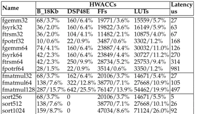
(a) TestFree (b) TestChain (c) TestFree 15 deps (d) TestChain 15 deps
Fig. 5: Execution time and relative speedup of TestFree, TestChain with 4 threads TABLE 4: Task, Dependence Repetition Rate in cycles
Testcase TestFree TestChain
Number of dependences 1 15 1 15 HW-only rrTaskrrDep 2424 243 3516 35 34823 SW-only 2trrTask 1175 5281 1668 3095
rrDep 1175 352 1668 206 SW-only 4trrTaskrrDep 1055 5272 1706 31181055 352 1706 208 Picos++ 2t rrTask 731 855 1251 1419
rrDep 731 57 1251 96 Picos++ 4t rrTask 582 716 1250 1406
rrDep 582 48 1250 94
and different number of dependences are used to study its impact. Row HW-only shows results without any communi-cation latencies or software runtime overhead (task creation and scheduling) in Picos++. Note that the communication between the processors and Picos++ costs around 300 clock cycles for the full life cycle of a task. Row SW-only 2t and 4t show results obtained from real executions by using SW-only runtime with 2 and 4 threads. Similarly Row Picos++ 2t and 4t shows real execution results obtained by using the Picos++.
With HW-only, each task and dependence only takes a few cycles to be processedand only increases slightly when increasing the number of dependences. For example, tasks with 1 dependence in TestFree and TestChain are processed in 24 and 35 cycles respectively while with 15 dependences, they are processed in 243 and 348 cycles. The dependence repetition rate is quite steady for different dependence pat-terns ranging from 16 to 23 cycles. This is due to the fact that Picos++ pipelines the processing of all the dependences of a task. Tasks that are processed through the bypass task buffer have the same repetition rate as TestFree tasks with no dependences.
Althouth data communication has a big impact over system performance as it can be seen in Picos++ rows in Table 4, the two observations about HW-only hold true for Picos++ with 2t and 4t. As a result, there is a clear speed up of managing task dependence analysis in hardware than in software.
5.2 Synthetic Benchmarks
5.2.1 Performance Impact of the Number of Dependences
Figure 5 shows results of TestFree and TestChain. All the fig-ures have two Y-axis, the left one (in bars) indicating the exe-cution time in seconds, and the right one (in lines) showing the relative speedup of Picos++ against the software-only runtime with 1 or 4 threads. The left two diagrams in Fig-ure 5 display these two benchmarks with 65536 empty tasks
(a) 4 child in each parent task (b) 16 child in each parent task
Fig. 6: Time and speedup of TestNested with 4 threads (tasks with 0 execution time), and with different number of dependences. Picos++ and SW-only are using the same task creation and scheduling mechanism, therefore with empty tasks the results highlight the dependence analysis cost difference and the communication overhead in Picos++. There are two key observations. First, Picos++ maintains a nearly equal performance from 1 to 15 dependences per task. Second, it has a much lower dependence analysis cost. For 15 dependences and TestFree, where there is full parallelism, Picos++ is 7.5x faster than SW-only using 4 threads. In the case of the TestChain, for the same number of dependences and where there is no parallelism at all, Picos++ still is up to 2x faster than the SW-only runtime.
5.2.2 Performance Impact of the Task Granularity
The two right diagrams of Figure 5 show results for the same number of tasks, 15 dependences per task and a range of task sizes (X-axis) going down from 1ms to 530ns. As it can be seen, the smaller the task size, the higher speedup Picos++ has when compared to the SW-only runtime. In particular Picos++ is 8x and 2.5x faster than SW-only for TestFree and TestChain respectively.
5.2.3 Support and Performance of Nested Tasks
Figure 6 shows results of TestNested with 4 and 16 levels of nested child tasks per parent task. On the one hand, results show that Picos++ can deal with nested tasks. On the other hand, Picos++ also benefits from fine-grained nested task: with smaller task sizes Picos++ is faster than the SW-only runtime.
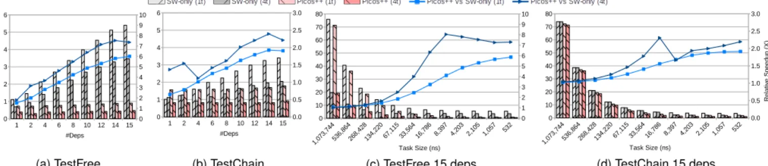
5.2.4 Scalability with 15 Accelerators
Figure 7 shows three sets of results for TestFree with 65536 tasks and with 15 dependences per task. The figures show the total execution time (bars, in the left Y-axis) of using Picos++ and SW-only runtimes and the relative speedup comparing these two (lines, in the right Y-axis). The X-axis
(a) Picos++ at 50Mhz (b) Picos++ at 100Mhz (c) Picos++ at 200Mhz
Fig. 7: Execution time and speedup of TestFree by using Picos++ and SW-only with 15 HwAccs in each set shows a decreasing task size from 0.5ms to 160ns.
From left to right, the three figures show Picos++ operating at 50, 100 or 200MHz respectively. In this experiment there are in total 15 HwAccs operating at 200MHz while all the SMP cores operate at 1.1GHz. For each set, there are also results for using either sequential or parallel task creation mechanisms in the cores.
TestFree with sequential creation used to obtain the data in Figure 7 is the same that has been used in the previous sections, where only one thread creates all the new tasks. We have realized that in this particular experiment, as there were so many (15) fast HwAccs the element limiting the execution time was in fact the task creation. In order to ease this limitation we have implemented the same program where three of the available threads create the tasks in parallel (using nested tasks). The remaining thread is used to process all the finished tasks as this is the fastest thread combination to execute this benchmark.
As it can be seen from the total execution time (bars) in Figure 7, the SW-only runtime benefits from the parallel task creation. However with task sizes smaller than 327,680ns (0.3ms) it is unable to execute the program faster (grey bars). On the other hand, when operating at 200MHz, Picos++ is able to decrease the execution time with task sizes of around 10,240ns (0.01ms) resulting in a 25x speedup against the SW-only runtime.
It can be also seen that, in the first plot where Picos++ is operating at 50MHz, the execution time of using sequential and parallel task creation is the same. This is because there is a huge frequency gap between the cores (1.1GHz) and Picos++ (50MHz). Although it is around 10x faster than the SW-only runtime it is not fast enough to serve the parallel task creation with 4 cores at full speed.
Moving to the second plot where Picos++ operates at 100MHz, it starts to take advatage of parallel creation. Now Picos++ operates at twice the frequency than the previous one and thus should obtain half of the execution time. This holds true for the parallel task creation, but not for the sequential one, which means with 100MHz Picos++ is able to fully serve the sequential task creation with 1 core (in this case software task creation is the bottleneck).
Finally, looking at the 200MHz results, the execution time with sequential task creation remains the same as expected. However, the execution time of parallel task cre-ation is roughly one third of that with Picos++ running at 100MHz. This means that Picos++ running at 200MHz is able to deal with parallel task creation with 4 cores at full speed, and the software becomes again the bottleneck. Extrapolating these results, Picos++ operating at the same
speed as the cores (at 1.1GHz) should be able to serve around 22 cores creating tasks at full speed with tasks as small as 1861ns executing all at the same time.
To sum up briefly, Picos++ is able to take advantage of fine-grained parallelism, and it is able to achieve a 25x speedup over the software-only runtime with 15 HwAccs. More importantly, we can safely conclude that, with more hardware resources and a higher frequency design, Picos++ is able to achieve even higher performance for a much larger range of task granularities.
5.3 Real Benchmarks
5.3.1 Performance Impact of the Task Granularity
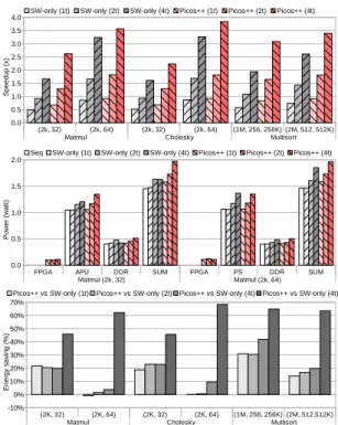
Figure 8 shows the speedup, power consumption, and en-ergy savings of applications using fine-grained tasks that are executed only in SMPs. Each application in the X-axis shows two sets of problem and block size per application (their task sizes are shown in Table 1). In Y-axis the results show the results obtained by SW-only and Picos++ with 1 to 4 threads. In this experiment, Picos++ is operating at 100MHz and SMP is operating at 1.1GHz.
As can be seen, Picos++ exceeds SW-only in speedup in all the cases. For example, Picos++ reaches a 3.6x speedup in Matmul with block size 64 and a 3.4x speedup in Multisort with sort size 512. The global performance obtained when using a larger block size in Matmul and Cholesky is better because there are far less and larger tasks to manage. How-ever this is due to the limited number of threads available in the system. With more threads Picos++ shall be able to obtain a much higher performance with block size 32. Despite that, we can still observe that the gap between Picos++ and SW-only enlarges as the task size becomes smaller from block size 64 to 32. For example, with Matmul with block size 32, Picos++ obtains 1.5x speedup versus SW-only; Similar gap can be observed in both Cholesky and Multisort.
Figure 8 shows the power consumption of the system during Matmul execution. Other applications have simi-lar patterns, therefore only Matmul is shown as a rep-resentative. As can be seen, the power consumption of APU is proportional to the number of threads, and that of DDR is steady during all the executions. Both SW-only and Picos++ use similar power in these two parts. For FPGA, using Picos++ consumes 0.1 watt more power. This slight consumption increase translates to the SUM (SUM=FPGA+APU+DDR) part.
Figure 8 also shows the energy consumption of all the applications by using Picos++ versus the SW-only runtime
Fig. 8: Results of applications with fine-grained SMP tasks or sequential executions. When compared to the sequential version, Picos++ runtime using 4 threads saves more than 60% of energy for all the applications, mainly due to the faster execution. When compared to the SW-only runtime, with more threads available and smaller task sizes, Picos++ saves a much higher amount of energy: 22%, 24% and 42% for the three applications.
Applications with medium size tasks can also benefit from using Picos++. For example, Picos++(4t) is faster ex-ecuting Multisort with sort size 1K with a 3.6x speedup than SW-only(4t) that only reaches a 3.1x against sequential. Correspondingly, with Multisort, Picos++(4t) saves 20% and 65% of the energy consumption compared to SW-only(4t) and sequential execution.
5.3.2 Performance of Heterogeneous Task Scheduling
Figures 9a, 9c and 9e show the speedup obtained in the three analyzed applications when comparing the parallel runtimes (Picos++ and SW-only) against the sequential execution. The sequential execution is obtained by using one core in the SMP. The legend SW-only(Na) indicates results obtained by using the software-only runtime with tasks that are not executed in threads but in N HwAccs. Legend SW-only(Na+4t) indicates results obtained by using the software-only runtime with tasks that are executed in both 4 threads and N HwAccs. The same logic applies to the legends for Picos++. Special attentions should be paid for the legend with ”*” symbols. For example, with Matmul block size 128 and Multisort sort size 1K in Figure 9a and 9e, it means that the system contains only 3 instead of 4 HwAccs due to the limited capacity of the FPGA that can not hold 4 of these accelerators. It is also worth to mention that with Cholesky in Figure 9c, two different sets of HwAccs are used, hence the SW-only(4a+4t) and (4g+4t). This will be explained later.
As can be seen, using a system with HwAccs results in a much higher speedup than using SMP threads only.
TABLE 5: The number of tasks executed in different hard-ware in the Picos++ system
Size Case #SMP #HWACC0 #HWACC1 #HWACC2 #HWACC3
(2k, 32) 4a 0 41664 2016 2016 64 4a+4t 17992 23839 2015 1850 64 4g+4t 4096 10300 10371 10451 10542 (2K, 64) 4a 0 4963 496 496 32 4a+4t 2344 2667 493 448 32 4g+4t 1024 1209 1235 1258 1258
For a brief comparison, in Figure 9a Matmul Picos++(4a+4t) achieves up to 11.2x speedup while using only SMP threads (in Figure 8) the speedup obtained is only 3.6x. A similar behavior can also be observed in the other two applications. In addition, Picos++ is much better at managing hybrid system than the software-only runtime. With tasks that can be executed in both FPGA and SMP threads, for example, for Choleksy, Picos++(4a+4t) reaches up to 3x speedup while SW-only displays 1.7x. Even better, the implementation of Picos++(4g+4t) reaches up to 6.7x while the software-only runtime only achieves 4.8x speedup. Similarly good results can be seen for Matmul and Multisort.
Furthermore, the gap between Picos++ and the software-only runtime enlarges as the task size becomes smaller (corresponding task sizes can be found in Table 2). For Matmul, the performance gap obtained when going from block size 128 to 32 enlarges from 1.1x to 2.7x faster; for Cholesky, the gap when decreasing from block size 64 to 32 goes from 1.4x to 2.7x and for Multisort, the gap grows from 1.6x to 7.6x.
Correspondingly, Figures 9b, 9d and 9f show the energy savings of using Picos++ instead of the software-only run-time or sequential executions. As can be observed, with a smaller task size and more execution units, Picos++ saves much more energy. For example, for Matmul with block sizes 64 to 32, Picos++ saves from up to 27% to 64% respectively; in addition with Picos++ vs SW-only(1a) to (4a+4t), Picos++ energy saving raises from 31% to 67%. With Multisort, the task sizes of 256 and 512 are very close. As a result, Picos++ saves a similar amount of energy for both granularities, up to 90%. For Multisort, it can also be seen that the speedup and energy savings obtained by using 1 to 4 HwAccs do not vary much for the different task sizes. This is because that most of the execution time is spent on unraveling the nested layers. As a result there are simply not enough tasks to feed the HwAccs. With Cholesky with block size 32, an energy saving of up to 68% of Picos++ over SW-only (4g+4t) can be observed.
As mentioned earlier, two different sets of HwAccs (4a and 4g) were used for Cholesky executions shown in Figure 9c. Table 5 shows the number of tasks that have been executed in the different hardware for three cases: The first case (4a) is for using only 4 different HwAccs, corresponding to the four kernel functions of Cholesky: gemm, syrk, trsm and portf. Therefore each task can only be executed in one of these accelerators. As a result, in this case with block size 32 the software-only runtime is slower than the sequential version, however Picos++ is able to obtain a small performance improvement. The second case (4a+4t) allows each task to be executed in one specific accelerator or in the threads. The third case (4g+4t) uses four instances of the same HwAcc (gemm) and uses the threads for the
other tasks. In the first case, there is no parallelism for the same type of tasks during execution, and the dominating number of gemm tasks also dominates the total execution time. By allowing gemm tasks to execute in SMP threads in the second case, nearly half of the gemm tasks are balanced between SMP and HwAcc0, which improves 2x the performance comparing to the first case. For the third case, by employing four instances of gemm accelerators Picos++ further balances the workloads and gains a 4x speedup compared to the first case.
(a) Matmul speedup (b) Matmul energy savings
(c) Cholesky speedup (d) Cholesky energy savings
(e) Multisort speedup (f) Multisort energy savings
Fig. 9: Speedup and energy savings of applications
5.3.3 Gflops and Gflops per watt
Figure 10 shows the Gflops (Y-axis) obtained by both the software-only and Picos++ runtimes when computing Mat-mul with 3 HwAccs of block size 128x128 each. From left to right, and for both the software-only and Picos++ runtimes, the bars show results when using only HwAccs for task execution and HwAccs and 1, 2, 3, or 4 SMP threads to execute tasks. Tasks executed in the SMP use the optimized version of the OpenBlas sgemm (single precision Matmul) implementation. The threads operate at 1.1GHz, Picos++ at 100MHz and HwAccs at 300MHz. It is important to state that this configuraction (3 HwAccs of block size 128x128) is the one that obtains the best performance for this problem in this system when using the software-only runtime, so we selected this configuration to compare against Picos++.
The software-only runtime requires 2 threads to manage the task scheduling for 3 HwAccs, which causes
perfor-Fig. 10: Matmul Gflops with 3 FPGA accelerators mance degration when 3 or 4 SMP threads are enabled for task execution as the same thread is used both to compute tasks and manage HwAccs. On the other hand, Picos++ increases the application performance. The small slowdown when using one additional SMP thread is due to a scheduling decision for the last task to be executed in SMP thread rather than waiting for the HwAccs. This is translated in a load unbalance between them since HwAccs are much faster than threads for task execution. However, with more threads in the system, this unbalance disappears. This unbalance with one thread could also be solved by enabling the average task execution time policy in task scheduling in Picos++ as mentioned in earlier sections.
Picos++ obtains more Gflops when more hardware re-sources exist in the system and better performance than the software-only runtime. The software-only runtime achieves up to 39.6 Gflops while the Picos++ runtime obtains up to 49 Gflops. The whole system (with the Picos++ runtime) executing this problem has a power consumption of only 5.74 watts, which translates into 8.54 Gflops per watt. To give an meaning to this value, the same application was run on different machines. A Intel i5-3470 core (with 4 threads at 3.20GHz) achieves 0.51 Gflops per watt. A Intel Xeon E5-2020 V2 (with up to 24 threads at 2.1GHz) achieves 4.14 Gflops per watt and a Intel i7-4600U core (with up to 4 threads at 2.1GHz) achieves 4.75 Gflops per watt.
5.3.4 Scaling Up the Number of HwAccs
Figure 11 shows the speedup of using Matmul with problem size 2kx2k and block size 32x32 with up to 12 HwAccs (the maximum number of fmatmul HwAcc with this block size that can be fit inside the FPGA). There are two sets of results corresponding to Picos++ working at 100MHz and 200MHz. For each set, there are four bars corresponding to the speedup of Picos++ over sequential and the speedup of Picos++ over the software-only runtime. In addition each case is measured with sequential and parallel task creation. The X-axis shows an increasing number of HwAccs used in the system.
(a) Picos++ at 100Mhz (b) Picos++ at 200Mhz
Fig. 11: Speedup of matmul (2k, 32) by using Picos++ runtime with up to 12 HwAccs
3,529,008 ns 0 ns
Tasks and dependencies@Picos++_12accs_1k_32.prv
Main Parallel task creation Thread 1
Thread 2 Thread 3 Thread 4
FPGA task management (a) by using Picos++ runtime with 12 HwAccs
3,529,008 ns 0 ns
Tasks and dependencies@SW-only_12accs_1k_32_throttle.prv
Main Parallel task creation FPGA task management Thread 1
Thread 2 Thread 3 Thread 4
(b) by using SW-only runtime with 12 HwAccs
Fig. 12: Task Instances of Matmul 2k, 32 execution In Figure 11, when comparing Picos++ against the se-quential execution it can be seen that when executing Pi-cos++ at 100MHz, using parallel task creation results in a small boost of the performance of Picos++, allowing it to scale from 6 to 8 HwAccs and obtaining from 3.72x to 5x speedup. The applications scales up to 10 HwAccs and the speedup improves from 4.8x to 8.21x when running with Picos++ at 200MHz. Both the size of the tasks (27 ns in Ta-ble 2, corresponding to the fmatmul32 HwAcc at 200MHz) and the maximum number of HwAccs that Picos++ is able to manage at the same time are coherent with the results shown in Figure 7. When Picos++ is compared against the software-only runtime, it can be seen that Picos++ executed at 200MHz and with parallel task creation achieves a 16.2x speedup.
To summarize, Picos++ is good at managing heteroge-neous tasks when taking into account both performance and energy savings. This is partly due to the fast dependence analysis and nested task support, but also a new factor weights in. The heterogeneous task scheduling in hardware plays an important role in this case as it not only balances the workload among all the devices, but also brings the ready-to-execute tasks much closer to the HwAccs in FPGA and reduces thread contention while the software-only run-time is heavily burdened by such overhead.
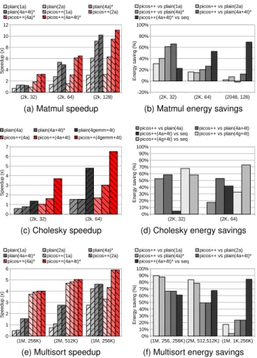
To further explain this effect, Figure 12 shows two different traces of the same Matmul application (problem size and block size), with parallel task creation, using the Picos++ runtime at 200MHz (Figure 12a) and the software-only runtime at 1.1GHz (Figure 12b), with 12 HwAccs.
As can be seen, the execution time is much shorter when using Picos++ than the software-only runtime. When exam-ined closely, the biggest difference between these two traces lays in the FPGA task management, as it dominates the execution time in the software-only runtime. This is because Picos++ directly manages the scheduling and finalization of FPGA tasks, therefore the FPGA task management only concerns the deletion of task descriptors in the software part of the runtime. For the software-only runtime, however, the threads are required to manage scheduling, finalization and the deletion of FPGA tasks. This overall management, which is expensive and also provokes contentions, is translated into a significant increment of the management overhead and the execution time of the application. This, together
Thread 1 Thread 2 Thread 3 Thread 4
omp_trsm
46,000,924 ns main omp_potrf omp_syrk 51,756,839 ns
(a) Tasks instances
Thread 1 Thread 2 Thread 3 Thread 4
Send new task
zoom
Send new task Polling for ready/
executed HW task Send finished task
46,000,924 ns 51,756,839 ns
(b) Picos++ APIs
Fig. 13: Visualization of Cholesky execution
with the faster task dependence analysis in hardware, ex-plains the performance difference between the Picos++ and the software-only runtime.
5.4 Potential Energy Savings Analysis
Figure 13 shows an execution trace of the Cholesky applica-tion executed using Picos++ and 4 gemm HwAccs. Similar behaviors have been observed for other real applications. This trace shows, for clarity, an execution of a small problem size 256x256 with block size 64x64, which has 20 tasks in total. Figure 13a shows the tasks that each thread is executing at a given moment. As it can be seen, gemm tasks are not shown as they are executed by the HwAccs instead of by the threads. Figure 13b shows the Picos++ activities performed by each thread in the same execution. As it can be seen any thread at a given moment is executing either a SMP task, or a Picos++ activity or nothing. In addition, we have zoomed in a region in Figure 13b to show the series of sequential pollings the threads perform due to the lack of available tasks. These polling sequences are not continous.
Figure 13a shows the duration of each task: main, omp potrf, omp syrk and omp trsm. Thread 1 (T.1 horizon-tal timeline in the figure) is the main thread and launches the main function (shown in Figure 13a), which creates new tasks (shown in the thread activity in Figure 13b), at the beginning of the trace. During this time threads 2, 3 and 4 are actively polling for ready/executed HwAcc tasks. The first SMP task that was deemed ready by Picos++ is omp potrf, and it was scheduled and executed in thread 2 in Figure 13a. After omp potrf, three instances of omp syrk and then, three instances of omp trsm are executed in threads 2, 3 and 4. Once a task finishes its execution in a thread, this thread sends a finished task to Picos++. At the end of each task in Figure 13a, it can be seen a finished task send action in Figure 13b. For all the tasks that are executed in FPGA, there is a finished HwAcc task sent from Picos++ to notify the threads to delete the task descriptor.
In Figure 13a, only a portion of time is spent executing useful work, the rest is wasted on idle polling for ready/ex-ecuted HwAcc tasks as shown in Figure 13b. Table 6 quan-tifies the percentage of time of all the useful functions in the threads and HwAccs for a real problem with a bigger problem size 2Kx2K. As it can be seen in theTaskscategory, the main task is executed mainly in Thread 1 and consumes 97% of its time. The other threads execute mainly the potrf, syrk and trsm functions when they are available. Gemm