Rapid Combined
T
1
and
T
2
Mapping Using Gradient
Recalled Acquisition in the Steady State
Sean C.L. Deoni,
1,2Brian K. Rutt,
1–3and Terry M. Peters
1–3*
A novel, fully 3D, high-resolution T1 and T2 relaxation time
mapping method is presented. The method is based on steady-state imaging withT1and T2information derived from either
spoiling or fully refocusing the transverse magnetization follow-ing each excitation pulse.T1is extracted from a pair of spoiled
gradient recalled echo (SPGR) images acquired at optimized flip angles. ThisT1information is combined with two refocused
steady-state free precession (SSFP) images to determineT2.T1
andT2accuracy was evaluated against inversion recovery (IR) and spin-echo (SE) results, respectively. Error within theT1and T2maps, determined from both phantom and in vivo
measure-ments, is approximately 7% forT1between 300 and 2000 ms
and 7% forT2between 30 and 150 ms. The efficiency of the
method, defined as the signal-to-noise ratio (SNR) of the final map per voxel volume per square root scan time, was evaluated against alternative mapping methods. With an efficiency of three times that of multipoint IR and three times that of multi-echo SE, our combined approach represents the most efficient of those examined. Acquisition time for a whole brainT1map (25ⴛ25ⴛ10 cm) is less than 8 min with 1 mm3isotropic voxels.
An additional 7 min is required for an identically sizedT2map
and postprocessing time is less than 1 min on a 1 GHz PIII PC. The method therefore permits real-time clinical acquisition and display of whole brainT1andT2maps for the first time. Magn
Reson Med 49:515–526, 2003.©2003 Wiley-Liss, Inc.
Key words:T1;T2; SSFP; SPGR; relaxation time mapping; rapid
volumetric imaging
A fast and accurate method of determining the longitudi-nal,T1, and transverse,T2, relaxation constants on a voxel-by-voxel basis has long been a goal of MRI scientists. Rigorous characterization of T1 and T2 may allow for greater tissue discrimination, segmentation, and classifica-tion, thereby improving disease detection and monitoring, as well as enhancing the images used for image-guided surgical procedures. Absolute determination ofT1andT2 is clinically useful in areas such as in-flow perfusion stud-ies (1) and dynamic contrast agent studstud-ies (2), as well as in the diagnosis of epilepsy (3) and in determining the sever-ity of Parkinson’s disease (4). Therefore, a method that
permits simultaneousT1andT2determination in a rapid manner would be useful in a wide range of imaging appli-cations.
In order to be clinically useful for neuroimaging appli-cations,T1andT2maps should be of high resolution, with a voxel volume less than 1 mm3, and have low noise. Imaging time should be less than 30 min for a large volume (25 ⫻ 25 ⫻ 10 cm) with minimal postprocessing time. Ideally, postprocessing would be performed at the scanner console.
Despite the long acquisition times, the principal meth-ods forT1andT2mapping remain inversion-recovery (IR) and saturation-recovery (SR) for T1, and spin echo (SE) and multiple or fast spin echo (mSE, FSE) forT2. Although alternative methods (5–9) have been developed to rapidly and accurately determineT1orT2, the low signal-to-noise ratio (SNR), lengthy reconstruction time, or special hard-ware requirements associated with these newer methods reduce their appeal.
The variable nutation angle method originally intro-duced in 1974 (10) and investigated by a number of au-thors (11–14) calculatesT1with an accuracy similar to that achieved by the IR and SR techniques, but with a signifi-cant decrease in acquisition time. The sequence involves establishing a spoiled steady state followed by the collec-tion of spoiled gradient echo (SPGR) images over a range of flip angles. This generates a signal curve that depends on T1and which is easily linearized, allowing for quick T1 determination. We believe that this method is the most appropriate for use in 3D T1 mapping due to the rapid acquisition, high measurement precision, and efficient postprocessing.
First described some 40 years ago (15), the steady-state free precession (SSFP) pulse sequence has received atten-tion recently as a high-speed, highly efficient imaging method. The underlying sequence is similar to SPGR, but differs in one respect: both longitudinal and transverse magnetization are brought into dynamic equilibrium through the application of ␣ pulses and fully refocusing the transverse magnetization prior to each excitation pulse. Collecting SSFP images over a range of flip angles yields a signal curve that is a function of bothT1andT2 (16). We demonstrate in this article that this signal curve can also be cast into a linear form, allowing for rapid determination ofT2, providedT1is known. Thus, perform-ing variable nutation angle SPGR and SSFP experiments sequentially allows us to determine bothT1andT2 relax-ation times significantly faster than is possible with exist-ing methods.
In this article we introduce the use of variable nutation SPGR and SSFP for combinedT1andT2quantification and examine the parameters of SPGR and SSFP that influence the precision of theT1andT2estimates. Specifically, we 1Imaging Research Laboratories, Robarts Research Institute, London,
On-tario, Canada.
2Department of Medical Biophysics, University of Western Ontario, London,
Ontario, Canada.
3Department of Diagnostic Radiology and Nuclear Medicine, University of
Western Ontario, London, Ontario, Canada.
Grant sponsor: Canadian Institutes for Health Research; Grant numbers: MT-11540; GR-14973; Grant sponsors: University of Western Ontario; Gen-eral Electric Medical Systems.
*Correspondence to: Terry M. Peters, Imaging Research Laboratories, Ro-barts Research Institute, P.O. Box 5015, 100 Perth Drive, London, Ontario N6A 5K8, Canada. E-mail: [email protected]
Received 19 February 2002; revised 16 October 2002; accepted 20 October 2002.
DOI 10.1002/mrm.10407
Published online in Wiley InterScience (www.interscience.wiley.com).
examine the role of repetition time and the optimization of the flip angles for high-speed mapping. Following these optimizations, we show how the method, using SPGR and SSFP data acquired from just two flip angles each, can be used for rapid 3D volumetric T1and T2 mapping of the brain. Finally, we characterize the efficiency of our opti-mized method by comparing it with existing conventional and accelerated methods. Based on a metric of SNR effi-ciency in the final T1 and T2 maps, we show that the proposed method is superior to the traditional approaches and allows fully 3D combinedT1and T2mapping to be achieved in a clinically acceptable scanning time. We have extended the naming convention originally used in (11) to refer to our optimized variable nutation SPGR and SSFP; we call the former approach DESPOT1 and the latter DES-POT2, reflecting theT1andT2mapping properties of these techniques.
THEORY
Basic DESPOT1 Theory
A thorough theoretical description of SPGR has been given previously (5), so we simply state that the measured SPGR signal intensity (SSPGR) is a function of the longitudinal
relaxation time,T1, repetition time,TR, flip angle,␣, and a factor which is proportional to the equilibrium longitudi-nal magnetization,Mo: SSPGR⫽ Mo共1⫺E1兲sin共␣兲 1⫺E1cos共␣兲 [1] whereE1⫽exp(–TR/T1).
By holdingTRconstant and incrementally increasing␣, a curve characterized byT1is generated. As demonstrated in Ref. 5, these data can be represented in the linear form, Y⫽mX⫹bas:
SSPGR
sin共␣兲⫽E1 SSPGR
tan共␣兲⫹Mo共1⫺E1兲 [2] from which the slope, m, and the Y-intercept, b, can be estimated by linear regression, allowingT1and Moto be
extracted:
T1⫽⫺TR/ln共m兲 [3a] Mo⫽b/共1⫺m兲. [3b]
Basic DESPOT2 Theory
The general SSFP sequence involves the repeated applica-tion of excitaapplica-tion pulses with flip angle␣at aTRmuch less than eitherT1orT2. With perfect refocusing of the spins, a steady state is achieved in both the longitudinal and transverse magnetizations. The signal intensity (SSSFP) is
therefore expressed as a function of the tissueT1andT2 relaxation times, TR, ␣, andMo. However, the literature
contains multiple forms of the SSFP signal equation (15,17–21). In our case, whereTRis kept short (less than 10 ms) and the RF pulses are alternated by 180°, the
equation derived by Perkins and Wehrli (18) is the most appropriate: SSSFP⫽ Mo共1⫺E1兲sin共␣兲 1⫺E1E2⫺共E1⫺E2兲cos共␣兲 [4] whereE2⫽exp(–TR/T2).
Holding TR constant and incrementally increasing ␣ generates data that depend on bothT1andT2. Equation [4] can be recast into the linear form Y⫽mX⫹b,giving us:
SSSFP sin共␣兲⫽ E1⫺E2 1⫺E1E2⫻ SSSFP tan共␣兲⫹ Mo共1⫺E1兲 1⫺E1E2 . [5]
IfT1(and henceE1) is known,T2andMocan be calculated
from the values of slope (m) and intercept (b) as:
T2⫽⫺TR/ln
冉
m⫺E1 mE1⫺1冊
[6a]
Mo⫽b共E1E2⫺1兲/共1⫺E1兲. [6b] Optimum DESPOT1 Flip Angles: Numerical Solution Previous authors (12,13), and most notably Wang et al. (14), have investigated the parameters that influence the variable nutation SGPR T1 estimate precision. In their approach they begin with a set of standard flip angles (SA)⫽ {10,20,30…80,90,100°} and examine the effect of alteringTRfor a givenT1. Using this approach, Wang et al. reported that optimum T1 precision occurs when the TR/T1ratio is approximately 1.1:1. They also showed that the precision obtained using 10 flip angles can be achieved using just two optimized angles with a corresponding 5-fold reduction in imaging time. The two optimized an-gles were determined via an iterative method, which min-imized the T1 estimate variance. Unfortunately, their method does not reveal the mechanism that determinesT1 precision. As a result, they do not provide a simple one-step method for determining the two angles.
To determine which two angles to use for a particular TR/T1 combination in a more straightforward manner, consider the estimation of T1from the linearized signal. The two signal intensities provide two points on the re-gression line. If each point suffers the same uncertainty, the further the two points are separated along the line, the better the estimate of slope. This separation along the ordinate can be defined as the normalized dynamic range (DR) of the regression line, given by:
DR⫽ S␣2 Mosin共␣2兲⫺
S␣1 Mosin共␣1兲
[7]
where␣1and␣2are the two flip angles andS␣1andS␣2are
the SPGR signals associated with␣1and␣2.
In our case, the data points do not suffer the same uncertainty; rather, the precision depends on the location of the points along the line and generally decreases as the two points move away from the midpoint (defined by the location of the peak of the signal curve and given by the
Ernst signal (S␣E)). This means that the precision can be
related to the fractional signal of the points (FS).
FS⫽共S␣1⫹S␣2兲/2S␣E. [8]
With the above considerations of the trade-off betweenDR and FS, we propose that optimum T1 precision will be achieved when the product ofDR⫻FSis maximized.
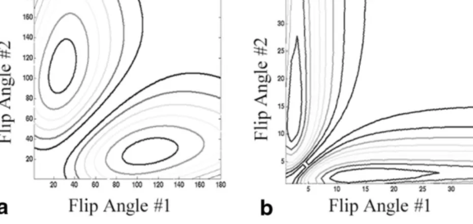
Figure 1a is a resultant plot ofDR⫻FS, from which the ideal angles can be determined. In this example, where we have used the same values as Wang et al. (TR⫽800 ms, T1⫽ 1000 ms), we confirm their prediction of the ideal angles as 29° and 112°. Due to the strong agreement be-tween our results and those of Wang et al., we believe the DR⫻FSproduct can be used to determine the ideal angles for anyTR/T1case.
In our application we are interested in using very low TRvalues, i.e.,⬍5 ms. Results of an analysis similar to the above withTR⫽5 ms andT1⫽1000 ms are presented in Fig. 1b. In this case, the ideal angles are shown to be 3° and 13°, which are quite different from those found in the high TR case. The impact of angle choice is clearly demon-strated in these two examples and stresses the need for a simple method of determining the ideal angles for arbi-traryTR/T1combinations.
Optimum DESPOT1 Flip Angles: Analytical Solution While we have shown that it is possible to determine the two ideal angles by searching for maxima in theDR⫻FS space, the process is time-consuming and so fails to
pro-vide a simple analytical method of determining the ideal angles for arbitraryTR/T1combinations.
Derivation of an analytical prediction of optimal dual SPGR angles requires the following simplifications. By plotting theDR⫻FSproduct over a wide search-space, it becomes apparent that this product is maximized when S␣1⫽S␣2. Therefore, we simplifyFStof:
f⫽S␣1/S␣E⫽S␣2/S␣E. [9]
In Fig. 2a, this new function (DR⫻ f) is plotted against TR/T1andf. Fitting a polynomial for eachTR/T1case and solving for the maximum, we find that over the complete range ofTR/T1investigated the function is maximized at f⫽0.71. Therefore,T1precision is maximized by choosing the flip angles such thatS␣1⫽S␣2⫽0.71S␣E.
We can now derive a general analytical solution for the two ideal angles. ExpandingS⫽f⫻S␣Eusing Eq. [1] we
obtain: sin共␣兲 1⫺E1cos共␣兲⫽ f⫻sin共␣E兲 1⫺E1cos共␣E兲 . [10]
Following the derivation shown in Appendix A, we obtain a solution for the angles as:
␣⫽cos⫺1
冉
f 2E1⫾共1⫺E12兲
冑
1⫺f2 1⫺E12共1⫺f2兲
冊
. [11]FIG. 1. Contour plots of the dynamic range⫻ fractional signal as a function of␣1and␣1for a:TR⫽800 ms andT1⫽1000 ms; the
opti-mum angles are 29° and 112°.b:TR⫽5 ms andT1⫽1000 ms; the optimum angles are 3°
and 13°. Contours span the range [6, 73] ina
and [3, 46] inb.
FIG. 2. a:DR⫻fcalculated over the search-space 0⬍S␣1,2/S␣E ⬍100% and 0⬍TR/ T1 ⬍ 50. Maximum precision occurs when
S␣1,2/S␣E⫽0.71.b:DR⫻fcalculated over
the search-space 0⬍S␣1,2/S␣E⬍100% and
0⬍T1/T2 ⬍250. T2precision is maximum
when S␣1,2/S␣E⫽0.71. Curves representDR
Although more complex, Eq. [15] is of the same form as the Ernst angle formula, to which it reduces whenf⫽1.0.
Optimum DESPOT2 Flip Angles
Following an analysis similar to that presented in the previous sections, we can determine the angles that max-imize the precision in theT2estimate for a specificTR,T1, andT2set. EvaluatingDR⫻FS(whereDRis as defined in Eq. [7] with the modification that S is now the signal associated with the SSFP sequence) over the four-dimen-sional search-space defined byTR/T1,TR/T2,S␣1, andS␣2
we have found thatTR/T1andTR/T2can be combined into the single variableT1/T2without loss of generality. Exam-iningDR⫻FSin this new 3D search-space reveals that this product is once again maximized whenS␣1⫽S␣2.
There-fore, we simplifyFStof.
In Fig. 2b,DR⫻f is plotted againstT1/T2and f. Once again, fitting a polynomial for each case and solving for the maximum, we find that over the range of T1/T2 investi-gated (0 –250), the maximum occurs atf⫽0.71. We con-clude that maximumT2precision is achieved by choosing the flip angles such thatS␣1⫽S␣2⫽0.71S␣E.
Using this result and the same algebraic steps as pre-sented for the SPGR case, the following analytical expres-sion for the two ideal SSFP angles is derived (full deriva-tion shown in Appendix B):
␣⫽cos⫺1共共⫺B⫾
冑
B2⫺4AC兲/2A兲 [12] where A, B, and C are as derived in Appendix B and the angles are the two roots of Eq. [12].Optimum Experiment Design
In addition to determining the flip angles that yield max-imumT1NRandT2NR, it is also useful to determine how to best allocate a specified exam time so as to maximize the combined precision of T1 and T2. This is achieved by maximizing the variable (T1NR ⫹ T2NR). Following the laws for propagation of error, as outlined in Appendix C, we obtain the following expression for (T1NR⫹T2NR):
T1NR⫹T2NR⫽SNRSPGR⫻G1⫹SNRSSFP⫻G2 [13] whereG1and G2are as defined in the appendix. We can
rewrite Eq. [13] in terms of experiment time as:
T1NR⫹T2NR⫽共TG1/Ta兲⫹TG2/共To⫺Ta兲 [14] whereTois the total exam time,T⫽0.5To, andTais time spent collecting DESPOT1 data.
Differentiating Eq. [14] shows that (T1NR ⫹ T2NR) is maximized when:
Ta⫽0.5⫻共2G1⫾2
冑
G1G2To兲/共G1⫺G2兲. [15] For most clinical anatomical imaging applications (T1⫽ 100 –3000 ms,T2⫽30 – 600 ms,TR⫽5 ms), evaluation of Eq. [15] showsT1andT2precision is generally maximizedwhen 75% of the exam time is devoted to collecting T1 data.
Comparisons With Existing Methods
In addition to optimizing the precision of the DESPOT1 and DESPOT2 approaches, we compare our method with alternative mapping strategies to determine the relative merit of our technique. A system for theoretically compar-ing various T1mapping methods has been presented by Crawley and Henkelman (22) and is based on a measure of precision per unit scan time. To experimentally compare the sequences, we modified the Crawley and Henkelman metric to:
⌳⫽ T1NR V
冑
Tseq, [16]
whereVis the voxel volume andT1NRis the experimen-tally derived parameter defined previously. Normalization with respect to voxel volume and square root of scan time (Tseq) allows fair comparison between published and ex-perimental data.
For theT2maps, the same comparison metric was used withT2NRreplacingT1NR.
METHODS
Both numerical simulations and experiments were de-signed to assess the DESPOT1 and DESPOT2 T1and T2 precision. Numerical simulations consisted of 65,000T1or T2 estimations in which the calculated signal intensity values were superimposed on Gaussian distributed ran-dom noise (zero mean, 0.01 Mo standard deviation). Ex-perimental data were collected from both phantoms and human volunteers. Ethics approval for the human studies was obtained from the Ethics Review Board Committee of the University of Western Ontario.
Simulation Methods
Preceding sections dealt with maximizing theT1 andT2 measurement precision using just two flip angles. In the case of SPGR, Wang et al. (14) showed thatT1calculated from two ideally chosen angles has the same precision as T1determined from 10 uniformly spaced angles. Although they optimized the pair of flip angles in their experiment, they did not optimize the 10 angles. We believe this did not provide a fair comparison between the two cases; in addition, Wang’s argument may not hold for all values of TR/T1.
Examining the behavior of the SPGR signal curve, we note that asTRis decreased for a givenT1, the peak of the signal curve decreases and shifts to the left. Sampling for TR/T1⫽1.1 using set SA produces points symmetrically disposed about the peaked region of the curve. Using these same angles forTR/T1⫽0.01, only one side of the peak is sampled. When the peaked region of the signal curve is sampled symmetrically, the points along the regression line are uniformly distributed. Oversampling either side of the peak results in clustered points at either end of the regression line.
We propose that for optimalT1precision, the flip angles must symmetrically sample the signal curve. This is achieved by enforcing uniform sampling along the regres-sion line. We refer to angles meeting this requirement as “tuned angles.” If this condition is met, we believe the precision inT1using 10 tuned angles will be greater than the two ideal angles for all values ofT1.
Numerical simulations were performed to confirm this hypothesis. The T1NR was evaluated for a range of T1 values (300 –2000 ms) with a singleTR(5 ms) using data from the standard set of 10 angles; the set of 10 tuned angles; and the two ideal angles (calculated using Eq. [11]), as well as from the two ideal angles averaged five times. We refer to this analysis as numerical simulation 1.
In a clinical setting the length of time available for an MR exam is limited and it is therefore important to use that time as effectively as possible. Thus, we must consider a time constraint when optimizing MR parameters. In our application, we can maximize the precision in theT1orT2 measurement either by increasing the number of flip an-gles (Nfa) acquired, or averaging (Nav) several acquisitions of a smaller set of angles. To determine which of these options produces the greatest precision within the same scan time, the T1NR and T2NR were calculated from 2 through 100 tuned flip angles without averaging and from the two ideal angles averaged 1 through 50 times. Additionally, the combined effect of averaging and sam-pling was examined. Using a scan time limit that allowed a total of 100 angles to be sampled, we calculated T1NR andT2NRfor the eight even combinations; 2 angles aver-aged 50 times, 4 averaver-aged 25 times, etc. (numerical simu-lation 2).
We also investigated the variation in the precision of SSFP by evaluatingT2NRover an 8⫻16T2⫻T1grid (T2: 30 –100 ms andT1: 300 –2000 ms). Additionally, we inves-tigated the sensitivity of the T2measurements to T1 im-precision by calculatingT2NR over the sameT2⫻T1grid withT1values randomly chosen from a probability distri-bution characterized by a Gaussian relationship with a standard deviation equal to 10% of the nominalT1 (nu-merical simulation 3).
Experimental Methods
Building on the numerical simulations, we performed a series of experiments using both phantoms and human data. The phantoms consisted of two cylindrical holders, each containing eight agarose gel tubes doped with nickel chloride providing (in total) a 4⫻4T1⫻T2grid withT1 values⬇250, 500, 1000, and 2000 ms, andT2values⬇30, 50, 100, and 130 ms.
Throughout the next sections, a number of imaging se-quences are used repeatedly. In the interest of space, we list the general parameters here.
IR:TE⫽15 ms,TR⫽5000 ms,TI⫽(50, 100, 200, 400, 800, 1600, 3200) ms.
FSE-IR: same as IR with an echo train length (ETL) of 4. SR:TE⫽15 ms,TR⫽(250, 500, 750, 1000, 1500, 2000, 4000, 6000) ms. SE: TE ⫽ (20, 40, 80, 160, 320, 640, 1320) ms, TR ⫽ 5000 ms. FSE: TE ⫽ (20, 40, 60, 80, 100, 150, 195) ms, TR ⫽ 5000 ms,ETL⫽12.
Matrix size in all cases was 128⫻256⫻1 with a 5 mm slice thickness, 25 cm FOV, and⫾61.25 kHz bandwidth. DESPOT1:TE⫽1.1 ms,TR⫽3.4 ms, flip angles⫽(3° and 12°).
DESPOT2:TE⫽1.6 ms,TR⫽3.4 ms, flip angles⫽(20° and 80°).
For DESPOT1 and DESPOT2, matrix size was 256 ⫻ 256⫻24 with a 1 mm slice thickness, 25 cm FOV, and⫾ 31.25 kHz bandwidth.
Reference T1 values throughout the phantom and the brain of a single healthy 21-year-old male volunteer (at the level of the lateral ventricles) were determined using a single-slice IR sequence. Total imaging time was 75 min for each set of data. T1 values were calculated using a three-parameter nonlinear least squares fitting routine to solve the equation:S(TI)⫽So(1-exp(TI/T1)) forSo,,and
T1, with included to account for imperfect inversion pulses.
Phantom and brainT2values were determined using a clinical single-slice SE sequence. Imaging time was 75 min for each experiment. T2 values were determined voxel-wise using a two-parameter nonlinear least squares fitting routine to solve the equation: S(TE) ⫽ Moexp(TE/T2) for MoandT2.
From the resultant maps we calculated regionalT1and T2values for six common tissues: frontal gray matter (GM), frontal white matter (WM), globus pallidus (GP), caudate nucleus (CN), thalamus (T), and putamen (P).
We also calculated phantom and brainT1andT2values from 3D DESPOT1 and DESPOT2 averaged five times. Total combined imaging time was 20 min.
We outlined above a set of criteria for achieving clini-cally practical T1 and T2 mapping. To confirm that an imaging sequence that combines DESPOT1 and DESPOT2 meets these criteria, whole-brain DESPOT1 and DESPOT2 data were collected from a healthy 22-year-old female volunteer using a 256⫻256⫻100 matrix over a 25 cm2⫻ 10 cm volume with SPGR parameters: flip angles ⫽ (3°, 12°), TR ⫽ 3.6 ms, TE ⫽ 1.6 ms, ⫾62.5 kHz BW, and NEX⫽2; SSFP parameters: flip angles⫽(20°, 80°),TR⫽ 4.1 ms, TE ⫽ 1.2 ms, ⫾125 kHz BW, and NEX ⫽ 2. Combined imaging time for the two sequences was 13 min.
To validate the error propagation theory and the predic-tion that maximumT1NR⫹T2NRis achieved when 75% of the exam time is spent collecting theT1data, we per-formed the following experiment using the agarose phan-toms. With an image limit of 20, the exam time was di-vided in the followingT1:T2manner: 18:2, 16:4, 14:6, 12:8, 10:10, 8:12, 6:14, 4:16, and 2:18. We then calculated the T1NR⫹T2NRsum for each of these combinations. Imaging parameters were the same as in the previous phantom experiments.
Finally, we determined the reproducibility (average per-centage SD of repeated theT1andT2measurements) of the method by collecting phantom DESPOT1 and DESPOT2 data on four separate occasions. Imaging parameters were the same as outlined in the previous phantom experiments using the two ideal angles. The number of averages for
both experiments was increased to bring the total scan time to 13 min, the same time required for the whole brain maps.
Comparison Methods
Experimental T1NR measurements were calculated from single-slice, 8-point IR, SR, and FSE-IR acquisitions as well as 3D DESPOT1 acquisitions from the brains of five healthy volunteers ranging in age from 20 –24. Slices were axially oriented at the level of the lateral ventricles (256⫻ 128 matrix zero-padded to 256 ⫻ 256, 25 cm2 FOV and 5 mm ST).
Additional comparisons were made with three widely used accelerated T1 mapping techniques: SNAPSHOT-FLASH (5), Locker (6), and accelerated 3D Look-Locker (7). Unfortunately, we did not have access to the pulse sequence codes for these methods and thus the com-parison was based on literature values derived from the respective articles. For this reason, analysis was restricted to WM and GM only.
ExperimentalT2NRmeasurements were also calculated from single slice, 7-point SE and FSE acquisitions as well
as from 3D DESPOT2 data. T2 measurements were also derived from 2-point SE and FSE data using the lowest and highest TE values collected in the SE and FSE experi-ments.
We also compared ourT2results with those produced by T2FARM (8) and SNAPSHOT-FLASH (9). Since we did not have access to either of these pulse sequence codes, we were limited to using values quoted by the authors of those sequences.
RESULTS
Simulation Results
The advantage of tuning the flip angles for theT1range of interest is clearly demonstrated in the results of the first set of simulations (Fig. 3). On average, using the tuned set of angles increases theT1NRby a factor of 1.5 compared to the standard uniformly spaced angle set. Unlike the results reported in Ref. 14, which showed a decrease in precision in the 10-angle case compared to the 2-angle case, our results show the averageT1NRis increased by a factor of 1.6 using the 10 tuned angles over the 2 ideal angles when the 10 angles are appropriately chosen. However, with the exam time held constant (by averaging the ideal dual-angle data five times), theT1NRof the dual-angleT1maps ex-ceeds that of the standard and tuned angle T1 maps by factors of 2 and 1.4, respectively. This result suggests that multiple averaging of dual-angleT1maps is the most effi-cient use of exam time.
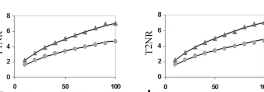
The best use of exam time was more thoroughly ad-dressed in the second series of simulations. In both theT1 andT2cases (Fig. 4a,b), multiple averaging of dual-angle data provides greater precision per unit scan time than single average, multiple flip angle data. Fitting an expo-nential curve to theT1NRvalues of interest, the effects of both increased flip angles and increased averages are char-acterized by:
T1NR兩NimagesfNfa ⫽T1NR2images⫻共Nimages/2兲0.44 [17]
T1NR兩NimagesNav ⫽T1NR2images⫻共Nimages/2兲0.5 [18]
FIG. 3. SimulatedT1NR values calculated over a range ofT1values
calculated from data acquired with the standard set of angles (cir-cle), tuned angles (star), ideal angles (square), and the ideal angles average 5 times (triangle). Maximum precision is achieved through averaging the ideal angle data.
FIG. 4. a:SimulatedT1precision vs. Number of data points collected.b:SimulatedT2precision vs. Number of data points collected.
Precision vs. the number of tuned flip angles sampled is shown by the circular points and follows the relationship described by Eqs. [17] and [19]. Precision vs. the number of averages is shown by the triangular points and follows the relationship described by Eqs. [18] and [20]. For bothT1andT2it is clear that averaging produces the greater precision for any number of total images collected.
whereT1NR兩|NfaandT1NR兩|Navare the precision values associated with multiple flip angles and multiple averages, respectively. From these curves, it is clear that for any number of acquisitions averaging the ideal dual-angle data provides greaterT1precision.
Similarly,T2NRvs.NfaandNav(Fig. 4b) can be mod-eled with analogous functions:
T2NR兩NimagesNfa ⫽T2NR2images⫻共Nimages/2兲0.44 [19]
T2NR兩NimagesNav ⫽T2NR2images⫻共Nimages/2兲0.5. [20]
As in theT1case, it is clear that increasing the number of averages of the ideal dual-angle data provides better T2 precision than increasing the number of individual points along the regression line.
The above equations and figures clearly illustrate the advantage of averaging the dual-angle data. However, since we are not limited to either just averaging or sam-pling individual points, but rather have a variety of possi-ble flip angle and averaging combinations availapossi-ble to us, it is advantageous to derive an expression for any case. Combining Eqs. [17] and [18] and Eqs. [19] and [20] pro-vides the analytical expression for the resultingT1NRor T2NRfor any arbitrary flip angle and averaging combina-tion:
T1or2NRNfa⫽T1or2NR2images⫻共Nfa/2兲0.44
⫻共Nimages/Nfa兲0.5. [21] In an additional simulation that examinedT1NRNfafor a
variety of flip angle and averaging combinations, we con-firmed that precision is maximized through averaging. Set-ting an acquisition limit of 100 in which the data from 2 angles could be averaged 50 times, etc., we calculated
T1NRand compared the simulation results with our pro-posed model. The model closely follows the simulation data and confirms that averaging is the most efficient use of exam time.
We also examined the precision inT2over a range ofT1 andT2values, with and without error included in theT1 measurement. The results of this simulation reveal the SSFP method has maximum precision in the low-to-mid-rangeT1andT2(400 –2000 ms and 20 –100 ms, respectively), which encompasses most brain tissues (with the exception of CSF). When 10% error is included in theT1estimate the average precision across the range of T1 and T2 values decreases 6%, but still performs well over low to midT1 andT2range.
Experimental Results
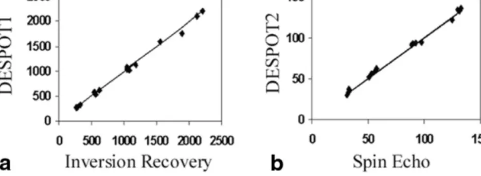
A summary of the phantomT1measurements is shown in Fig. 5a and demonstrates the close agreement between the DESPOT1 and IR values. Analysis of variance (ANOVA) carried out between the sets of data yields a P value of 0.47, confirming that no statistical difference exists be-tween the groups. This agreement is also demonstrated by the low mean percent difference (3.4%) between the groups.
PhantomT2measurements are summarized in Fig. 5b. The calculated P value between the DESPOT2 and SE values of 0.49 indicates that the two approaches are equiv-alent. Once again, the mean percent difference between the groups also demonstrates the close agreement of the two approaches with a 5.6% difference between SE and DESPOT2.
Table 1 contains a summary of brainT1andT2values along with reference IR, SE, and literature values (23–25). As with the phantom data, strong agreement exists be-tween the DESPOT1 or DESPOT2 values and the reference
FIG. 5. a:Comparison ofT1values (ms)
calcu-lated from IR data and DESPOT1 data.b: Com-parison ofT2values (ms) calculated using SE
and DESPOT2 data. In both cases, the points represent average values from a region of inter-est within each tube of the phantom and the solid line represents the line of unity. Close agreement is observed in both the T1and T2
cases.
Table 1
T1andT2Values for Six Common Brain Tissues Calculated Using IR, SE, and SPGR/SSFP With the Ideal Angles
Tissue T1 T2 IR DESPOT1 SE DESPOT2 Gray matter 1002 [56] 1060 [133] 92.1 [2.6] 97.5 [7.3] White matter 615 [12] 621 [61] 69.4 [1.5] 58.1 [4.1] Thalamus 818 [18] 780 [55] 72.7 [1.6] 72.1 [4.3] Putamen 1054 [27] 1014 [101] 71.6 [1.5] 74.1 [4.6] Globus pallidus 780 [18] 726 [53] 54.6 [2.2] 54.7 [7.2] Caudate nucleus 1068 [32] 1112 [132] 79.4 [1.9] 86.7 [6.7]
values, with mean absolute differences of: DESPOT1-IR⫽ 7.1%, DESPOT1-literature⫽6.4%, DESPOT2-SE⫽5.9% and DESPOT2-literature⫽10.6%.
Although the precision of the DESPOT1 values is 3 times worse than the precision observed in the IR results, from Eq. [26] we would expect that equivalent precision could be obtained with DESPOT1 by increasing the SNR of the SGPR images by a factor of 3. The resulting scan time of 16 min represents a significant decrease in imaging time compared with the 75 min required by the 8-point IR technique.
The lower precision of the DESPOT2 measurements (compared with SE) could also be remedied with a similar approach resulting in a total DESPOT1 and DESPOT2 ex-periment time of just 32 min.
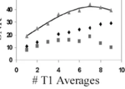
Previously, we theoretically predicted that by using a 75:25 split for theT1:T2portions of the exam time, maxi-mumT1NR⫹T2NRwould be achieved. To experimentally validate this, we performed an experiment in which the T1:T2portions of the exam time were divided as follows: 9:1, 8:2, 7:3, 6:4, 5:5, 4:6, 3:7, 2:8, and 1:9. The results of this experiment (Fig. 6) confirm our theoretical prediction. Fitting a polynomial to this curve and solving for the maximum shows the ideal ratio to be 73:27, which closely matches our theoretical prediction.
Reproducibility of theT1andT2results, determined by calculating the percent SD of a white matter region of interest from four independent experiments, was 6.5% and 5.5% respectively.
Comparison Results
Comparison of the combined DESPOT1 and DESPOT2 ap-proach with conventional and accelerated mapping strat-egies is summarized in Fig. 7 with representative images shown in Fig. 8. The results of these comparisons reveal that our approach has greater efficiency than alternative mapping methods, with the optimized DESPOT1 and DESPOT2 methods showing relative efficiencies of 3.3 (normalized to 8-point IR) and 2.65 (normalized to 7-point SE), respectively.
Unlike Crawley and Henkelman (22), who first deter-mined the optimum experimental parameters for each se-quence (i.e., number ofTIdata points collected, etc.), in our analysis we simply collected the data in a typical
manner. This may not have optimized the precision achieved or minimized the required scan time for each strategy. Thus, the value of efficiency may be underesti-mated in some cases. In the case of IR and SR, Crawley and Henkelman showed maximum efficiency is achieved by sampling at just fiveTIpoints along the recovery curve. Taking this decrease in imaging time into account in-creases the efficiency of these methods by 20% and 16%, respectively. However, DESPOT1 would still outperform both methods by factors of 2 and 1.5, respectively.
With the FSE-IR sequence, using anETLof 4 decreases Tseq by a similar factor. Optimistically, assuming T1NR will not decrease significantly, we would expect this se-quence to have a relative efficiency of 2 compared to IR. Experimentally, this parameter was 2.04. While it is rea-sonable to assume that increasing theETLto 8 or 16 would further increase the efficiency of this sequence, increases inETLresult in undesirable accuracy decreases due toT2 decay effects along the echo train.
Likewise, increasing theETLin the FSE sequence may have further increased its efficiency value. Unfortunately, the signal loss and edge blurring associated with these high ETL values also leads to undesirable decreases in accuracy as well as image degradation.
DESPOT1 and DESPOT2 are also shown to provide su-perior efficiency compared to the alternative accelerated T1mapping strategies of SNAPSHOT FLASH, Look-Locker and accelerated Look-Locker, andT2strategies ofT2FARM and SNAPSHOT FLASH.
DISCUSSION
The experimental and numerical simulation findings pre-sented in the previous sections confirm our hypothesis that the DESPOT1/DESPOT2 approach is an accurate, pre-cise, and high-speed method for combinedT1andT2 map-ping. The approach permits measurement ofT1andT2in a 3D volume (256⫻256⫻100) matrix in less than 13 min with less than 7% error in bothT1andT2(compared with reference IR and SE values) for T1 between 300 and 2000 ms andT2between 30 and 150 ms.
While we have presented concise analytical expressions for the ideal SPGR and SSFP angles, they require a priori
FIG. 7. Bar graphs comparing the relative efficiencies of (a) DES-POT1 and (b) DESPOT2 with alternativeT1andT2mapping
meth-ods, respectively. FIG. 6. T1NR(diamond),T2NR(square),T1NR⫹T2NR(triangle), and
the line fit to T1NR ⫹ T2NR calculated from various exam time
combinations. The total number of images was held constant while the number ofT1andT2images collected was varied. Maximum T1NR⫹T2NRoccurred with sevenT1map averages and threeT2
knowledge of the T1 and T2 ranges present within the imaged object. This does not present a problem in our application, where approximateT1andT2values for brain tissue are widely available. However, in instances where these values are not known, roughT1andT2ranges can be calculated from a set of evenly spaced angles with low resolution over a limited volume. The ideal angles can then be calculated from these approximate ranges. The rapid acquisition and calculation time associated with the presented method allows for this two-step approach with-out requiring excessively long scan times.
The dominant source of error in the accuracy of the DESPOT1 and DESPOT2T1andT2estimates is imprecise knowledge of the flip angles used. Errors in the flip angle arise from two main sources:B1field inhomogeneities and slice profile errors. The 3D nature of the sequence de-creases the magnitude of slice profile errors within the center portion of the 3D slab, particularly when combined with optimized RF pulse designs (e.g., SLR pulses (26)). Unfortunately, errors due to patient-induced B1 inhomo-geneities are more difficult to correct. Variations inB1may occur due to either RF coil nonuniformities or RF attenu-ation and dielectric resonance effects, particularly at very high field. In our neuroimaging application at 1.5 T, this does not appear to present a significant source of error, given the agreement between our results and the literature, especially towards the center of the brain and the basal ganglia — areas associated with absolute changes inT1or
T2 in disease states. In situations where significant B1 inhomogeneities are expected, quantitative B1 mapping could be accomplished as a calibration step, which would then allow for correction of the␣values in our DESPOT1 and DESPOT2 methods. This, however, would increase scan time. Alternatively, B1-insensitive pulses, such as composite pulses or adiabatic fast passage pulses, could be employed. Further work is required to determine the ne-cessity and practicality of these approaches at 1.5 T and higher field strengths.
With several alternative mapping sequences and meth-ods available, the efficiency of each method provides a useful basis for comparison. With an efficiency, relative to IR, of greater than 3, the optimized DESPOT1 method has a higher efficiency than all of the conventional and accel-erated T1mapping techniques examined. Relative to the 7-point SE method, optimized DESPOT2 has a greater efficiency (by a factor of 2.65); furthermore, this efficiency is higher than any of the acceleratedT2mapping methods investigated.
Optimized DESPOT1, with its high efficiency and rapid analysis speed, lends itself to a wide range of imaging applications. For example, fat and blood suppression via inversion nulling techniques use approximate T1values for fat or blood. Inaccuracy in the estimate of theT1value results in suboptimal fat or blood suppression in the final image. Our DESPOT1 method can be used for a fast initial
FIG. 8. AxialT1andT2maps at approximately the same location acquired using (a) IR, (b) FSE-IR, (c) DESPOT1, (d) SE, (e) FSE and (f)
scan to accurately determine T1, thereby improving the performance of these nulling techniques.
The method also provides a simple method for surface coil intensity corrections across an image. Variations in signal intensity across the image, caused by the use of surface coils, will be present in both input images and will therefore be removed by the mapping process. The “flat” T1 map can then be used to produce images with any desiredT1weighting. Combined with a “flat”T2map, an image with any combination ofT1andT2weighting is also easily produced.
Finally, since the combined DESPOT1 and DESPOT2 method provides three quantitative parameter maps (T1, T2, andMo), this method is highly suited to multispectral
segmentation schemes (27,28). Additionally, since theT1, T2, and Momaps could be calculated in real time at the
scanner console, these segmentation/classification schemes could in principle also be performed via the console or in fact in real time during the pulse sequence. This would present radiologists with the ability to analyze and segment data in close to real time, or possibly even adapt pulse sequence changes based on segmentation and classification of tissues/ organs during signal acquisition. Although some of these capabilities have been available previously using nonquan-titative T1- or T2-“weighted” images, we expect that their performance will be greatly enhanced when performed using absoluteT1andT2maps.
CONCLUSION
Our approach of combining DESPOT1 and DESPOT2 per-mits rapid and precise measurement of both T1 and T2 within a clinically acceptable period of time (⬍15 min) for a large volume (25⫻25⫻10 cm) with high resolution (⬍1 mm3voxels). With a mean error of less than 7% in bothT
1 and T2and a reproducibility of 6.4% and 5.5%, respec-tively, the method is comparable to the more conventional approaches, all of which require substantially longer scan times. Additionally, postprocessing time is minimal, re-quiring less than 1 min for both volumes on a 1 GHz PIII PC.
We conclude that the optimized DESPOT1 and DES-POT2 combination approach allows for fully 3D volumet-ric combinedT1andT2mapping of the brain, in a clinical setting, for the first time and makes the generation of real-timeT1andT2maps a reality.
ACKNOWLEDGMENTS
We thank James Odegaard and Glencora Borradaile for assistance in phantom preparation and data collection.
APPENDIX A S⫽f⫻S␣E [A1] sin共␣兲 1⫺E1cos共␣兲⫽ f⫻sin共␣E兲 1⫺E1cos共␣E兲 [A2]
making use of the identities:
cos共␣E兲⫽E1 and sin共␣E兲⫽
冑
1⫺E12 gives: sin共␣兲共1⫺E1 2兲⫽f冑
1⫺E 1 2共1⫺E 1cos共␣兲兲 [A3] squaring both sides and expanding:共1⫺cos2共␣兲兲共1⫺E 1 2兲2 ⫽f2共1⫺E 1 2兲共1⫺2E
1cos共␣兲⫹E12cos2共␣兲兲 [A4] dividing through by and rearranging:
共1⫺E1 2兲⫺共1⫺E 1 2兲cos2共␣兲⫽f2⫺2f2E 1cos共␣兲 [A5] 0⫽f2⫺共1⫺E 1 2兲⫺2f2E 1cos共␣兲⫹共f2E12⫹1⫺E12兲cos2共␣兲 [A6] using the quadratic formula:
cos共␣兲⫽f 2E 1⫾
冑
⫺f2共1⫺E21兲2⫹共1⫺E12兲2 f2E 1 2⫹1⫺E 12 [A7] therefore: ␣⫽cos⫺2冉
f 2E 1⫾共1⫺E1 2冑
1⫺f2 1⫺E12共1⫺f2兲冊
. [A8] APPENDIX B S⫽f⫻S␣E [A9] 共1⫺E1兲sin共␣兲 1⫺E1E2⫺共E1⫺E2兲cos共␣兲⫽ f⫻共1⫺E1兲sin共␣E兲 1⫺E1E2⫺共E1⫺E2兲cos共␣E兲 [A10] making use of the identities:cos共␣E兲⫽⌿ and sin共␣E兲⫽
冑
(1⫺⌿2)where:
⌿⫽共E1⫺E2兲/共1⫺E1E2兲 [A11]
squaring both sides: sin2共␣兲共1⫺E
1E2⫺共E1⫺E2兲⌿兲2
⫽f2共1⫺⌿2兲2共1⫺E
expanding and collecting like terms: cos2共␣兲关2E 1E2⫹E1E2⌿⫺2E1E2共E1⫺E2兲⌿⫹E12E22 ⫹共E1⫺E2兲2⌿2⫺f2共1⫺⌿兲共E1⫺E2兲2兴 ⫹cos共␣兲关2f2共1⫺⌿兲共E 1⫺E2兲⫺2f2共1⫺⌿兲E12共E1⫺E2兲兴 ⫹共1⫺2E1E2⫺2共E1⫺E2兲⌿⫹2E1E2共E1⫺E2兲⌿ ⫹E12E22⫹共E1⫺E2兲2⌿2⫺f2共1⫺⌿兲 ⫹2f2共1⫺⌿兲E 1E2⫺f2共1⫺⌿兲E12E22兲⫽0. [A13] Thus setting: A⫽2E1E2⫹2E1E2⌿⫺2E1E2共E1⫺E2兲⌿⫹E12E22 ⫹共E1⫺E2兲2⌿2⫺f2共1⫺⌿兲共E1⫺E2兲2 [A14] B⫽2f2共1⫺⌿兲共E 1⫺E2兲⫺2f2共1⫺⌿兲E1E2共E1⫺E2兲 [A15] C⫽1⫺2E1E2⫺2共E1⫺E2兲⌿⫹2E1E2共E1⫺E2兲⌿ ⫹E12E22⫹共E1⫺E2兲2⌿2⫺f2共1⫺⌿兲 ⫹2f2共1⫺⌿兲E 1E2⫺f2共1⫺⌿兲E12E22 [A16] allows for the solution using the quadratic equation:
␣⫽cos⫺1共共⫺B⫾
冑
B2⫺4AC兲/2A兲. [A17]APPENDIX C
Following the laws for propagation of error, we are able to examine the impact of error in the measured DESPOT1 signal intensities on theT1estimate. Starting from Eq. [3a] we obtain an expression for the error in theT1(dT1) as:
␦T1 T1 ⫽ ␦m m ⫻ 1 ln共m兲 [A18]
assuming we use the ideal angles whereS␣1⫽S␣2⫽S:
␦T1 T1 ⫽
␦S S ⫻
冑
tan2␣
1⫹tan2␣2⫺0.5 tan␣1tan␣2 tan2␣ 1⫹tan2␣2 ⫻ 1 ln共m兲 [A19] ␦T1 T1 ⫽ ␦S S ⫻ 1 G1 . [A20]
Rewriting Eq. [A20] in terms of image SNR and introduc-ing the new term T1NR (T1-to-Noise Ratio), which pro-vides a measure of the T1 precision as the average T1 divided by the standard deviation, we obtain the final expression:
T1NR⫽SNR⫻G1. [A21]
In a similar manner, we can determine the uncertainty in T2. Starting with Eq. [6a] and letting:
a⫽共m⫺E1兲/共mE1⫺1兲 [A22] and assuming we use the ideal angles whereS␣1⫽S␣2⫽
S,we obtain the expression:
␦T2 T2 ⫽
冑
␦S2 S2 共A⫹B兲⫹␦T12共C⫹D兲⫻ 1 ln共a兲 [A23] with: A⫽ m 2 共m⫺E1兲2冉
tan2␣1⫹tan2␣2⫺0.5 tan␣1tan␣2 tan2␣
1⫹tan2␣2
⫹sin
2␣
1⫹sin2␣2⫺0.5 sin␣1sin␣2 sin2␣ 1⫹sin2␣2
冊
[A24a] B⫽共E12⫻TR2兲/共T14⫻共m⫺E1兲2兲. [A24b] C⫽ m 2E 1 2 共mE1⫺1兲2冉
tan2␣1⫹tan2␣2⫺0.5 tan␣1tan␣2 tan2␣
1⫹tan2␣2
⫹sin
2␣
1⫹sin2␣2⫺0.5 sin␣1sin␣2 sin2␣ 1⫹sin2␣2
冊
[A24c] D⫽共m2⫻E 1 2⫻TR2兲/共T 1 4⫻共mE 1⫺1兲2兲. [A24d] WhenT1is large (⬎100 ms),C⫹D⬇0, so we can simplify Eq. [A23] to:␦T2 T2 ⫽ ␦S S ⫻ 1 G2 , [A25]
which we can rewrite in terms of image SNR and T2NR (T2-to-Noise Ratio) as:
T2NR⫽SNR⫻G2. [A26]
REFERENCES
1. Detre JA, Leigh JS, Williams DS, Koretsky AP. Perfusion imaging. Magn Reson Med 1992;23:37– 45.
2. Gowland P, Mansfield P, Bullock P, Stehling M, Worthington B, Firth J. Dynamic studies of gadolinium uptakes in brain tumours using inver-sion recovery echo-planar imaging. Magn Reson Med 1992;26:241–258. 3. Pitkamen A, Laakso M, Kalviamen R, Partanen K, Vainio P, Lehtovitra M, Riekkinen P, Soininen H. Severity of hippocampal atrophy corre-lates with the prolongation of MRI T2relaxation time in temporal lope epilepsy but not in Alzheimer’s disease. Neurology 1996;46:172–1730. 4. Vymazal J, Righini A, Brooks RA, Canesi M, Mariani C, Leonardi M, Pezzoli G. T1and T2in the brain of healthy subjects, patients with Parkinson’s disease, and patients with multiple system atrophy: rela-tion to iron content. Radiology 1999;211:489 – 495.
5. Bluml S, Schad LR, Boris S, Lorenz WJ. Spin-lattice relaxation time measurement by means of a TurboFLASH technique. Magn Reson Med 1993;30:289 –295.
6. Brix G, Schad LR, Deimling M, Lorenz WJ. Fast and precise T1imaging using a TOMROP sequence. Magn Reson Imag 1990;8:351–356. 7. Henderson E, McKinnon G, Lee TY, Rutt BK. A fast 3D Look-Locker
method for volumetric T1mapping. Magn Reson Imag 1999;17:1163– 1171.
8. McKenzie CA, Chen Z, Drost DJ, Prato FS. Fast acqusition of quantita-tiveT2Maps. Magn Reson Med 1999;41:208 –212.
9. Deichmann R, Adolf H, Noth U, Morrissey S, Schwarzbauer C, Haase A. Fast T2-mapping with SNAPSHOT FLASH imaging. Magn Reson Imag 1995;13:633– 639.
10. Christensen KA, Grand DM, Schulman EM, Walling C. Optimal deter-mination of relaxation times of Fourier transform nuclear magnetic resonance. Determination of spin-lattice relaxation times in chemically polarized species. J Phys Chem 1974;78:1971–1977.
11. Homer J, Beevers MS. Driven-equilibrium single-pulse observation of T1relaxation. A re-evaluation of a rapid ’new’ method for determining NMR spin-lattice relaxation times. J Magn Reson 1985;63:287–297. 12. Homer J, Roberts JK. Conditions for the driven equilibrium single pulse
observation of spin-lattice relaxation times. J Magn Reson 1987;74: 424 – 432.
13. Wang HZ, Riederer SJ, Lee JN. Optimizing the precision inT1 relax-ation estimrelax-ation using limited flip angles. Magn Reson Med 1987;5: 399 – 416.
14. Homer J, Roberts JK. Routine evaluation of Moratios and T1values from driven equilibrium NMR spectra. J Magn Reson 1990;87:265–272. 15. Carr HY. Steady-state free precession in nuclear magnetic resonance.
Phys Rev 1958;112:1693–1701.
16. Hinshaw WS. Image formation by nuclear magnetic resonance: the sensitive-point method. J Appl Phys 1976;47:3709 –3721.
17. Young IR, Burl M, Bydder GM. Comparative efficiency of different pulse sequences in MR imaging. J Comput Assist Tomogr 1986;10:271– 285.
18. Perkins TG, Wehrli FW. CSF signal enhancement in short TR gradient echo images. Magn Reson Imag 1986;4:465– 467.
19. Hendrick RE, Kneeland JB, Stark DD. Maximizing signal-to-noise and contrast-to-noise ratios in FLASH imaging. Magn Reson Imag 1987;5: 117–127.
20. Hawkes RC, Patx S. Rapid Fourier imaging using steady-state free precession. Magn Reson Med 1987;4:9 –23.
21. Buxton RB, Fisel CR, Chien D, Brady TJ. Signal intensity in fast NMR imaging with short repetition times. J Magn Reson 1989;83:576 –585. 22. Crawley AP, Henkelman RM. A comparison of one shot and recovery.
Methods inT1imaging. Magn Reson Med 1988;7:23–34.
23. Vymazal J, Righini A, Brooks RA, Canesi M, Mariani C, Leonardi M, Pezzoli G. T1and T2in the brain of healthy subjects, patients with Parkinson disease, and patients with multiple system atrophy: relation to iron content. Radiology 1999;211:489 – 495.
24. Breger RK, Rimm AA, Fisher ME, Papke RA, Haughton VM. T1and T2 measurements on a 1.5 T commercial MR imager. Radiology 1989;171: 283–276.
25. Steen RG, Gronemeyer SA, Kingsley PB, Reddick WE, Langston JS, Taylor JS. Precise and accurate measurement of proton T1in human brain in vivo: validation and preliminary clinical application. J Magn Reson Imag 1994;4:681– 694.
26. Pauly P, Le Roux P, Nishimura D, Macovski A. Parameter relations for the Shinnar–Le Roux selective excitation pulse design algorithm. IEEE Trans Med Imag 1991;10:53– 65.
27. Mitchell JR, Rutt BK. Improved contrast in multi-spectral phase images derived from MR exams of MS patients. Med Phys 2002;29:727–725. 28. Deoni SCL, Rutt BK, Peters TM. An alternative method for visualizing
m-dimensional MRI data. In: Proc 9th Annual Meeting ISMRM, Glas-gow, 2001. p 784.