A Variance Decomposition for Stock Returns

(1)

?4BER WORKING PAPER SERIES

A VARIANCE DECOMPOSITION FOR STOCK RETURNS

John Y. Campbell

Working Paper No. 3246

NATIONAL 81JREAU OF ECONOMIC RESEARCH 1050 Massachusetts Avenue

Cambridge, MA 02138 January 1990

I am grateful to Rob Stambaugh for assistance with the data, to John Ammer for research aseistance, and to Chris Gilbert, Pete Kyle, Masao Ogaki, Robert Shiller, and participants in the 1989 NBER Summer Institute workshop on New Econometric Methods in Financial Markets for helpful comments and discussion. I acknowledge financial support from the National Science Foundation and the Sloan Foundation. This paper is part of NBER's research program in Financial Markets and Monetary Economics. Any opinions expressed are those of the author not those of the National Bureau of Economic Research.

(2)

NBER Working Paper #3246 January 1990

A VARIANCE DECOMPOSITION FOR STOCK EflURNS

ABSTRACT

This paper shows that unexpected stock returns must be associated with changes in expected future dividends or expected future returns A vector autoregressive method is used to break unexpected stock returns into these two components. In U.S. monthly data in 1927-88, one-third of the variance of unexpected returns is attributed to the

variance of changing expected dividends, one-third to the variance of changing expected

returns, and one-third to the covariance of the two components. Changing expected returns have a large effect on stock prices because they are persistent: a 1% innovation in the expected return is associated with a 4 or 5% capital loss. Changes in expected returns are negatively correlated with changes in expected dividends, increasing the

stock market reaction to dividend news. In the period 1952-88, changing expected. returns account for a larger fraction of stock return variation than they do in the period 1927-51.

JohnY. Campbell

London School of Economics Financial Markets Group Houghton Street

London WC2A 2AE England

(3)

1. Introduction.

What moves the stock market? This apparently basic question has stimulated

voluminous research and heated debate. In this paper I propose a simple way to break stock market movements into two components; one which is associated with changes in rational expectations of future returns, and one which is not. I call the former "news

about future returns", and the latter "news about future dividends". My approach

allows for arbitrary correlation between the two components, and this turns out to be important in practice.

My starting-point is a regression of the stock return, measured over a short period such as a month, onto variables known in advance. Numerous papers have shown that such regressions have a modest but statistically reliable degree of explanatory power.' I combine this regression with other regression equations describing the evolution through time of the forecasting variables. The resulting vector autoregressive (VAR) system can be used to calculate the impact that an innovation in the expected return will have on the stock price, holding expected future dividends constant. This impact is the "news

about future returns" component of the unexpected stock return. The "news about

future dividends" component is obtained as a residual.

In U.S. stock market data, I find that the variance of news about future returns,

and the covaria.nce between the two types of news, are always important contributors

to the variance of unexpected stock returns. The data give this result because the

variables which forecast stock returns are persistent, so that an innovation today has implications for expected returns into the distant future. Also shocks to expected future dividends seem to be negatively correlated with shocks to expected future returns, so that there is a positive covariance between the two components of unexpected stock returns.

Another way to express this result is that the overall variance of stock returns is always greater than the variance of news about cash flows. Short-term predictability of returns can increase the variance of unexpected returns to a surprising degree. The findings here suggest that a satisfactory explanation of stock market volatility cannot ignore short-term predictability.2

The approach used here is different from two others which have been popular in the 1A partial list of references is ca.mpbeu (1987), cutle, Poterha, and Summers (1989a), Fama and Flenth (lQssb, 1989), and Keim and 5tasnhaugh (1986).

2Banky and DeLong (1989) and Froot and Obetfeld (1989) are two exampha of recent papers which attempt to explain stock market volatility using modela in which stock returns are unforecastable.

(4)

recent literature. What I will call the contemporaneous regression approach regresses stock returns on contemporaneous innovations to variables which might plausibly affect the stock market (Cutler, Poterba, and Summers 1989b, Roll 1988). This breaks the return into a component which is a reaction to measured news variables, and a residual (sometimes called "noise"). But the reaction to measured news could occur either be-cause traders' expectations of future dividends change, or bebe-cause their expectations of future returns change. The contemporaneous regression approach does not distinguish these possibilities.

The univariate time-series approach studies the autocorrelation function of stock returns (Conrad and Kaul 1988, Cutler, Poterba, and Summers 1989, Fama and French 1988a, IA and MacKinlay 1988, Poterba and Summers 1988). The objective is to de-compose prices into a "transitory" and a component. The movements of the former are associated with changing rational expectations of returns, but the move-ments of the latter are not. The approach postulates an unobserved components model for the stock price, calculates the implications of the model for the autocorrelations of returns, and then uses observed autocorrelations to estimate the model parameters. It is argued that if the observed autocorrelations are all zero, so that ex posi stock returns

are white noise, then this is evidence that expected returns are constant.

A practical problem is that the univariate time series often delivers only weak evidence against the hypothesis that all autocorrelations are zero.3 This is because

one loses power by forecasting returns using only past returns, ignoring all the other

possible information variables. The autocorrelations of ex posi returns can be very small even when expected returns are variable and highly persistent. The reason is

that innovations in expected returns cause movements in er posi returns in the opposite direction; the resulting negative serial correlation in cx post returns tends to offset the positive serial correlation arising from persistent expected returns. In fact, it is possible to construct an example in which expected returns are variable and persistent, but ex posi returns are white noise.4 A related difficulty is that a strong assumption on the covariance of the two components is needed to identify the parameters of the model

3This .tatement holds for papas whim look at lower frequency retums and 1aiw stocks; see ror example Fans sod Frendi (1988a). Poterba and Swnmers (1988). and recent criti%lea by Jegadeesh (1989), Kim, Nelson, and Starts (1989), Richardson (1989), and stock and Richardson (1989). Conrad and Kaul (1988) and Lo and MacKinlay (1988) find strong evidence against white noise returns, but they are looking at high Frequency weekly data and smaller stocks.

tPoteba and Sunimers (1988) claim that "If market and fundamental values diverge, but beymd sonic range the differences are eliminated by speculative forca, then stock prices will revert to their mean. Retona must be negatively serially correlated at some frequetcy if 'trrmneous' market moves are eventually conerted" (pp.27-28). The example given in section 3 belowshowsthat this statement is notgenerallytrue.

(5)

from the autocorrelations of returns. For both these reasons I argue that a multivariate approach is preferable to the exclusive focus on univariate autocorrelations.

This paper is based on the methods of Campbell and Shiller (1988a, 1988b). Those papers decompose the variance of annual stock returns (and log dividend-price ratios)

into components due to forecasts of cash flows and returns. Forecasting equations are estimated for dividend growth rates and log dividend-price ratios, rather than

returns; hut the forecasting system implies forecasts of returns, because the log stock

return can be well approximated by a linear combination of dividend growth rates and log dividend-price ratios. In this paper I forecast returns explicitly and do not

include dividend growth rates in the analysis. This has the advantage that I can work with higher-frequency monthly data without having to deal with seasonals in dividend payments.

The work of Kandel and Stambaugh (1988) is also relevant for this paper. Kandel and Stambaugh examine the long-run implications of a low-order vector autoregression in returns and a set of forecasting variables. They are able to show that the low-order VAR can account for several long-run characteristics of the data, including the high R2 statisticsobtained in long-horizon regressions by Fama and French (1988a). However

Kandel and Stambaugh do not study the impact of expected return movements on

unexpected returns.

Finally, Campbell (1990) is a brief summary of some of the major results given

here.

The organization of the paper is as follows. The next section sets up the basic framework which will be used to calculate the relation between unexpected returns

and movements in expected returns. Section 3 describes and compares the univariate time-series approach and the VAR approach for decomposing the variance of stock returns. Section 4 reports empirical results for monthly U.S. data in the period 1927-88, and section 5 concludes.

(6)

2. Expected Returns and Unexpected Returns.

The basic equation used in this paper relates the unexpected real stock return in. period t + 1 to changes in rational expectations of future dividend growth and future

stock returns. Writing ht+i for the log real return on a stock held from the end of period t to the end of period t + 1, and d1 for the log real dividend paid during

period t + 1, the equation is

—

Ejlzjti = (Egi

—

— —_E1)

>

ht+i+.

(2.1)

Here E1 denotes an expectation formed at the end of period t, and zdenotes_{a 1-period} backward difference. The parameter p is a number a little smaller than one.

Equation (2.1) is best thought of as a consistency condition for expectations. If the unexpected stock return is negative, then either expected future dividend growth must be lower, or expected future stock returns must be higher, or both. To see why, consider an asset with fixed dividends whose price fails. Its dividend yield is now higher; this will increase the asset return unless there is a further capital loss. Capital losses cannot continue forever, so at some point in the future the asset must have higher returns.

The discounting at rate p in equation (2.1) means that an increase in stock returns expected in the distant future is associated with a smaller drop in today's stock price than is an increase in stock returns expected in the near future. To understand why this is, consider the arrival of news that stock returns will be higher ten periods from now. If the path of dividends is fixed, the stock price must drop to allow a rise ten periods from now. Most of the drop occurs today, but for nine periods there are smaller declines which are compensated by a higher dividend yield. These further declines reduce the size of the drop which is required today.

Formally, equation (2.1) follows from the log-linear "dividend-ratio model" of Campbell and Shiller (l988a). This model is an appropriate framework because it

allows both expected returns and expected future cash flows to affect asset prices. The model is derived by taking a first-order Taylor approximation of the equation relating

(7)

the log stock return to log stock prices and dividends. The approximate equation is

solved forward, imposing a terminal condition that the log dividend-price ratio does not follow an explosive process. Further details are given in the Appendix.

It will be convenient to simplify the notation in equation (2d). Let us define vhj+1 to be the unexpected component of the stock return hg+j:

Let us define qdt+1 to be the term in equation (2.1) which represents news about cash

flows:

'ld,t+l

(E1

—

Letus define to be the term in equation (2.1) which represents news about future

returns:

'ih,t+i

Thenequation (2.1) can be rewritten as

Vh,f+1

=

'ld,t-fl — qh,t+1 (2.2)

2.1. A univariate AR(1) for the expected return.

A useful special case is that in which the expected stock return follows a univariate first-order autoregressive, or AR(1), process.5 Let us define uj+1 to be the innovation

at time t + 1 in the one-period-ahead expected return: (Ej+i —_E)hj+2.

I

the expected return follows a univariate time series process, then 'Th,t+i is an exact function of ug+1. The AR(1) case is

= Eghg+i + ug',

(2.3)

which implies

51t is important to note that thi. process does not restrict the size of the markets information set. In particular, there is no presumption that the relevant information set contains only thehistoryof past asset retrrns. It is quite possible that a very large number of vsrislts isusefulin forecafling the wet return over the nest period the univariate AR(1) assumption merely restricts the way in which the next period's forecsst is related to past foreasts. See Littennan and Weiss (1985) for discussion of the Aft(s) model applied to the expected real return on short d.bt

(8)

'lh,t+i =

— (2.4)

Since p is a number very close to one, this equation says that a i% increase in the

expected return today is associated with a capital loss of about 2% if the AR coefficient is 0.5, a loss of about 4% if the AR coefficient is 0.75, and a loss of about 10% if the AR coefficient is 0.9. Poterba and Summers (1988, Appendix) give a similar result.

Equation (2-4) can also be used to calculate the ratio of the variance of news about future returns to the overall variance of unexpected returns, If the AR(1) model holds, this ratio satisfies

________

— 1

_ci2

p '\2

( fl2

Var[vhj+1] —

— )

—_pci) _{ki — ft2}

(i+f ft2

1ci)k1_ft2)'

(2.5)

where ft2 is the fraction of the variance of stock returns which is predictable. If 2 is 0.025, then the share of news about future expected returns in the variance

of unexpected returns is 0.08 for ci = 0.5,

0.18 for =

0.75, and a startling 0.49 for ci

=

0.9. These parameters are not unreasonable ones for monthly stock returns. An ft2

of 0.025 is quite modest, and a process with =0.9has a half-life of only a little more than six months. This example shows that movements in expected returns can be very important in explaining stock price volatility, even if the predictable component of the monthly stock return is small.

2.2. Real returns and excess returns.

The discussion so far has been couched in terms of real stock returns. For many

purposes it is more natural to work with excess stock returns over some short-term interest rate. If the log real interest rate is rg, then the excess return is just

(9)

— rt+l. _(2.6)

Since eg is Just the difference between two continuously compounded real returns,

the price deflator cancels and it can equally well be measured as the difference between two log nominal returns.

It is straightforward to combine (2.6) and (2.1) to obtain

egi —

= (Eg+i

—

—(Eg+i—

Eg)et+i+j,

(2.7)

or in more compact notation,

Ve,L4.1 = _'ld,t-j-I —

'lr,t+l —

If

the first two terms on the right hand side of (2.8) are treated as a composite residual, then (2.8) has exactly the same form as (2.2). Alternatively, one can work with the three-way decomposition of excess returns given on the right hand side of

(2.8).

(10)

—7--3. Alternative Approaches to Variance Decomposition.

One way to decompose the variance of stock returns is to examine the serial corre-lation of returns. I have called this the imivariate time series approach. For example, if the expected real return follows the AR(1) process given in equation (2.3), then the

ex post return follows an ARMA(1,1) process whose i'th autocovariance is:

Cov(hj+i, ht+i_1) =

c'_'

[covnzu —

(

—

1

..2) var(u)I.

(3.1)

The autocovariances of ex posi returns are all of the same sign and die off at rate 4,; this is a property of the AR.MA(1,l) which is emphasized by Poterba and Summers (1988) and Cutler, Poterba arid Summers (1989a).

Equation (3.1) reveals two difficulties with the univariate time series approach.

First, if the autocova.riances are not all zero then they identify 4, and the term in square brackets in (3.1); but this is not generally enough to identify the innovation

variance of expected returns, Var(u). For that one must make some assumption about the covariance Cov(q, u) between news about future dividends and shocks to expected returns. The assumption generally made is that the covariance is zero. But this is an arbitrary assumption, and I present evidence below that it is false.

Secondly, it is possible that all the autocovariances of stock returns are zero, even

when expected returns are variable and persistent. In this case the univariate time

series approach breaks down completely. The condition for this is

(p

__

CovOld,u)

=

ki—# — 1_4,2)Var(u).

Equation (3.2) can be satisfied with zero covariance Cov(r,d, u) between shocks to cash flows and shocks to expected returns, if the expected return follows a highly persistent process such that 4,= p. Alternatively, it can be satisfied with a positive covariance

between shocks to cash flows and shocks to expected returns, and a less persistent

expected return process which has 4, C p.

Of course, in practice it is unlikely that (3.2) will hold exactly. In the empirical

work in the next section, I estimate the covariance between cash flow and expected —8—

(11)

return shocks to be negative in the U.S. stock market in 1927-88, so that one should find a predominance of negative autocorrelations in stock returns. But these

autocor-relations are all small relative to their standard errors, which makes it hard for the

uriivariate time series approach to give very definite results.

3.1. The VAR approach.

Instead of focusing exclusively on the autocovariances of stock returns, I model the stock return as one element of a vector autoregression. 1 begin by working with real stock returns, and then modify the model to handle excess stock returns.

First, I define a vector tiI which has k elements, the first of which is the real stock return hg+i. The other elements are other variables which are known to the market by the end of period it + 1. Then I assume that the vector zg.,.1 follows a first-order VAR:

=

_Azj _{+ wg+1.} _(3.3)

The assumption that the VAR is first-order is not restrictive, since a higher-order VAR can always be stacked into first-order (companion) form in the manner discussed by Campbell and Shiller (1988a). The matrix A is known as the companion matrix of the

VAR.

Next I define a k-element vector el, whose first element is 1 and whose other elements are all 0. This vector picks out the real stock return hj+t from the vector zj+1: hg+i =

el'zt+i, and vht+1 =

el'wi+t. The first-order VAR generates simple multi-period forecasts of future returns:

=

eltA3+lzg. (3.4)

It follows that the discounted sum of revisions in forecast returns can he written as

(12)

—9--'lh,t+I (Ej+i—Et)EpJht+i+j =

el'EPIA'wg+i

=

ei'pA(I

—

= A'wj+i,

(3.5)

where A' is defined to equal ei'pA(I —

pA)1,

a nonlinear function of the VAR coeffi-cients.

Since "ht+1isthe first element of wi, ei'wj+i, equations (3.5) and (2.2) imply

that

'7d,t+l

=

(ci'

+ A') wg+l. (3.6)

These expressions can be used to decompose the variance of the unexpected stock

return, vh:+1, into the variance of the news about cash flow, '1d,t+1thevariance of

the news about expected returns, qh,t1anda covariance term.

In the VAR context there is no single measure of the persistence of expected returns. But one natural way to summarize persistence is by the variability of the

innovation in the expected present value of future returns, relative to the variability

of the innovation in the one-period-ahead expected return. Thus I define the VAR

persistence measure P4

— a(?M,j+1)

=

0(A'wt+i)

/ , 3.7

c(ei Awt÷i)

where c(x) denotes the standard deviation of x. Another way to describe the statistic

h

is to say that a typical 1% innovation in the expected return will cause a P4%

capital loss on the stock. In the univariate AR(i) case, P4 would just equal p/(i — orapproximately 11(1 —

Giventhe definitions of A and A and a set of VAR estimates, it is straightfor-ward to estimate the VAR persistence measure P4 and the variance decomposition

(13)

for unexpected stock returns. The calculation of standard errors is a little more dif-ficult. The approach I take is to treat the VAR coefficients, and the elements of

the variance-covariarice matrix of VAR innovations, as parameters to be jointly

es-timated by Generalized Method of Moments (Hansen 1982). The 0MM parameter estimates are numerically identical to standard OLS estimates, but 0MM delivers a

heteroskedasticity-consistent variance-covariance matrix for the entire set of

parame-ters (White 1984). Call the entire set of parameparame-ters 7, and the variance-covariance

matrix V.

Any statistic such as the share of the variance of unexpected returns which is

attributed to news about future expected returns can be written as a nonlinear function

1(7)ofthe parameter vector .ThenI estimate the standard error for the statistic in standard fashion as

The VAR approach can be used to analyze excess stock returns as well as real

returns. In this case the basic equation is (2.8) rather than (2.2). If the first two

terms on the right hand side of (2.8) are treated together, then equations (3.3) to (3.6)

hold with et. replacing ht+i. The components of the excess stock return should be

interpreted as "news about future dividends and real interest rates" and "news about future excess returns".

It is more interesting to treat all the terms on the right hand side of (2.8) separately. The vector zf+1 must then include the excess return as its first element, and the

real interest rate r+1 as its second element. Define e2 to be a k-element vector whose

second element is 1, with all other elements zero. Then "news about future excess returns" is Ve,1+1=_A'wH.l,withA' defined as before. "News about future real interest rates" is qr1+1

=

_p'wf+l,where

=

_e2'pA(I—

pA)1wji

= 14'wt+l,.

(3.8)

where p' is defined as e2'pA(I —

pA)1.

The residual "news about future dividends", is given by

e_This_{procedure I. very similar to that used in Campbell and Shilla- (1955a.b). However c&u and Shiller treated} the varlance-covariance matrix of the variables in the VAR as fixed and computed standard snore allowing only for sampling error in the VAR coefficients. Their procedure can be thought of as giving a standard error for a sample variance decomposition, while the procedore used here give a standard error for s population variaswe decomposition

(14)

I I $

= (ci

+A

+p)wj+i-Separate persistence measures can be defined for the expected real interest rate and the expected excess return. Fbr the real interest rate, the persistence measure is

— _________

r

=

a(e2'Awj+i)'

while the persistence measure for the excess return, P, is given by the formula in

equation (3.7).

(15)

4. Application to the U.S. Stock Market.

For the sake of comparability with previous work, I use a standard data set here. I study the behavior of the value-weighted New York Stock Exchange Index, as reported by the Center for Research in Security Prices (CRSP) at the University of Chicago.7

The data set runs from 1926 to 1988, but I reserve the fIrst year for lags so that my

full sample period is 1927 to 1988. I deflate the nominal return on the index using the Consumer Price Index reported in Ibbotson Associates (1989).

The forecasting variables I use for the stock return are the lagged stock return, the dividend-price ratio, and the "relative bill rate", the difference between a short-term Treasury bill rate and its one-year backward moving average. The lagged stock return is included because the stock return forecasting equation will be one equation of a VAR system. The dividend-price ratio is included, following Campbell and Shifler (1988a, 1988b) and Fama and French (1988b), because it should reflect any changes that may occur in future expected returns.8 The ratio is measured as total dividends paid over the previous year, divided by the current stock price.

The relative bill rate is included because many authors, including Fama and Schw-ert (1977) and Campbell (1987), have noted that the level of short-term interest rates

helps to forecast stock returns. The short-term interest rate itself may be nonstationary over this sample period, so it needs to be stochastically detrended. The subtraction of a one-year moving average is a crude way to do this; the relative bill rate can also be written as a triangular moving average of changes in the short-term interest rate, so it is stationary in levels if the short rate is stationary in differences.9 The short rate used is the one-month Treasury bill rate series from Ibbotson Associates (1989).

One problem which arises when interest rate data are used is that the behavior

of interest rates has changed over time. In particular, the Federal Reserve Board held

interest rates almost constant for much of the period up to 1951, when a Federal

Reserve Board-Teasury Accord allowed rates to move more freely. Accordingly, I spilt

the 1926-88 sample at the end of 1951. This also allows a separate Look at the data

from the period around the Great Depression, which may behave quite differently from the postwar data (Kim, Nelson, and Startz 1989).

7

obtain similar results using the cRSP equal-weighted index. The forecaating variables used here predict returna on large stocks as well as small stocks, so the choice of index is not

critical-To see this, consider theasate version of equation (A.2)inthe Appendix.

5knother recently popular way to detrend the interest rate a to uae the yield spread between interest rates of two differest tnsturities. The relative bill rate has at least as moth forecasting power for stock reIn as the long-short yield spread, whid, is inaignilicant whenitis added totheequaLiona reported below.

(16)

4.1. Basic results for real returns.

Panel A of Table 1 reports the basic first-order VAR which I will use to analyze the persistence of expected returns. The first three columns give the regression coefficients for the stock return forecasting equation, the dividend-price ratio forecasting equation,

and the relative bill rate forecasting equation. Together, these coefficients form the

VAR companion matrix A. ileteroskedasticity-corrected standard errors are reported in parentheses. The remaining columns of the table report the regression 1?2 statistics, the joint significance levels of the VAR forecasting variables, and the significance levels for Chow tests of parameter stability.

The If2 statistic for the stock return equation is only 2.4% over the full sample; the forecasting variables are jointly significant at the 1.8% level, but the lagged stock return and the dividend-price ratio are individually insignificant. The other two equations have If2 of 94% and 45% respectively, since the dividend-price ratio and relative bill rate follow quite persistent processes. There is little evidence of cross-effects between these two variables; each one is quite well modelled as a univariate autoregression. There is some evidence of instability in the VAR system, particularly in the equation describing the relative bill rate.

The top row of Table 2 calculates the implications of the VAR estimates for the variance of unexpected returns. Slightly more than a third of the variance of unexpected returns is attributed to the variance of news about future cash flows, slightly less than

a third is attributed to the variance of news about future returns, and the remainder

is due to the covariance term. The correlation between shocks to expected returns and shocks to cash flow is about —0.5, indicating that good news about fundamental value tends to be associated with declines in expected future returns. This means that stock prices move more in response to cash flow news than they would if expected returns

were constant.'0 Finally, the persistence measure hisa little less than 5, indicating

that a i% innovation in the expected return is associated with a 5% capital loss. This is the same effect as would be given by a univariate AR(1) process for the expected return with a coefficient of just under 0.8.

Panels B and C of Table 1, and the second and third rows of Table 2, report

the same statistics for the subperiods 1927-51 and 1952-88. There is no evidence of parameter instability between the first and second halves of these subperiods.

IS_Campbell_{and Kyle (1988) emphasize a similar finding for annual US- stock market data over the period 1871-1986.}

4.2. Univariate implications.

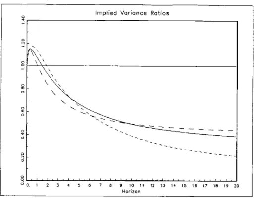
It is of some interest to calculate the univariate time-series implications of the

VAR models estimated in Table i.h1 Figure 1 shows the implied variance ratio statistic of Cochrane (1988) (see also Lo and MacKinlay 1988 and Poterba and Summers 1988). for horizons out to 20 years. These statistics are computed from the VAR estimates in Table 1, and not directly from the data.

The variance ratio statistic V(K) is defined as the ratio of the variance of K-period

returns to the variance of 1-period returns, divided by K. This ratio will be one for

white noise returns; it will exceed one for returns which are predominantly positively autocorrelated, and it will be below one when negative autocorrelations dominate. The ratio can be calculated directly from the autocorrelations of 1-period returns by using

the fact that

V(K) = 1 + 2 :

(i

—

4:) Corr(hj,

h_).

Kandel and Stasnbangh (1PM)report a numberof calculatiom of thi, type.

(18)

Implied variance ratios are shown for the periods 1927-88, 1927-51, and

1952-88. The general pattern is similar in the three periods. The variance ratios rise to a peak between 6 months and 1 year, and then decline steadily The corresponding

implied autocorrelations are positive for the first few months, and then negative; this is what Cutler, Poterba, and Summers (1989a) call the "characteristic autocorrelation function" of stock returns.

The postwar variance ratios differ from the prewar ones in that they rise further

initially, and then decline more slowly. Beyond a horizon of 6 years, however, the

postwar variance ratios lie below the prewar ones. They approach a limit of about 0.2, while the prewar limit is about 0.4. This long-run behavior would of course be almost impossible to detect directly in the data. 12

Fania and French (1988a) characterize the univariate behavior of stock returns in another way. They regress the K-period stock return on the lagged K-period return. The Fama-French regressiqn.coefficient /3(K) is related to the variance ratio statistic

/3(K) =

_____ — 1.

The R2 of the K-period regression is simply the square of /9(K). Figures 2A, 211, and 2C show the implied .112 of Farna-French regressions for horizons out to 20 years. For

comparison, the figures Alto show the implied ,fl2 from regressions of K-period returns on the variables used in the VAR system.

In all cases the ,fl2 statistics rise steeply from their initial values at a 1'month

horizon to a peak at a horizon of several years.13 In the full sample, the Fama-French 112 peaks at about 7% at a horizon of 4 or 5 years, while the VAR 112 peaks at about

13% at a horizon of 3 or 4 years. The prewar peak 112 is 5% for the Fama-French regression and 9% for the VAR regression. In the postwar period, the 112 statistics reach much higher peaks at longer horizons: almost 20% at 9 years for the Fama-French regression, and over 40% at 6 years for the VAR regression. In general the

VAR 112 statistics are about twice as high as the Fama-French 112 statistics, which is 13_Kim,_{Nelson, and Starts (1989) report that reliable direct evidasce of mean revecsinn is bond only in prewar dat&} 13_This_{does not necessarily mean that econometric benefits are obtainable by working with long-horizon returns or} furth lags of the forecasting variabis. In fact, if the VAR(l) model is corremly specified, then no further lags of the VAa variabimare relevantfor forecasting returns once the most recent values have hen included.

(19)

an indication of the benefits obtainable from a multivariate rather than a univariate

approach to stock returns.

4.3. How robust are the results?

The variance decomposition for stock returns is quite robust to changes in VAR

lag length and data frequency. I support this claim in the lower panels of Table 2,

where I give results for a monthly VAR with 6 lags and a quarterly VAR with 4 lags. The 6-lag monthly VAR gives almost the same results as before; the 4-lag quarterly

VAR tends to give greater importance to the variance of news about future returns,

and less importance to the covariance term, but is otherwise quite similar.

The variance decomposition is somewhat more sensitive to changes in the fore-casting variables which are used. The critical variable appears to be the dividend-price

catio When this variable is included in the VAR, the decomposition is much the

same even if the relative bill rate is dropped from the system or replaced by the

long-short yield spread. But when the dividend-price ratio is excluded from the system,

the variance of news about future cash flows is given a more important role while the variance of news about future returns becomes less important and the covariance term is imprecisely estimated.

Fama and Ftench (1990) suggest that the yield spread between low- and

high-quality corporate bonds is a good substitute for the dividend-price ratio in forecasting stock returns. This appears to be true in the prewar period, but in tbe postwar sample the quality yield spread is insignificant for forecasting stock returns when it is added to the relative bill rate. Replacement of the dividend-price ratio by the quality yield spread

causes a 1% reduction in the R2 of the stock return forecasting equation. With this

replacement, the VAR system attributes 1.686 (with a standard error of 0.719) of the variance of unexpected returns to the variance of news about cash flow, 0.649 (0.757) to the variance of news about future returns, and -1.334 (1.465) to the covariance term. These estimates are much less precise than those reported in Table 2.

The variance decomposition can also be sensitive to the imposition of restrictions on the VAR system. For example, if one imposes the restriction that the expected stock return follows a univariate AR(1) process, the restricted expected return is primarily

driven by the relative bill rate, with little weight on the dividend-price ratio. (The

system must use one or the other variable rather than both, because the two variables

(20)

follow different AR(1) processes so no combination of them is well described by an

AR(1) process.) The variance decomposition that results is similar to that obtained

when the dividend-price ratio is dropped from the basic model. The univariate AR( 1)

restriction is not rejected in the prewar data, but is rejected at the 1.8% level in the

postwar period.

A rather different concern about the variance decomposition is that it may be

affected by small-sample bias. To address this concern, I report the results of a Monte Carlo study in Table 3. I use two alternative data generating processes (DOP's), both based on the models estimated in Table 1. The "estimated DGP" simply takes the VAR system from Table 1 and sets the coefficients in the stock return forecasting equation

to zero. Artificial data are generated by drawing standard normal random variables

and feeding them through this system. The resulting data match the moments of the real data quite closely, except that the artificial stock returns are unforecastable and are moved entirely by news about future dividends, so that Var(t)df+1) =_Var(vh,t+1).

The "unit root DGP" adjusts the VAR coefficients from Table 1 in such a way that the dividend-price ratio follows a process with a unit root. The first row of the matrix A is set to zero as before, but also the (2,2) element is set to 1 and the (3,2) 'element is set to zero. This means that the matrix A has a unit eigenvaiue.

The unit root DGP matches the data less well. (Dickey-f'uller tests reject the hypothesis that the dividend-price ratio has a unit root at the 1% level or better in the full samle and both subsaniiples.) The reason to use this DOP is that unit roots

in regressors cause well-known problems with standard statistical methods. The unit root DGP enables me to check whether the results reported above are robust to these types of problems.

The Monte Carlo study examines the small-sample behavior of three statistics from Table 2. The first is the joint significance of the VAR variables for forecasting monthly

stock returns, reported in the first column of Table 2. The second statistic is the ratio of the variance of news about future dividends to the total variance of unexpected stock returns, Var(?)dj+l)/Var(vhj+1), reported in the second column of Table 2. The third

statistic is the significance level in a test of the hypothesis that this ratio equals one

(computed from the standard error reported in the second column of Table 2). Table 3 repeats the results from Table 2, and then gives their empirical significance levels: the fraction of 1000 Monte Carlo runs which generated statistics further from the null

than the ones found in the data. This exercise is done separately for the full sample

(21)

period arid each subsample.

The estimated DCP reveals some finite-sample bias in the results of Table 2. There is only a very small bias in the predictability of one-period stock returns, but the test

that the dividend variance ratio equals one is more seriously biased. Over the full sample, this test had an asymptotic significance level of better than 0.01%, but it

rejected more strongly in the artificial data 1.8% of the time. In the first subsample, the asymptotic significance level is 1.3%, but the empirical significance level is only 17.5%. This bias is important, but it is riot severe enough to change the general flavor of the empirical results.

The bias is greatly magnified when the unit root DGP is used. Over the full sample, the empirical significance level of the test that the dividend variance ratio equals one is a startling 46%, when the asymptotic significance level is less than o.oi%. It is clear that the presence of a unit root in the dividend-price ratio has a devastating effect on the performance of the variance decomposition procedures. Even the unit root DGP, however, is unable to account for the results found in the postwar sample period. Not a single Monte Carlo simulation delivered more predictable stock returns, or dividend

variance ratios further from one, than were found in the actual data. In the 1952-88

period, the evidence for predictable stock returns is overwhelming.

4.4. Results for excess returns.

Table 4 reports a variance decomposition for excess returns, using equations (2.8),

(3.8), and (39). The variance of unexpected excess returns is decomposed into the variance of news about dividends., 'Jdt+l' the variance of news about real interest

rates, qr,t+l, thevariance of news about future excess returns, q6,g+l,andcovariances among these shocks. The VAR system includes the excess return 61+1, the real interest

rate rj÷1,the dividend-price ratio, and the relative bill rate. The first panel reports

results for a 1-lag VAR, while the second panel gives results for a 4-lag VAR.14 In both panels the variance of news about future real interest rates is very small. The covariances between news about real interest rates and news about other variables

are also small. It seems that news about real interest rates cannot account for large

'

Since there are now 4 variableincad, equation, there are roars parameters to be estimated for any given lag length.

A6-lag VAR baa 24 parasnetcein eachequation and 106 parasneterain all, whid, cauaed computational problema.

(22)

movements in stock prices.15 One reason for this is that movements in the expected real rate are much less persistent than movements in the expected reai stock return or the expected excess stock return. The persistence measure F in Table 4 is quite similar to the measure h in Table 2, whereas the persistence measure P for the expected real interest rate is much smaller. In general, the variance decomposition given in Table 4 is similar to that in Table 2.

13_For._{a similar argument that movements in real interest rate differentials do not account for real exchange rate}

move-ments, see Campbell and Garish (1987}.

(23)

5. Conclusion.

In this paper I have argued that expected stock returns change through time in a fairly persistent fashion. The persistence of the expected return process means that

changes in expected returns can cause sizeable capital gains and losses. Using monthly data on the New York Stock Exchange value-weighted index over the period 1927-88, I estimate that a typical 1% increase in the expected return is associated with a capital loss of 4 or 5%.

The variability and persistence of expected stock returns account for a considerable degree of volatility in unexpected returns. I estimate that over the full sample period, the variance of news about future cash flows accounts for only a third to a half of the variance of unexpected stock returns. The remainder of the stock return variance is due to news about future expected returns. It is important to note that news about future returns is not independent of news about cash flows. Increases in future expected cash

flows tend to be associated with decreases in future expected returns, a correlation which amplifies the volatility of stock returns. This finding is very similar to the

"overreaction to fundamentals" reported by Campbell and Kyle (1988).

Similar results obtain in the subperiods 1927-51 and 1952-88. However the impor-tance of expected return variation is greater in the postwar period. This contrasts with the fact that univariate analyses typically show greater evidence of mean reversion in stock prices before World War II.

The results apply almost equally well to real stock returns, and to stock returns

measured in excess of a short-term Treasury bill rate. The variability of news about future excess stock returns is much greater than the variability of news about future

real interest rates, and the latter has only a relatively small impact on stock returns.

The reason for this is that the variables which forecast real interest rates are not highly persistent. This casts doubt on explanations of variation in expected real stock returns which rely primarily on movements in real interest rates.16

Several caveats are worth mentioning. First, the results summarized above are

point estimates with fairly wide confidence intervals. Both asymptotic standard errors

and the results of a small Monte Carlo study show that there is only weak evidence for stock return predictability in the prewar period. The evidence that returns are

predictable is overwhelming only in the period after 1952. '6One recent example is Ceccketti, ham, and Mark (1989).

(24)

Secondly, the results are dependent on a particular specification of the information

set which agents use to forecast stock returns. The variance decompositionalters

considerably if the dividend-price ratio is excluded from the set of forecasting variables.

It does not seem to be much affected by other changes in the information set,in

particular by increases in VAR lag length or changes in the interest rate variablewhich is used.

More generally, if agents have more information than is captured by the VAR, this can affect the variance decomposition given here. Of course, extra information can only increase the 1-period predictability of returns; but it isconceivable that it could decrease the share of return variance which is attributed to news about future

expected returns. This possibility can be ruled out in the special case of a univariate

AR(1) process for the expected return, but this case does not seem to fit

the data

particularly well.

It is also important to note that the variance decomposition of this paper cannot be given an u.na.rnbiguous structural interpretation. Although I have referred to "news about dividends" and 'news about future returns", the results here do not necessarily

mean that there is one-way causality from dividends and expected returns to stock

prices. In general these variables are all determined simultaneously.

The approach of this paper can be developed in several directions. One important

task is to try to find an economic explanation of changing expected returns. This is

of course an immensely active research area. This paper offers persistence as an extra dimension in which theories must fit the data.

Another interesting extension is the application of the VAR systems used here to cross-sectional asset pricing. Intertemporal asset pricing models explain cross-sectional risk premia as arising from the covariances of individual asset returns with the return on invested wealth (the market portfolio) and with news about future returns on invested

wealth.. The VAR structure used here can be a way to give these models increased

empirical content.

(25)

Appendix; The Dividend-Ratio Model

The dividend-ratio model of Campbell and Shiller (1988a) is derived by taking a first-order Taylor approximation of theequationdefining the log stock return, hi =

log(P + Dt+i) —

log(Pj). The resulting approximation is

(A.1)

where h1 and dj have already been defined, öj is the log dividend-price ratio dt —_pt,

and p1 is the log real stock price at the end of period t. The parameter p is the

average ratio of the stock price to the sum of the stock price and the dividend, and the constant k is a nonlinear function of p.17 Equation (A.1) says that the return on

stock is high if the dividend-price ratio is high when the stock is purchased, if dividend growth occurs during the holding period, and if the dividend-price ratio falls during

the holding period.

Equation (A. 1) can be thought of as a difference equation relating 51to

Sj., zdt+i

and hj+i. Solving forward, and imposing the terminal condition that .oM+1 =

0,Campbell and Shiller (1988a) obtain

51

=

Ep.P'{hj+j—Adt+j] —

j4,.

(A.2)

This equation says that the log dividend-price ratio 51canbe written as a

dis-counted value of all future returns and dividend growth rates zdj+5, discounted

at the constant rate p less a constant k/(1 —p). If the dividend-price ratio is high today, this will give high future returns unless dividend growth is low in the future. It is important to note that all the variables in (A.2) are measured er post; (A.2) has been obtained only by the linear approximation of he+i and the imposition of a condition

that 51+doesnot explode as increases.

17_Equation_{(A.l) and the otha fonnidsa given here differ slightly from those in campbell and Shiller (lPSSa, 1958b}}

because the notation here uses a different timing convsflion.Inthis paper I define the time I stock price and conditional expectation of future variablm to he measured at theend ofperiod Cratherthan the beginning of period I. This conforms with the more standanl practice inthefinance literature.

(26)

However (A.2) also holds cx ante. If one takes expectations of equation (A.2), conditional on information available at the end of time period t, the left hand side

is unchanged since 5tisin the information set, and the right hand side becomes an

expected discounted value. Using the cx ante version of (A.2) to substitute fig and 6t-F1 outof (Al), I obtain (2.1).18

In the empirical work in the paper, I use sample means to set p = 0.9962 for monthly data, and p = (0.9962)forquarterly data. The results are not sensitive to

variation in p within a plausible range.

See Campbell and 5hiller (1988a) for an evaluation of the quality of thelinearapproximation in equations(Al)and (A.2).

(27)

Bibliography

Barsky, Robert B. and J. Bradford DeLong, "Why Have Stock Prices Fluctuated?"1 unpublished paper, June 1989.

Campbell, John Y., "Stock Returns and the Term Structure", Journal of Financial Economics 18:373-399, June 1987.

Campbell, John Y., "Measuring the Persistence of Expected Returns", forthcoming

American Economic Review Papers and Proceedings, May 1990.

Campbell, John Y. and Richard H. Clarida, "The Dollar and Real Interest Rates",

Carnegie-Rochester Conference Series on Public Policy 27:103-139, Fall 1987. Campbell, John Y. and Albert S. Kyle, "Smart Money, Noise Trading, and Stock Price

Behavior", NBER Technical Working Paper 71, October 1988.

Campbell, John Y. and Robert J. Shiller (1988a), "The Dividend-Price Ratio and Ex-pectations of Future Dividends and Discount Factors", Review of Financial Studies

1:195-228, Fall 1988.

Campbell, John Y. and Robert 3. Shiller (1988b), "Stock Prices, Earnings, and

Ex-pected Dividends", Journal of Finance 43:661-676, July 1988.

Cecchetti, Stephen C., Pok-sang Lam, and Nelson C. Mark, "Mean ReveSon in Equi-librium Asset Prices", unpublished paper, Ohio State University, 1989.

Conrad, Jennifer and Gautarn Kaul, "Time-Variation in Expected Returns", Journal

of Business 61:409-425, 1988.

Cutler, David M., James M. Poterba, and Lawrence H. Summers (1989a), "Speculative Dynamics", unpublished paper, June 1989.

Cutler, David M., James M. Poterba, and Lawrence H. Summers (198Db), "What Moves Stock Prices?", Journal of Portfolio Management 15:4-12, Spring 1989.

Fama, Eugene F. and Kenneth R. French (1988a), "Permanent and Temporary Com-ponents of Stock Prices", Journal of Political Economy 96:246-273, April 198K

Fkrna, Eugene F. and Kenneth R. Ftench (1988b), "Dividend Yields and Expected

Stock Returns", Journal of Financial Economics 22:3-25, October 1988.

Fame., Eugene F. and Kenneth R. French, "Business Conditions and Expected Returns on Stocks and Bonds", forthcoming, Journal of Financial Economics, 1989. Fama, Eugene F. and G. William Schwert, "Asset Returns and Inflation", Journal of

Financial Economics 5:115-146, 1977.

Froot, Kenneth A. and Maurice Obstfeld, "Intrinsic Bubbles: The Case of Stock

Prices", unpublished paper, June 1989.

Hansen, Lairs Peter, "Large Sample Properties of Generalized Method of Moments

Estimators", Econometrica 50:1029-1054, November 1982.

(28)

Hansen, Lars Peter and Kenneth 3. Singleton, "Stochastic Consumption, Risk Aversion, and the Temporal Behavior of Asset Returns", Journal of Political Economy

91:249-265, April 1983.

Ibbotson Associates, Stocks, Bonds, Bills, and Inflation: 1989 Yearbook, Chicago, 1989. Jegadeesh, Narasimhan, "On Testing for Slowly Decaying Components in Stock Prices", unpublished paper, Anderson Graduate School of Management, UCLA, March 1989.

Kandel, Shmuel and Robert F. Stambaugh, "Modelling Expected Stock Returns for Short and Long Horizons", Working Paper 42-88, Rodney L. White Center for

Financial Research, Wharton School, University of Pennsylvania, 1988.

Keim, Donald B. and Robert F. Stambaugh, "Predicting Returns in the Stock and

Bond Markets", Journal of Financial Economica 17:357-390, December 1986.

Kim, Myung Jig, Charles R. Nelson, and Richard Startz, "Mean Reversion in Stock

Prices? A Reappraisal of the Empirical Evidence", unpublished paper, University of Washington, May 1989.

Litterman, Robert B. and Laurence Weiss, "Money, Real Interest Rates and Output; A Reinterpretation of Postwar U.S. Data", Econometrica 53:129-156, January 1985. Lo, Andrew W. and A. Craig MacKinlay, "Stock Market Prices Do Not Follow Random

Walks: Evidence from a Simple Specification Test", Review of Financial Studies

1:41-66, Spring 1988.

Poterba, James M. and Lawrence H. Summers, "The Persistence of Volatility and Stock Market Fluctuations," American. Economic Review 76:1142-1151, December 1986. Poterba, James M. and Lawrence H. Summers, "Mean Reversion in Stock Prices;

Ev-idence and Implications", Journal of Financial Economics 22:27-59, October 1988. Richardson, Matthew, "Temporary Components of Stock Prices: A Skeptic's View",

unpublished paper, Graduate School of Business, Stanford University, 1989. Roll, Richard, "p2", Journal_{of Finance 43:541-566, July 1988.}

Stock, James H. and Matthew Richardson, "Drawing Inferences from Statistics Based on Multi-Year Asset Returns", unpublished paper, Kennedy School of Government, Harvard University, and Graduate School of Business, Stanford University,

Novem-ber 198t

White, Halbert, Asymptotic Theory for Econometricians, Academic Press; Orlando, Florida, 1984.

(29)

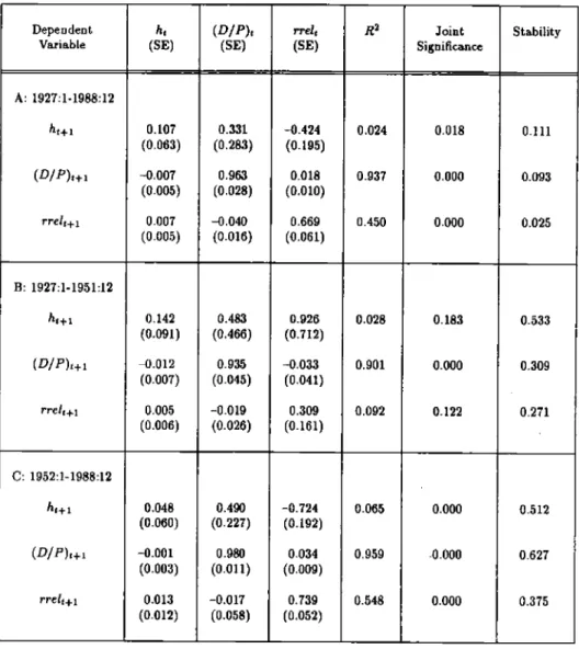
Table 1: Basic VAR flaultsforReal Stock Returns Dependent Variable h1 (SE) (D/P)1 (SE) rrelt (SE) ft2 Joint Significance Stability A: 1927:1-1988:12

h1

(D/P).,.i rre111 0.107 (0.063) —0.007 (0.005) 0.007 (0.005) 0.331 (0.283) 0.963 (0.028) —0.040 (0.016) -0.424 (0.195) 0.018 (0.010) 0.669 (0.061) 0.024 0.937 0.450 0.018 0.000 0.000 0.111 0.093 0.025 B: 1927:1-1951:12 h441 (D/P)1i rret+i 0.142 (0.091) —0.012 (0.007) 0.005 (0.006) 0.483 (0.466) 0.935 (0.045) —0.019 (0.026) 0.926 (0.712) —0.033 (0.041) 0.309 (0.161) 0.028 0.901 0.092 0.183 0.000 0.122 0.533 0.309 0.271 . C: 1952:1-1988:12 h1.,.1 (DIP),.,.1 rrctgi 0.048 (0.060) —0.001 (0.003) 0.013 (0.0 12) 0.490 (0.227) 0.980 (0.011) —0.017 (0.058) —0.724 (0.192) 0.034 (0.009) 0.739 (0.052) 0.065 0.959 0.548 0.000 .0.000 0.000 0.512 0.627 0.375

Notes: h is the log real stock return over a month, (D/P) isthe ratio of total dividends paid over the previous year to the current stock price, and ret is the one-month Treasury bill rate minus a one-year

backward moving average. Standard errors and test statistics are corrected for heteroskedasticity, "Joint

significance" is the significance level for a test of the hypothesis that all regression coefficients are zero.

"Stability" is the significance level for a Chow test that all regression coefficients are the same when the full sample is split at the end of 1952, or when the subsamples are split at their midpoints.

(30)

Tkble 2: Variance Decomposition for Real Stock Returns

VAR Specification

and Time Period .fl (Sig.) Var(q4 (SE) Var(rm) (SE) —2Cov(oo,qe) (SE) Corr(qg,h) (SE) Ph (SE) Is, D/P, reel 1 lag, monthly A: 1921:1-1988:12 B: 1927:1-1951:12 C: 1952:1-1988:12 0.024 (0.018) 0.028 (0.183) 0.065 (0,000) 0.369 (0.119) 0.437 (0.226) 0.127 (0.016) 0.285 (0.145) 0.185 (0.182) 0.772 (0.164) 0.346 (0.046) 0.378 (0.053) 0.101 (0.153) —0.534 (0.127) —0.664 (0.118) —0.161 (0.256) 4.772 (2.247) 3.258 (2.414) 5.794 (1.469) Is, DJP, reel 6 lags, monthly A: 1927:1-1988:12 B: 1927:1-1951:12 C: 1952:1-1988:12 0.081 (0.004) 0.129 (0.083) 0.118 (0.000) 0.538 (0.181) 0.661 (0.363) 0.127 (0.035) 0.265 (0.162) 0.118 (0.142) 0.797 (0.175) 0.197 (0.121) 0.222 (0.288) 0.075 (0.165) —0.261 (0.203) —0.398 (0.565) -0.118 (0.269) 3.972 (2.253) 1.909 (1.515) 4.100 (1.112) Is, D/P, reel 4 lags1 quarterly A: 1927:1-1988:4 B: 1927:1-1951:4 C: 1952:1-1988:4 0.162 (0.045) 0.307 (0.024) 0.213 (0.000) 0.334 (0.096) 0.428 (0195) 0.158 (0.067) 0.497 (0.193) 0.476 (0.166) 0.916 (0.184) 0.170 (0.186) 0.096 (0.236) —0.074 (0.211) —0.208 (0.269) —0.106 (0.290) 0.097 (0.257) 2.726 (1.435) 1.856 (0.820) 7.289 (5.437)

Notes: .R is the fraction of the variance of monthly real stock returns which is forecast by the VAR system,

and 51g. is the joint significance of the VAR forecasting variables. tJd and ' representnews about future

dividends and news about future returns respectively They are calculated from the VAR system using equations (3.6) and (3.5). The three terms Var(tld), Vsr(qs), and —2Cov(rj5,rj) are given as ratios to the variance of the unexpected stock return at,sofrom equation (2.2) they add up to one. The persistence measure Pa is defined in equation (3.7). A typical 1% innovation in the expected real return is associated with a P5% capital loss on the stock.

(31)

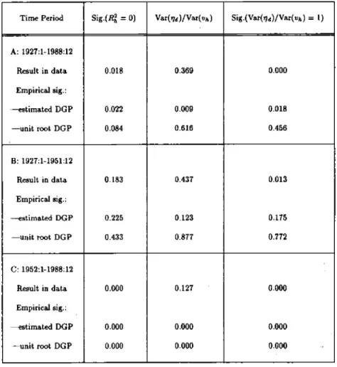
Table 3: Monte Carlo Simulations

Time Period Sig.(R =0) Var(d)/Var(vs) Sig.(Var(i4/Var(vt) =1)

A: 1921:1-1988:12 Result in data Empirical 51g.: —estimated DGP —unit root DGP 0.018 0.022 0.084 0.369 0.009 0.616 0.000 0.018 0.456 B: 1927:1-1951:12 Result in data Empirical sig.: —estimated DGP —unit root DGP 0.183 0.225 0.433 0.437 0.123 0.877 0.013 0.175 0.172 C: 1952:1-1988:12 Result in data Empirical sig.: —estimated DGP —unit root DGP 0.000 0.000 0.000 0.127 0.000 0.000 0.000 0.000 0.000

Notes: This table reports the results of a Monte Carlo experiment. The data generating process was the one estimated in Table 1, setting the coefficients in the return forecasting equation to zero ("estimated DGP") or setting these coefficients to zero, the coefficient of DIP on lagged D/P equal to one, and the coefficient of ritZonlagged D/P equal to zero ("unit root DGP"). Each column of the table reports one statistic from Table 2. The result found in the data is reported, along with the fraction of 1000 runs which rejected the null more strongly than did the data. In the first column, the statistic is the joint significance of the VAR forecasting variables for monthly stock returns. In the second column, the statistic is the estimated share of news about future dividends in the variance of unexpected stock returns. In the third column, the statistic is the significance level for a Wa.ld test of the hypothesis that this share equals one.

(32)

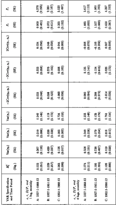
Table 4: Variance Decomposition ('or Excess Stock Returns VAR Specification arid Time Period

R

_(Sig.) Var(qd) (SE) Var(or) (SE) Vsr(eh) (SE) —2Cov(u,e,jr) (SE) —2Cov(qj,ije) (SE) 2Cov(,q.) (SE) Pr _(SE) 1', _(SE) a, r, D/P, red 1 lag, monthly A: 1927:1-1988:12 H: 1927:1-1951:12 C: 1952:1-1988:12 0JD23 _(0.051) 0.029 (0.257) 0.065 (0.000) 0.367 _(0.126) 0.439 _(0.237) 0.126 _(0.017) 0.010 (0.006) 0.020 (0.020) 0.003 (0.002) 0.212 _(0.145) 0.119 _(0.173) 0.734 _(0.153) 11.023 _(0.048) 0.098 (0.122) -0.003 (0.006) 0.323 (0.068) 0.276 (0.163) 0.096 (0.160) 0.034 (0.050) 0.048 (0.050) 0.044 (0.060) 0.909 (0.461) 0.972 (0.611) 0.355 (0.152) 4.376 _(2.295) 2.381 _(2.167) 5.520 _(1.497) a, r, DIP, reel 4 lags, monthly A: 1927:1-1988:12 H: 1927:1-1951:12 C: 1952:1-1988:12 0.074 (0.011) 0.105 (0.293) 0.109 (0.000) 0.508 _(0.191) 0.738 _(0.487) 0.109 _(0.030) 0.049 (0.028) 0.079 (0.054) 0-018 (0.012) 0.233 _(0.148) 0.125 _(0.179) 0.764 _(0.134) 0.080 (0.094) 0.286 (0.272) -0.014 (6.025) 0.135 _(0.141) _-0.124 _(0.615) . 0.036 _(0.172) —0.006 (0.076) —0.106 (0.209) 0.087 (0.096) 1.665 _(0.893) 1.537 _(0.888) 0.6.59 _(0.287) 3.617 _(2.113) 1.960 _(1.763) 4.297 _(1.213) Notes: R is the fraction of the variance of monthly excess stock returns which is forecast hy the VAR system sad Sig. is the joint significance of the VAR forecasting variables. q, ri,, and 'h represent news shout future dividends, future rest interest rates and future excess returns respectively. They are calculated from the VAR system using equations (3.5), (3.8), and (3.9). The terms Var(r), Vsr(qr), Var(q4, 2Cov(;js, Or), 2Cov(qd, O4 and 2Cov(qr, rk) are given as ratios to the variance of the unexpected excess retern v, so from equation (2.8) they add up to one. Pr and P are the persistence inca ares for real rates slid excess returns defined in eqasLions (3.10) siid (3.7) respectively.

(33)

Implied Variance Ratios

Figure 1 Implied Variance Ratios

Solid line, 1927-88; dashed line, 1927-51; short dashed line, 1952-88. Variance ratios are calculated from the VAR(1) models estimated in Table 1.

0

C

00 1

2 3 4 5 6

7 3

9 10 ii 12 13 14 5 16 17 iS 19 20

(34)

Implied R—Squared Statistics

Figure 2A; Implied R2 Statistics, 1927-88

Solid line, R2 from regression of the K-year return on the VAR forecasting variables

used in TaMe 1; dashed line, 112 from regression of the K-year return on the lagged K-year return. K is measured on the horizontal axis. 112 statistics are calculated from the VAR(I) model estimated in Table 1, Panel A.

2 3

4 5 § 7 5 9 10 11 12 13 14 15 5 17 15 lB 20

(35)

Implied R—Squared Statistics

Figure 2B; Implied ft2 Statistics, 1927-51

Solid line, ft2 from regression of the K-year return on the VAR forecasting variables

used in Table 1; dashed line, ft2 from regression of the K-year return on the lagged K-year return. K is measured on the horizontal axis. ft2 statistics are calculated from the VAR(1) model estimated in Table 1, Panel B.

(36)

Implied R—Squcred Statistics

Horizon

Figure 2C: Implied ft2 Statistics, 1952-88

Solid line, ft2 from regression of the K-year return on the VAR forecasting variables

used in Table 1; dashed line, ft2 from regression of the K-year return on the lagged K-year return. K is measured on the horizontal axis. ft2 statistics are cakulated from

the VAR(1) model estimated in Table 1, Panel C.