Kernel Methods for Tree Structured Data

Universit`

a di Bologna, Padova

Ciclo XXI

Settore scientifico disciplinare: INF/01

Kernel Methods for Tree Structured Data

Giovanni Da San Martino

Coordinatore Dottorato: Relatore:

Prof. S. Martini Prof. A. Sperduti

Machine learning comprises a series of techniques for automatic extraction of mean-ingful information from large collections of noisy data. In many real world applica-tions, data is naturally represented in structured form. Since traditional methods in machine learning deal with vectorial information, they require an a priori form of preprocessing. Among all the learning techniques for dealing with structured data, kernel methods are recognized to have a strong theoretical background and to be effective approaches. They do not require an explicit vectorial representation of the data in terms of features, but rely on a measure of similarity between any pair of objects of a domain, the kernel function. Designing fast and good kernel functions is a challenging problem. In the case of tree structured data two issues become relevant: kernel for trees should not be sparse and should be fast to compute. The sparsity problem arises when, given a dataset and a kernel function, most structures of the dataset are completely dissimilar to one another. In those cases the classifier has too few information for making correct predictions on unseen data. In fact, it tends to produce a discriminating function behaving as the nearest neighbour rule. Sparsity is likely to arise for some standard tree kernel functions, such as the subtree and subset tree kernel, when they are applied to datasets with node labels belonging to a large domain. A second drawback of using tree kernels is the time complexity required both in learning and classification phases. Such a complexity can sometimes prevents the kernel application in scenarios involving large amount of data.

the statistical properties of the dataset, thus reducing its sparsity with respect to traditional tree kernel functions. Specifically, we propose to encode the input trees by an algorithm able to project the data onto a lower dimensional space with the property that similar structures are mapped similarly. By building kernel functions on the lower dimensional representation, we are able to perform inexact matchings between different inputs in the original space.

A second contribution is the proposal of a novel kernel function based on the convolution kernel framework. Convolution kernel measures the similarity of two objects in terms of the similarities of their subparts. Most convolution kernels are based on counting the number of shared substructures, partially discarding informa-tion about their posiinforma-tion in the original structure. The kernel funcinforma-tion we propose is, instead, especially focused on this aspect.

A third contribution is devoted at reducing the computational burden related to the calculation of a kernel function between a tree and a forest of trees, which is a typical operation in the classification phase and, for some algorithms, also in the learning phase. We propose a general methodology applicable to convolution kernels. Moreover, we show an instantiation of our technique when kernels such as the subtree and subset tree kernels are employed. In those cases, Direct Acyclic Graphs can be used to compactly represent shared substructures in different trees, thus reducing the computational burden and storage requirements.

I would like to express my gratitude to my tutor, Professor Alessandro Sperduti, for its guidance and support.

I also thank my family for its support over these years.

Finally I would like to thank everybody that has been on my side and helped me whenever I needed, and whenever I did not.

Abstract iii

Acknowledgements v

List of Figures ix

1 Introduction 1

1.1 What is Machine Learning . . . 2

1.2 Issues in Structured Data Representation . . . 3

1.3 Kernel Methods for Structured Data . . . 4

1.4 Thesis Motivations . . . 6

1.5 Outline of the Thesis and Original Contributions . . . 8

1.6 Origin of the Chapters . . . 9

I

Basics

11

2.2 Machine Learning . . . 16

2.3 Machine Learning For Structured Data . . . 19

2.3.1 Self Organizing Maps . . . 19

2.3.2 Kernel Methods . . . 25 vi

3 State of the Art on Tree Kernel Functions 37

3.1 Convolution Kernels . . . 38

3.1.1 Subtree Kernel . . . 40

3.1.2 Subset Tree Kernel . . . 42

3.1.3 Approximate Kernels for Trees. . . 45

3.1.4 Partial Tree Kernel . . . 46

3.1.5 Elastic Tree Kernel . . . 47

3.1.6 Grammar-Driven Tree Kernel . . . 50

3.1.7 Semantic Syntactic Tree Kernels . . . 51

3.2 Other Approaches for the Design of Kernels for Tree Structured Data 52 3.2.1 Spectrum Tree Kernel . . . 52

3.2.2 Tree Fisher Kernel . . . 53

II

Original Contributions

55

4.2 Related Work . . . 61

4.3 Experiments and Discussion . . . 62

5 A Novel Kernel for Trees: Convolution Route Kernel 79 5.1 Generalized Route Kernel . . . 80

5.2 An instantiation of the Generalized Route Kernel . . . 82

5.2.1 Implementation . . . 84

5.2.2 Relationship with other Kernels . . . 88

5.3 Experiments and Discussion . . . 88 vii

5.3.3 Experiments on LOGML . . . 94

5.3.4 Discussion . . . 96

6 Efficient Score Computation by Compacting the Model 97 6.1 General Considerations . . . 98

6.2 Compacting a Forest of Trees . . . 99

6.2.1 From a Forest to a Directed Acyclic Graph . . . 100

6.2.2 Efficient Score Computation . . . 103

6.2.3 The DAG Kernel Perceptron . . . 107

6.2.4 Voted Kernel Perceptron . . . 109

6.2.5 Kernel Combinations . . . 110 6.2.6 Experiments . . . 112 7 Conclusions 123 A Experimental Settings 127 A.1 INEX 2005 . . . 127 A.2 INEX 2006 . . . 130

A.3 Penn Treebank II . . . 132

A.4 LOGML . . . 135

References 137

2.1 An example of a labelled directed graph. . . 13

2.2 A positional Tree. The number over an arc represents the position of the node with respect to its parent. . . 14

2.3 A tree (left) and some of its subtrees (right). . . 14

2.4 A tree (left) and all of its proper subtrees (right). . . 15

2.5 A tree (left) and all of its subset trees (right). . . 15

3.1 A subtree (left) and one of its elastic matchings with the tree on the right. . . 49

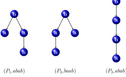
3.2 Some examples of q-grams, with q = 4. Pi identifies the structure of the path, the string the sequence of labels as encountered by visiting the subtree. . . 52

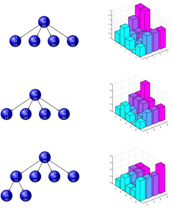
4.1 Example of representation in feature space of three trees according to the Activation Mask Kernel for = 1. On the left part of the image three simple trees and on the right part their activation masks referring to a 5×4 map. The height of each element of the map corresponds to the value of the activation. . . 60

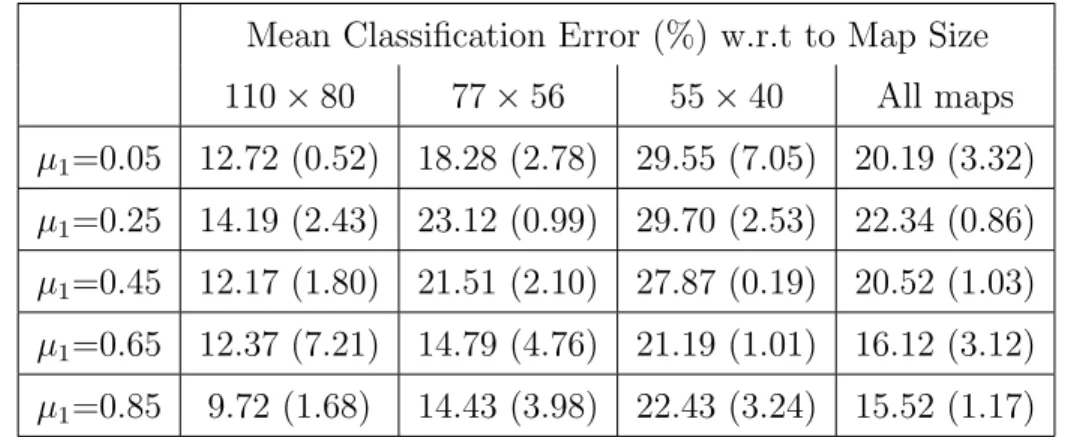
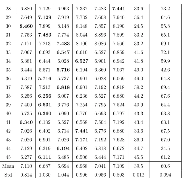
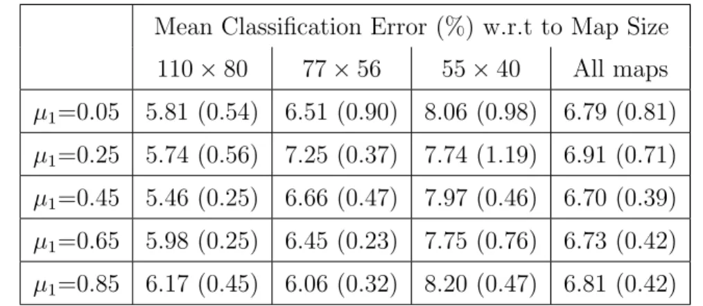
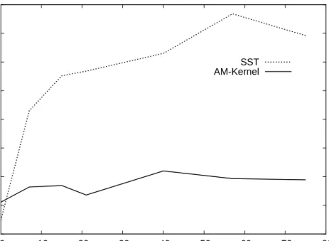
SOM-SD classification error. The error values of the AM-kernel are related to the value selected on validation (which is reported in correspondence of the map error value). . . 71 4.3 Classification error of the SST and AM-kernel on various datasets

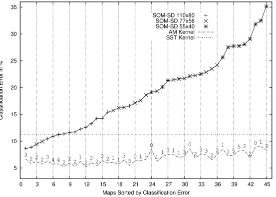
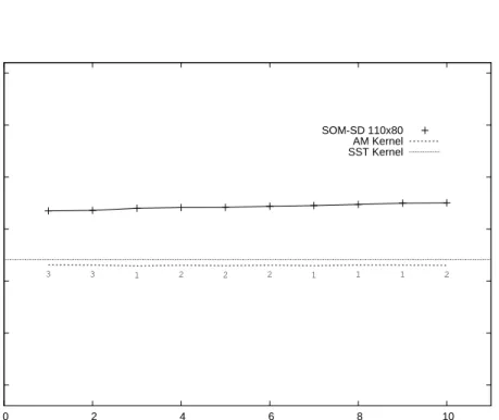
with different levels of sparsity. . . 76 4.4 Comparison between classification error (using 3-fold cross-validation)

of the different techniques on the LOGML test dataset. Maps on the x-axis are sorted by SOM-SD classification error. The error values of the AM-kernel are related to thevalue selected on validation (which is reported in correspondence of the map error value). . . 78 5.1 An example of a route connecting nodes labelled with a and e. The

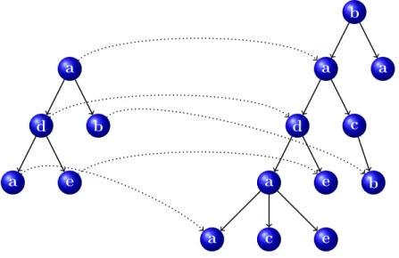
nodes connected by dashed edges are the ones comprising the path between the two nodes. The route is formed by the sequence 2,3 since nodeb is the second child of aand node e is the third child of b. . . 80 5.2 A tree (left) and its set of features according to the route kernel

defined in eq. (5.12). . . 84 6.1 Example of how to represent a forest as a minimal DAG with no loss

of information. Nodes in the minimal DAG are annotated with a label and the frequency in the forest of the subtree rooted at that node.101 6.2 The algorithm to transform a tree-forest into a minimal DAG. . . 102 6.3 The algorithm to insert a weighted ADAG in a larger ADAG. . . 104 6.4 The DAG-Perceptron algorithm. . . 107 6.5 Execution time in seconds for the Standard Perceptron and the Voted

DAG Perceptron using a polynomial kernel with degree 3 (Poly3) over the training set with 992,819 examples. . . 114

for the λ parameter, i.e. λ ∈ {0.3, 0.4, 0.5, 0.6, 0.7, 0.8, 0.9, 1.0}, over the training set with 992,819 examples. For each method, only the fastest and the slower executions are reported. . . 115 6.7 Execution time in seconds for the Standard Perceptron and the Voted

DAG Perceptron using a linear combination of a polynomial kernel with degree 3 (Poly3) with the SST tree kernel (Tk), i.e. (1−γ)∗

P oly3 +γ∗T k, over the training set with 992,819 examples. Different values for λ and γ have been considered, i.e. λ ∈ {0.3, 0.4, 0.5, 0.6, 0.7, 0.8, 0.9, 1.0} and γ ∈ {0.2, 0.3, 0.4, 0.5, 0.6}. For each method, only the fastest and the slower executions are reported. . . 116 6.8 Evolution of the number of tree nodes stored in memory and belonging

to the model developed by the Standard Perceptron and the Voted DAG Perceptron during training on the training set with 992,819 examples. Both methods use the SST tree kernel (Tk) with different values for λ, i.e. λ ∈ {0.3, 0.4, 0.5, 0.6, 0.7, 0.8, 0.9, 1.0}. For each method, only the executions with the largest and the lower number of stored nodes are reported. . . 117 6.9 Evolution of the number of tree nodes stored in memory and belonging

to the model developed by the Standard Perceptron and the Voted DAG Perceptron during training on the training set with 992,819 examples. Both methods use a linear combination of a polynomial kernel with degree 3 (Poly3) with the SST tree kernel (Tk), i.e. (1−

γ)∗P oly3 +γ∗T k. Different values for λandγ have been considered, i.e. λ ∈ {0.3, 0.4, 0.5, 0.6, 0.7, 0.8, 0.9, 1.0} and γ ∈ {0.2, 0.3, 0.4, 0.5, 0.6}. For each method, only the executions with the largest and the lower number of stored nodes are reported. . . 119

the λ parameter, i.e. λ ∈ {0.3, 0.4, 0.5, 0.6, 0.7, 0.8, 0.9, 1.0}, over the union of the INEX 2005 training and test sets. . . 120 6.11 Evolution of the number of tree nodes stored in memory and

be-longing to the model developed by the Standard Perceptron and the Voted DAG Perceptron during training on the union of the INEX 2005 training and test sets. Both methods use the SST tree kernel (Tk) with different values for λ, i.e. λ ∈ {0.3,0.4,0.5,0.6,0.7}. For the Standard Perceptron only the execution with lower number of nodes is reported. For the Voted Dag Perceptron only the execution with the largest number of nodes is reported.. . . 121 A.1 Parse tree of the sentence ”Mary brought a cat to school” along with

the PAF trees for Arg0, Arg1 and ArgM. . . 135

Introduction

Since the advent of modern computers the amount of available information has been increasing more than our capacity of analysing it. The development of automatic tools for data analysis is still an active area of research. Machine learning comprises a series of techniques for automatic extraction of meaningful information from large collections of noisy data.

Traditional methods in machine learning deal with vectorial information even if, in many real world applications, data are naturally represented in structured form (graphs for instance): XML data, molecular structures in chemical informatics, parse trees in natural language processing and protein sequences in bioinformatics.

In order to apply machine learning techniques designed for vectorial data to structured data, a pre-processing phase is required in order to encode structured information into vectorial form. A pre-processing is always task specific and needs to be suitably designed for any new task. The pre-processing can result in the loss of relevant or necessary information for the given task.

Recent developments in machine learning have produced methods capable of processing graph structured information directly. Among these, kernel methods are becoming more and more popular. Being on one hand theoretically well founded in statistical learning theory, they have on the other hand shown good empirical

results in many applications. Kernel methods introduce a novel way of handling structured data since they do not require an explicit representation of each input, they instead require the definition of a kernel, i.e. a similarity function between all pairs of objects of a domain. The definition of kernel functions for structures is a challenging task because of the need to balance the trade-off between accuracy (how well its values represent the true similarity between objects) and its computational complexity.

Kernel methods have proven to be successfully for many real world problems. However, the kernels currently defined in literature have some drawbacks. Investi-gating ways of overcoming current kernel drawbacks and looking for more effective kernels is the main motivation for this thesis.

1.1

What is Machine Learning

One of the main motivations for the development of machine learning techniques is to automatically extract meaningful information from large collections of data: recog-nizing human speech, detect fraudulent credit card transactions, perform automatic medical diagnosis. For a more detailed example consider the case of recognizing tumours in magnetic resonance images (MRI). An MRI exam produces many series of images (up to 6) each one containing many images (more than 30). All of them have to be carefully analysed in order to discover the presence of a tumour. This is a long process and therefore the daily number of examined patients is limited. This problem features two of the issues typically faced by machine learning: data may be noisy and no algorithmic solution is known. In the MRI example a radiologist, in most cases, is able to recognize a tumour but he is not able to formalize the problem and define an exact and generally applicable procedure for solving it. The only way to communicate its knowledge to a student, for example, is to give him a series of images along with their classification (whether they contain a tumour or not) and guide him in its inference process giving feedbacks on his hypotheses. The student improves his capacity of recognizing tumours with experience. The aim of

machine learning is precisely to provide automatic tools to mimic the human ability to improve its behaviour with experience. Another situation in which the use of a machine learning approach to problem solving is appropriate is when the results are subjective. Algorithms able to adapt to user preferences are usually based on machine learning techniques. For example the notion of interesting web site depends on the user, so an intelligent search engine should learn user preferences and return the results based on them.

1.2

Issues in Structured Data Representation

problems the preprocessing phase affects heavily the accuracy of the learner. More-over, to maintain all the structured information, the dimensionality of the resultant vectors may be quite high. This may be a significant drawback considering the fact that many Machine Learning techniques are not able to effectively scale with the dimensionality of the input and therefore their predictive power decreases with increase in the dimensionality of the input. This problem is known as “Curse of Di-mensionality” [6]. To get an idea of the reason for this performance degradation, it is sufficient to consider a space X of dimension d. Suppose thatX is composed by a set of points uniformly distributed. If the number of dimensions of X increases, the number of points necessary to keep the same density must increase exponentially. In other words, the more the dimensions of the input, the more the probability that the data are sparse. A sparse dataset gives in general too few information to build a good classifier. A flat representation for structured data is thus appropriate when knowledge about the domain can be effectively used to select a set of features. When such knowledge is not available, instead of manually trying different encodings, it is desirable to make use of techniques able to directly handle structured data.

1.3

Kernel Methods for Structured Data

The issue of data representation is faced by kernel methods [7,13,48] from a different perspective. Kernel methods avoid to explicitly represent the data into vectorial form since the only information they require is about the similarity of each pair of data items. By definition, kernel methods look for linear relations in the feature space. Input items are compared via dot products of their representation in the feature space. The feature space is a vectorial description of the data according to a predefined set of features. However kernel methods may avoid to directly access the feature space since it can be shown that it is possible to replace the dot product with a kernel function, a symmetric positive semidefinite function which computes the similarity of a pair of items directly in their original space. The advantage of using kernel functions is that huge, even infinite, feature spaces can be used

with a computational complexity not dependent on the size of the feature space but on the complexity of the kernel function. It can be demonstrated that kernel methods, even if they can implicitly make use of very large feature spaces, they do not suffer of the curse of dimensionality since Statistical Learning Theory [65] shows that the generalization capability of a kernel method ultimately depends on the number of misclassified examples in the learning phase. So far we have showed that it can be avoided to access directly the feature space representation of the input examples. The classification of a new example is performed by consider the sign of the application of the kernel function between the example and the classifier (see eq. (2.15)). It can be shown that, if the kernel method satisfies the assumptions of the Representer theorem (see Section 2.3.2), the classifier can be represented as a weighted sum of the training instances (see section 2.2 for details). Thus the classification of an example is performed via a weighted sum of kernel evaluations between the example and a subset of the training instances. Since the representation of the data in feature space is only accessed implicitly when a kernel function between two examples is computed, kernel methods can be applied to any type of input by providing an appropriate kernel function.

Kernel functions have some interesting features:

• the space of kernel functions is closed under operations such as addition and linear combination. It is then very easy to combine data from different sources. For example, when classifying web pages, it would be possible to integrate information from text, images and links by combining the respective kernels.

• If we consider a finite dataset composed by n examples, we can represent the kernel function by a matrix whose size is always n×n, independently from the size of each individual example. This property can be useful when a small dataset of large size examples has to be analyzed.

Kernel methods have proved to be a state of the art technique for many real world problems. They are described in detail in Section 2.3.2. However designing good kernel functions, i.e. fast to compute and expressive (see Section 2.3.4 for

a definition) is an open problem. In the following these two important issues are discussed. Generally speaking, the main goal of this research is to find methodologies to overcome them.

1.4

Thesis Motivations

Kernel function evaluations heavily affect the computational burden of kernel meth-ods. It is therefore important to keep their complexity as low as possible. Unfortu-nately it has been demonstrated that completely expressive kernels for graphs are NP-Hard to compute [54]: for example a kernel k(G1, G2) that takes into account

the similarity of all possible subgraphs of the two graphs G1 and G2 is equivalent

to testing whether G1 and G2 are isomorphic (a problem known to be NP-Hard).

Kernel functions must be a compromise between accuracy of the results and com-putational complexity of the procedure. In the following we try to make clear what we mean with the term expressiveness. One of the most popular kernel for trees is the subtree kernel (see section 3.1.1 for a description). It counts the number of exactly matching subtrees of the inputs. While the restriction to exact match allows the evaluation of the kernel function to be carried out in nlogn time (where n is the number of nodes), it prevents the application on settings in which the labels of the nodes take values from the domain of real numbers, since hardly there will be any matching subtree. When the number of pairs of inputs having non zero simi-larity is very low, the kernel has low expressiveness and is said to be sparse. It is a pathological situation since those kernels are likely to not give enough information to the classifier, which will behave like a nearest neighbour rule [30, 61], i.e. it will not be able to generalize well on unseen data. Even in cases in which the labels of the nodes may only have values from a discrete domain, the subtree kernel may be sparse. For example, we collected some statistics from a dataset of XML data (see section A.1) and noticed that the subtree kernel would have resulted in a 0 kernel value, i.e. inputs totally dissimilar, for the 54.71% of the kernel evaluations. Re-laxing the constraint which allows matchings only between identical subtrees does

not help because the resulting computational complexity of kernel evaluations would make the use of kernel methods infeasible. The development of techniques and ker-nel functions with an acceptable accuracy/complexity trade-off is an open problem and it is one of the main targets for this research.

A second motivation for the development of novel non sparse and expressive kernel functions comes from the analysis of the literature on kernel for trees. Most of them fall under convolution kernel framework, which expresses a kernel on a pair of structures as a combination of kernels on their constituent substructures. However, all those kernels focus on the presence of the substructures and partially discard information about the position of the substructures in the original structure. This observation led us to investigate whether this type of information can be useful.

There are important computational issues not only in the computation of kernel functions, but also in the classification phase. As mentioned earlier, the hypothesish

returned by a kernel method can be expressed as a linear combination of the inputs. To be more precise, h can be expressed as a linear combination of the wrongly classified inputs. In order to use h the whole set of wrongly classified inputs must be kept in memory. While saving in memory a great amount of plain data may be feasible, saving great amounts of structured data, due to the typical increase in size, may severely limit the applicability of the technique. Just as an example, we collected some statistics from an XML dataset [36] finding out that the total number of nodes of the misclassified inputs tended to increase linearly with the size of the training set. It is worth pointing out that the reduction of the computational resources of a kernel method is not only a computational issue, but it also affects the accuracy of the classifier. In fact, in machine learning it is a well known fact that the accuracy of the classifier improves with the size of the training set.

1.5

Outline of the Thesis and Original

Contribu-tions

This section describes the contents of the thesis highlighting its original contribu-tions.

The thesis is divided into two parts. The first part outlines background concepts and gives a survey of the state of the art of kernel for trees.

Chapter 2 introduces the notation and basic concepts used throughout the re-maining chapters. Section2.1gives basic definitions about the structures used in the following chapters. Section 2.2 introduces the Machine Learning framework. Sec-tion 2.3 gives an overview of two approaches for handling tree structured data, the Self Organizing Map for Structured Data and kernel methods. The latter comprises a series of techniques which avoid to explicitly represent the data, since they rely on information about the similarity of objects in a domain. This type of information is given by the kernel functions. Sections 2.3.3 and 2.3.4 describe kernel function properties and discuss the contributions in literature for assessing their quality.

Chapter 3 gives an overview of the kernel functions for tree structured data. Section 3.1 introduces the convolution kernel framework and describes the kernel functions based on it. Section 3.2 gives a overview of other approaches for building kernel functions.

The second part of the thesis is devoted to the presentation of the original con-tribution.

A drawback of the standard tree kernels is that in the case of large structures and many symbols, the feature space implicitly defined by these kernels is very sparse. Chapter 4 proposes a novel family of kernels based on the activation of a Self Organizing Map for Structured Data, a clustering algorithm which maps tree structured information in such a way that similar trees are mapped onto nearby areas to form clusters. Specifically, we make use of this property to design kernel functions able to perform inexact subtree matching thus reducing the sparsity of the original kernel while trying to keep its structural information. Section4.1describes the novel

family of kernels based on Self Organizing Map for Structured Data activations, the Activation Mask Kernel. Section 4.2 discusses the relationships of the new kernel with other kernels defined in literature. Section 4.3 present experiments performed to verify the effectiveness of our approach.

A second contribution was motivated by the observation that convolution tree kernels match substructures without taking into account their “relative positioning” with respect to one another. In chapter 5 a novel family of kernels is defined which explicitly focus on this type of information. Section 5.1 gives a formal definition of the novel kernel and Section5.2describes an instance of the general form. Section5.3 describes the experiments performed in order to establish the effectiveness of the kernel.

While Support Vector Machines has a high generalization capability, a drawback of their use is the time required both in learning and classification phases. As a third contribution, in chapter6we present a methodology for reducing that compu-tational burden for convolution tree kernels by a suitable encoding of the structures which avoid the re-computation of kernels between the same substructures belong-ing to different examples. Section6.1 describes a general methodology applicable to convolution kernels. Section 6.2 describes the application of our idea to the subtree and subset tree kernels and shows experiments proving its effectiveness.

1.6

Origin of the Chapters

The material presented in chapter 4is based on the following articles [2]. Chapter5 is based on unpublished work. Chapter 6is based on the following articles [3, 4].

Basics

Background

This chapter introduces basic definitions and concepts necessary for understanding the works presented in chapters 4,5 and 6. Section 2.1 presents the notation and definitions related to trees. Sections2.2introduces the machine learning framework. Section 2.3 discusses those techniques for learning on structured data that are used in the following chapters. Since the focus of this work is on kernel methods, sec-tions2.3.3introduce basic properties of one of the fundamental components of kernel methods, kernel functions. The chapter ends with section 2.3.4 by discussing ways to evaluate kernel functions.

2.1

Definitions and Notation

This section recalls basic definitions and notation that will be used in the following chapters. We start with some definitions on data structures.

A graph is a pair of sets G= (VG, EG), where VG={v1, vn} is an ordered set of nodes and EG ={eij = (vi, vj), . . . , ekl = (vk, vl)} a set of pairs of nodes, the edges. The subscript G will be omitted whenever it is clear from the context which graph we are referring to. An undirected graph is a graph for whicheij ∈E ⇔eji ∈E. A labelled graph is a graph for which a label is attached to each node. Labels will be represented by means of a function l(v) or, when referring to a specific node vi, by

a

c d

a b

Figure 2.1: An example of a labelled directed graph.

there exists an edge connecting any adjacent nodes, i.e. (pi, pi+1) ∈ E,1 ≤ i ≤ l,

where pi is the i-th node in the path and l is the length of the path (the number of nodes comprising p). Two nodes are connected if there exists a path connecting them. A graph is connected if every pair of distinct vertices in the graph is connected. A graph is said to have a cycle if there exists a path connecting a node with itself, i.e. ∃p=p1, . . . , pl. p1 =pl.

Figure2.1 gives an example of a labelled directed graph. Note that the graph is not connected since there is no path connecting nodes labelled with b and c.

A tree is a directed and connected graph without cycles for which every node has at most one incoming edge. A rooted tree is a tree for which there exists a node with no incoming edges (the root). In order to simplify the notation, we will use

v ∈G has a shortcut for v ∈VG. A leaf is a node with no outgoing edges. If there is a link eij, node vi is the parent of vj and node vj is a child of vi. If vj, vk are children of vi, then vj and vk are siblings. A node vj is a descendant of vi if there exists a path from vi tovj (in this case vi is an ascendant ofvj). An ordered tree is one in which the children of each node are ordered according to some relation.

A positional tree is a tree for which each child node has associated an index representing its position with respect to its siblings. Note that the set of positional trees include the set of ordered trees. Figure 2.2 highlights the differences of an ordered tree with respect to a positional tree: edge labels represent the position of a node. In the following node positions for ordered trees will be omitted. The out-degree of a node is the highest positional index associated to a child of the

a b c e g 2 3 3 1

Figure 2.2: A positional Tree. The number over an arc represents the position of the node with respect to its parent.

a b c e g

⇒

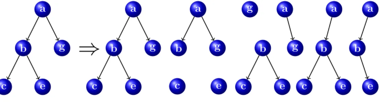
Figure 2.3: A tree (left) and some of its subtrees (right).

node. The maximum out-degree of a tree is the highest index of all the nodes of the tree. The out-degree of a node for an ordered tree corresponds to the number of its children. The depth of a node vi with respect to one of its ascendants vj is defined as the number of nodes comprising the path from vj tovi. When not specified, the node with respect to the depth is computed, is the root.

A tree can be decomposed in many types of substructures.

Subtree A subtree t is a subset of nodes in the tree T, with corresponding edges, which forms a tree. A subtree rooted at node vi will be indicated with ti, while a subtree rooted at a generic node v will be indicated by t(v). When t is used in a context where a node is expected, t refers to the root node of the subtree t. The set of subtrees of a tree will be indicated by NT. When clear from the context NT may refer to specific type of subtrees. Figure 2.3gives an example of a tree together with its subtrees. Various types of subtrees can be defined for a tree T.

a b c e g

⇒

Figure 2.4: A tree (left) and all of its proper subtrees (right).

a b c e g

⇒

Figure 2.5: A tree (left) and all of its subset trees (right).

Proper Subtree A proper subtree ti comprises node vi along with all of its de-scendants (see figure2.4 for an example of a tree along with all its proper subtrees).

Subset Tree A subset tree is a subtree for which the following constraint is sat-isfied: either all of the children of a node belong to the subset tree or none of them. The reason for adding such a constraint can be understood by considering the fact that subset trees were defined for measuring the similarity of parse trees in natural language applications. In that context a node along with all of its children represent a grammar production. Figure 2.5 gives an example of a tree along with some of its subset trees.

2.2

Machine Learning

The machine learning framework encompasses all algorithms capable of improving their behaviour with experience. According to the definition of Mitchell [44], a computer program is said to learn from experience E with respect to some class of tasks T and performance measure P, if its performance at tasks in T, measured according to P, increases with experience E.

Two different scenarios can be distinguished in machine learning: supervised and unsupervised learning. In the supervised scenario a set of pairs, the training set,

S ={(xi, yi) :i= 1, . . . , n} is provided to the learner. xi ∈ X is the input example (X denotes the domain of thexi, X is the set of allxi appearing inS),yi ∈Y is the label of xi. Each (x, y) is generated according to an unknown distribution P(x, y).

S is assumed to be independent and identically distributed according to P(x, y). The domain of Y determines the type of problem (the following list considers only problems of interest for the present work):

• If yi ∈ {0,1} it is a two-class classification problem. It is the simplest case. Most machine learning classification algorithms belong to this class.

• If yi ∈ {0, . . . , n} it is a multi-class classification problem. The prediction of an instance is selected among n+ 1 classes.

• If yi ∈R it is a regression problem. Regression can be viewed as the problem of fitting a curve representing the target function.

• Ifyi ∈ {0,1}m it is a multi-label classification problem: the classification ofxi is a vector where each dimension represent the classification with respect to the corresponding label.

The task in supervised learning is to estimate a functionh:X →Y, representing the relationship betweenxand yvalues, having at disposal only the set of examples

The besth, represented as h∗, minimizes the expected risk:

R(h) = Z

L(h(x), y)dP(x, y) (2.1) where L is a loss function measuring the classification error of h. L can be, for instance, the total number of misclassified examples (binary loss).

Since the distributionP(x, y) is unknown, it is not possible to directly use equation (2.1) for selecting the best h. A reasonable approach is to minimize the loss function with respect to the available data.

Re(h) = 1 n X (x,y)∈S L(h(x), y) (2.2)

The set of h such that R(h) = 0 is called Version Space [44]. This technique alone, however, does not lead to an optimal h since there can be infinite functions for which ∀(xi, yi) ∈ S : h(xi) = yi. The ability of a function to correctly classify unseen data is referred to as generalization capability. It is clearly of particular interest to express the generalization capability of an algorithm without referring to a specific instance of the problem (a specific set of data). Statistical Learning Theory is devoted to this problem. Among its results there is a characterization of the classes of functions with respect to the Vapnik-Chervonenkis (VC) dimension, a measure of the complexity of the class. The VC dimension of a family of functions

H is defined as the cardinality of the largest subset of points of the domain that can be labelled arbitrarily by choosing a function h ∈ H. Loosely speaking the VC dimension grows with the ability of a set of functions to correctly classify any training set. The following theorem shows that the generalization ability of a family of functions decreases when increasing the VC dimension.

Theorem 2.1 Let v be the VC dimension of the family of functions H. Then

∀ δ > 0, h∈H dependent from a set of parameters Θ, the upper bound

R(h(Θ))≤Re(h(Θ)) + Ω VC(h(Θ)) n , (2.3)

where Re is the empirical risk and n is the size of the training set, holds with

prob-ability at least 1−δ for n > VC(h(Θ)). ΩVC(h_n(Θ)) is a monotonic increasing function and it is called the confidence interval.

Note that the generalization ability of an algorithm increases by having at disposal a larger amount of data. The confidence interval is also related to the VC dimension: if a function with low complexity is able to correctly classify the training set, then it is likely to have a low expected risk. The minimization of both terms of eq. (2.3) is important. When a function is able to correctly classify the training set but has a large error on the rest of the distribution, then the function is told to overfit the data. When a function has a low confidence interval but has not enough expressive power (it is not able to correctly classify the training set), it is told to underfit the data.

Since the minimization of the empirical risk alone does not guarantee to obtain high accuracy on the whole distribution, in order to obtain a useful solution, the learning process needs to incorporate a bias, based on a priori knowledge of the problem, for restricting the set of functions from which the selection of the best his performed. Note that, since the choice of the bias is made before seeing the training set, the resulting class of functions, may not contain h∗. On the other side, given a bias, it is possible to build a training set such that any algorithm will perform arbitrarily bad. A priori knowledge may make take the form of

• a restriction of the family H from which h∗ will be selected,

• a penalization for complex functions (Regularization). An example of a reg-ularizer is a penalization term which influence the selection towards smooth functions.

• The selection of a functional class according to the structural risk minimization principle [10]. Let H1 ⊆ H2 ⊆ . . . ⊆Hk be a sequence of family of functions with VC(Hi)< VC(Hi+1),1 ≤i < k. Among those functions minimizing the

empirical risk for each Hi, the structural risk minimization principle chooses the one minimizing also a bound of the form of eq. (2.3).

In the unsupervised learning scenario there is no label information available. The learner is provided with only a set of instances X={xi :i= 1, . . . , n}. The task

here is to find regularities in the set X. The most classical unsupervised technique is clustering, which has the aim of finding a partition of a dataset such that any object of a partition has higher similarity with objects in the same partition than with objects of different partitions.

Machine learning algorithms can be further classified into batch (or off-line) and on-line algorithms. For batch algorithms the distributionP(x, y) generating the data is fixed, while for on-line algorithms it may vary in time. Batch methods have at disposal the whole training set and the learning and classification phase are distinct: once training has finished, the learner has no possibility to modify its behaviour, i.e. to adapt to new examples. In on-line methods data arrives sequentially and learning takes place together with classification. On-line algorithms must be less computational intensive because the two phases, learning and classification, must be executed together.

2.3

Machine Learning For Structured Data

The aim of this section is to describe some of the learning algorithms, applicable to structured data, that will be used in the following chapters.

2.3.1

Self Organizing Maps

The aim of the Self Organizing Maps (SOM) learning algorithm is to learn a feature map

M:I →A (2.4)

which given a vector in the spatially continuous input space I returns a point in the spatially discrete output display space A. This is obtained in the SOM by associating each point in A to a different neuron. Moreover, the output space A

is typically obtained by arranging this set of neurons as the computation nodes of a one- or two-dimensional lattice. Given an input vector xv, the SOM returns the coordinates within A of the neuron with the closest weight vector. Thus, the

set of neurons induce a partition of the input space I. In typical applications

I ≡IRm, wherem 2, andAis given by a two dimensional lattice of neurons. In this setting, high dimensional input vectors are projected into the two dimensional coordinates of the lattice, with the aim of preserving, as much as possible, the topological relationships among the input vectors, i.e., input vectors which are close to each other should be projected to neurons which are close to each other on the lattice. The SOM is thus performing data reduction via a vector quantization approach.

In a more generic case, when the input space is a structured domain with labels in U, we redefine equation (2.4) to be:

M#_:U#[i,o]_{→A (2.5)}

This can be realized through the use of the following recursive definition:

M#(G) =    nilA if G=ξ Mnode us,M#(G(1)), . . . ,M#(G(o)) otherwise (2.6) where s = source(G), G(1)_{, . . . , G}(o) _{are the (eventually void) subgraphs pointed}

by the outgoing edges leaving from s, nilA is a special coordinate vector into the discrete output space A, and

Mnode :U ×A× · · · ×A

| {z }

o times

→A (2.7)

is a SOM, defined on a generic node, which takes in input the label of the node and the “encoding” of the subgraphs G(1), . . . , G(o) according to the M# _{map. By}

“unfolding” the recursive definition in equation (2.6), it turns out that M#_{(G) can}

be computed by starting to apply Mnode to leaf nodes, and proceeding with the application of Mnode bottom-up from the frontier to the supersource of the graph

G.

Model of Mnode

In the previous section we saw that the computation of M# _{can be recast as the}

struc-ture. Moreover, the recursive scheme for graph Gfollows the skeleton skel(G) of the graph. In this section, we give implementation details on the SOM Mnode.

For each node v in VG, we have a vector uv of dimension m. Moreover, we realize the display output space Athrough a q dimensional lattice of neurons. We assume that each dimension of the q dimensional lattice is quantized into integers,

ni, i= 1,2, . . . , q, i.e., A≡[1. . . n1]×[1. . . n2]× · · · ×[1. . . nq]. The total number of neurons is Qq

i=1ni, and each “point” in the lattice can be represented by a q dimensional coordinate vector c. For example, if q = 2, and if we have n1 neurons

on the horizontal axis andn2 neurons on the vertical axis, then the winning neuron

is represented by the coordinate vector y ≡ (y1, y2) ∈ [1. . . n1]×[1. . . n2] of the

neuron which is most active in this two dimensional lattice. With the above assumptions, we have that

Mnode :IRm×([1. . . n1]× · · · ×[1. . . nq])o →[1. . . n1]× · · · ×[1. . . nq], (2.8) and the m+oq dimensional input vector xv toMnode, representing the information about a generic node v, is defined as

xv =

uv ych1[v] ych2[v] · · · ycho[v]

, (2.9)

wherey_chi[v]is the coordinate vector of the winning neuron for the subgraph pointed by the i-th pointer ofv. In addition, we have to specify hownilA is defined. We can choose, for example, the coordinate (−1, . . . ,−1

| {z }

q

).

Of course, each neuron with coordinates vector c in the q dimensional lattice will have an associated vector weight _wc ∈IRm+oq.

Notice that, given a DAG D, in order to compute M#_{(D), the SOM M}

node must be recursively applied to the nodes of D. One node can be processed only if all the subgraphs pointed by it have already been processed by Mnode. Thus, the computation can be parallelized on the graph, with the condition that the above constraint is not violated. A data flow model of computation fits completely this scenario. When considering a sequential model of computation, a node update

scheduling constituted by any inverted topological order for the nodes of the graph suffices to guarantee the correct computation of M#_.

Finally, it must be observed that, even if the SOM Mnode is formally just tak-ing care of stak-ingle graph nodes, in fact it is also “codtak-ing” information about the structures. This does happen because of the structural information conveyed by the

y_chi[v] used as part of the input vectors. Thus, some neurons of the map will be maximally active only for some leaf nodes, others will be maximally active only for some nodes which are roots of graphs, and so on.

Training algorithm for Mnode

The weights associated with each neuron in the q dimensional lattice Mnode can be trained using the following process:

Step 1 (Competitive step). In this step the neuron which is most similar to the input node xv (defined as in equation (2.9)) is chosen. Specifically, the (winning) neuron, at iteration t, with the closest weight vector is selected as follows:

y_i∗(t) = arg min

ci kΛ(xv(t)−mci(t))k, (2.10)

where Λ is a (m+cq)×(m +cq) diagonal matrix which is used to balance the importance of the label versus the importance of the pointers. In fact, the elements λ1,1,· · · , λm,m are set to µ, the remaining elements are set to 1-µ. Notice that ifcq = 0 andµ= 1, then the standard SOM algorithm is obtained. Step 2 (Cooperative step). The weight vector _my

i∗, as well as the weight

vector of neurons in the topological neighborhood of the winning neuron, are moved closer to the input vector:

mcr(t+ 1) =_mcr(t) +η(t)f(∆i∗_r)(x_v(t)−mcr(t)), (2.11)

where the magnitude of the attraction is governed by the learning rate η and by a neighborhood function f(∆i∗_r). ∆_i∗_r is the topological distance between

cr and ci∗ in the lattice, i.e., ∆_i∗_r = kc_r−c_i∗k, and it controls the amount

to which the weights of the neighboring neurons are updated. Typically, the neighborhood function f(·) takes the form of a Gaussian function:

f(∆i∗_r) = exp − ∆ 2 i∗_r 2σ(t)2 (2.12) where σ is the spread. As the learning proceeds and new input vectors are given to the map, the learning rate gradually decreases to zero according to the specified learning rate function type. Along with the learning rate, the neighborhood radius σ(t) decreases as well1_.

Putting this all together, the training algorithm of the SOM-SD can be described as shown by Algorithm 1, where for the sake of notation we denote Mnode by M. We will use this concise notation also in the following.

In this version of the algorithm, the coordinates for the (sub)graphs are stored in

y_v, once for each processing of graphD, and then used when needed2_{for the training}

ofM. Of course, the stored vector is an approximation of the true coordinate vector for the graph rooted in v. However, since the learning rate η converges to zero this approximation can be negligible.

The SOM can be considered as an instance of a general framework for process-ing of structured data [27]. Various extensions of the SOM has been described in literature. The Contextual Self-Organizing Map (CSOM-SD) model family is able to capture contextual information about the input structure, i.e. information about the ancestor of a node [24, 25]. The Graph SOM-SD model allows the processing of undirected graphs, and non-positional graphs where the order of edges is not relevant [26].

The heuristic nature of the SOM-SD can not formally guarantee to preserve the topology of the items in the input space. In order to overcome this limitation, 1_{Generally, the neighborhood radius in SOMs never decreases to zero. Otherwise, if the} neigh-borhood size becomes zero, the algorithm reduces to vector quantization (VQ).

2_{Notice that the use of an inverted topological order guarantees that the updating of the} coor-dinate vectors xv is done before the use ofxv for training.

Algorithm 1: Stochastic Training Algorithm for SOM-SD

input: Set of training DAGsT ={Di}i=1,...,N,omaximum outdegree of DAGs inT, mapM,N iter

number of training iterations,µstructural parameter,η(0),σ, network size;

begin

initialize the weights forMwith random values from withinU; fort= 1toN iter

shuffle DAGs inT;

forj= 1toN

List(Dj)←an inverted topological order for vert(Dj);

for v←first(List(Dj))tolast(List(Dj))do

yv←arg min[a,b]

µkuv−m(l)_[a,b]k+ (1−µ)ky_ch[v]−m(r)_[a,b]k; foreach m[c,d]∈ Mdo m(l)_[c,d]←m(l)_[c,d]+α(t)f(∆[c,d],y_v) (m(l)_[c,d]−uv); m(r)_[c,d]←m(r)_[c,d]+α(t)f(∆_[c,d],y v) (m (r) [c,d]−ych[v]); returnM; end

Gianniotis and Tino [20] have proposed a model based approach for constructing topographic maps of tree structured data. The model is formulated as a constrained mixture of hidden Markov tree models. The maps are formulated in a principled framework of probability theory and thus are more theoretically grounded than SOM-SD.

2.3.2

Kernel Methods

The class of kernel methods comprises all those algorithms that do not require an explicit representation of the examples but only information about the similarities among them. The information is given by the kernel functions (for a definition see Section 2.3.3). Any kernel method can be decomposed into two modules:

• a problem specific kernel function.

• A general purpose learning algorithm.

Since the solver interfaces with the problem only by means of the kernel function, it can be used with any kernel function, and vice versa. The modularity of the approach allows to study the two aspects of learning, i.e. representation and optimization, independently.

Kernel methods look for linear relations in the feature space. In the following, for simplicity, the task of classification is considered. The problem is generally expressed as a constrained optimization problem where the objective function usually take the form of eq. (2.3). If the kernel function employed is symmetric positive semidefinite the problem is convex and thus has a global minimum. Note that a global minimum of the cost function exists for any choice of the parameters and kernel function. Thus the global minimum does not correspond to the optimal solution for the problem.

Wahba’s representer theorem [67] states that the solution of certain optimiza-tion problems involving an empirical risk term and a quadratic regularizer can be written in terms of an expansion of the training examples. Thus, given a dataset

S ={(xi, yi) :i= 1, . . . , n} and a kernel functionK, the solutionw of the problem can be expressed as:

w= n X

i

αiyiφ(xi). (2.13) Before showing how to classify an example, the score function must be introduced:

S(x) = hw, xi= n X i αiyiφ(xi)φ(x) = n X i αiyiK(xi, x). (2.14) Note that the score function can be expressed as a weighted linear combination of kernel function evaluations between examples in the dataset andx. The classification

c(x) of an example with respect tow and kernelK is the sign of the score function:

c(x) = sign(S(x)) =sign n X i αiyiK(xi, x) ! , (2.15)

The two modules comprising kernel methods, i.e. representation and problem optimization, are discussed in detail in the rest of the chapter. The following two sections describe the kernel methods used in the following: the perceptron and the Support Vector Machines, respectively. Note that the two algorithms are for binary classification problems, but they can be applied to an n-class problem by adopting the one-against-all methodology: firstn binary classifiers, each devoted to recognize a single class, are trained. Then, the prediction for the n-class problem is given by the class whose associated classifier gets the highest confidence (score).

Perceptron

In the original formulation the perceptron [56] was meant to classify data encoded by real vectors with a linear decision function (a hyperplane).

Every element of the dataset is represented by a feature vector. A prototype vec-torwis randomly initialized. Then the classification of each examplexi is compared to the one made by the prototype, computed according to the following formula:

If the perceptron is classifying uncorrectly the example then a new prototype w0 is generated from w:

w0 =w+αyixi

where α is a constant (α > 0), yi ∈ {−1,1} is the class of xi. The algorithm has been demonstrated to converge to the optimal hyperplane provided that the data are linearly separable [51].

Using the kernel trick it is possible to extend the perceptron to generate a non-linear decision function and/or to treat structured data by using kernels (see for example [37]).

The on-line kernel-perceptron algorithm, adapted to tree-kernels, requires to maintain an implicit representation of the vectorwin the feature space. Specifically, this corresponds to keep in memory the set of the already seen examples for which the perceptron prediction was erroneous.

Thus we can consider the set of examplesM ={(xi, yi)∈S :αi ∈ {−1,+1}}as the model of the perceptron and slightly redefine the kernel-perceptron algorithm as in the following. Let M =∅ be an initial empty model, a new examplexi is added to the model M whenever its score

S(xi) = X

(xj,yj)∈M

yjK(xi, xj)

has different sign from its classification yi. Thus the update and the insertion of the new example follow the rule:

if (yiS(xi)≤0) then M ←M ∪ {(xi, yi)}

For many applications (see page 35), the cardinality of M, and consequently the memory required for its storage, grows up linearly with the number of tree presen-tations. Moreover the efficiency in the evaluation of the function S(x) decreases super-linearly. Clearly, this seems not satisfactory for on-line applications.

The perceptron is a simple and relatively fast algorithm. Its main drawback is that it does not provide bounds on the generalization error.

An interesting and effective variant of the simple Perceptron algorithm is the

voted Perceptron proposed in [18]. This algorithm is motivated by a theory related to converting an on-line learning algorithm into a batch one. Basically, it uses a deterministic version of a simple “leave-one-out” method whose randomized version was proposed in [29]. Specifically, the idea of the voted perceptron is to combine the predictions of the hypotheses visited by the Perceptron algorithm while its training takes place. These hypotheses can be combined in different ways, for example each hypothesis can be given a weight equal to the number of times the same hypothesis has ’survived’, i.e. the number of iterations until the next mistake has been made.

Support Vector Machines

Support Vector Machines (SVMs) are based on the Structural Risk Minimization principle for which bounds on the generalization error have been proven [65]. SVM is a binary classifier which projects the examples in a feature space and then looks for an hyperplane separating positive and negative examples. Among the hyperplanes separating the data, it is chosen the one maximizing the margin, i.e. the minimum distance between the hyperplane and the closest example. It is possible to show that the VC dimension of a linear classifier can be upper bounded in terms of the margin [65]. If the training set is linearly separable the separating hyperplane maximizing the margin is unique and corresponds to the solution of the following problem: arg minw,b ||w||2 2 subject to∀(xi, yi)∈S.yi(w·φ(xi)) +b ≥1 (2.16) where w and b define the hyperplane in the feature space. Considering that the margin is inversely proportional to the norm of w, minimizing ||w|| corresponds to finding the less complex function satisfying the constraints in 2.16, i.e. the simplest function correctly classifying each example. The representer theorem [57] states that the solution f of the problem 2.16 can be expressed as:

∀x∈ X.f(x) = X xi∈S

The examples for which the corresponding α is not 0 are called support vectors. When the training set is not linearly separable, a functionf separating the two classes may be very complex. If the non linear separability is due to noise, perfect classification of the training set is not desirable since it may overfit the data and thus reduce the expected risk. In this case a tradeoff between function complexity and minimization of training error (constraints satisfaction) should be pursued. The problem 2.16 then becomes:

arg minw,b,ξ ||w||2 2 +c Pn i=1ξi subject to ∀(xi, yi)∈S. yi(w·φ(xi)) +b≥1−ξi ξi ≥0 i= 1, . . . , n (2.17)

The constraints in 2.17 are relaxed with respect to the correspondent constraints in 2.16. The parameter c determines the balance between minimization of training error and minimization of expected risk. The parameter is problem dependent and its best value has to be found empirically.

2.3.3

Kernel Functions

A way for assessing the similarity of objects of a domain is to describe them by a set of features and then count the number of common features. For reasons that will be clear in the following, the space of the features is assumed to be a metric space. A metric space X is a vector space in which a distance d:X×X →_R+ _{is defined}

such that ∀ x, x0, x00∈X the following properties hold:

• d(x, x0)≥0

• d(x, x0) = 0⇔x=x0

• d(x, x0) = d(x0, x)

• d(x, x0)≤d(x, x00) +d(x00, x0).

The representation in feature space is obtained by the application of an appropriate function φ, x → φ(x) = {φi(x)|i ≥ 1}. The elements φi(x) are called the features

of x (according to the mapping φ). Note that if φ is a non linear function, the relative positioning of the objects in the feature space can change with respect to the original space. In this sense the use of appropriate kernel functions may (and it is supposed to) simplify the problem.

The similarity between two objects x, x0 can be computed by the dot product of their representation in feature space i.e. hx, x0i = Pm

i = φi(x)φi(x

0_{), where}

m =|φ(x)|. A kernel is a function measuring the similarity of any pair of objects of a domain, K :X × X →_Rwhich corresponds to a closed form for the dot product of the projection of the examples in feature space.

The Gram matrixGK related to a kernelK with respect to a set S of examples is defined as

GK_i,j =K(xi, xj). (2.18) A kernel function is valid if and only if it is symmetric semidefinite positive, i.e. if any of its Gram matrices are symmetric positive semidefinite. A matrix is symmetric if∀i, jK(xi, xj) =K(xj, xi) and it is positive semidefinite if∀c1, . . . , cn∈ R.

X

i,j

ciK(xi, xj)cj = cTGKc ≥ 0, where cT is the tranpose of c. Equivalently a matrix is positive semidefinite if all of its eigenvectors are nonnegative. A kernel function can be expressed as a dot product in a feature spaceφsuch thatK(xi, xj) = P

iφn(xi)φn(xj).

In the following, when it is clear from the context we will use the term kernel in place of valid kernel.

Given two examplesxi and xj, the relationship between the distanced(xi, xj) in feature space and the kernel K(xi, xj) is

d(xi, xj) = q

K(xi, xi) +K(xj, xj)−2K(xi, xj).

When two examples are mostly dissimilar, the application of a kernel K to them returns 0. When the kernel is normalized (see eq. (2.19)) the maximum value of K

is 1.

The class of kernel functions is closed under the operations described in propo-sition 2.1.

Proposition 2.1 Let K1, K2 :X × X →R be two kernel functions,

X ={x1, . . . , xn} a set of examples from the domain χ. Then

1. K(x, x0) = K1(x, x0) +K2(x, x0) is a valid kernel [59] (additive property).

2. K(x, x0) = K1(x, x0)K2(x, x0) is a valid kernel (multiplicative property). Note

that the property holds when K2 is a positive constant, i.e. multiplying the

kernel by a positive constant gives a valid kernel.

3. K(x, x0) = f(x)f(x0), where f is any function defined on the domain χ. 4. K(x, x0) = K4(φ(x), φ(x0)). An application of this property is shown together

with the definition of the polynomial kernel (eq. (2.21)).

5. K(x, x0) = K1⊕K3((x, u)(x0, u0)) =K1(x, x0)+K3(u, u0), where K3 :U×U →

R is a valid kernel defined on the domain U, is a valid kernel (direct sum

property).

6. K(x, x0) = K1⊗K3((x, u)(x0, u0)) =K1(x, x0)K3(u, u0), whereK3 :U×U →R

is a valid kernel defined on U, is a valid kernel (tensor product property).

The proofs of the properties (or references to them) can be found in [28, 59]. These properties show that novel kernels can be defined by combining existing kernels. It is possible to combine kernels taking into account different aspects of the data, for example a kernel for web pages can be constructed by the combination of a kernel defined on the set of words in the page and a kernel defined on the incoming and outgoing links.

When only the orientation of theφ matters, the representation in feature space and thus the kernel values can be normalized by the following operation:

K0(x, x0) = K(x, x

0₎

p

K(x, x)K(x0_{, x}0₎ (2.19)

Normalization can be useful when the probability of generating a feature depends on the size of the original data. For example a representation that counts the number

of times each label appears in a tree is influenced by the size of the tree: larger trees have higher chances to have many common features with any small tree.

In the following we give some examples of popular kernels for vectorial data. Probably the simplest approach for dealing with structured data is to first transform it to vectorial form and then apply kernel functions defined for vectorial data. This section briefly reviews kernels for vectorial data. In the following we may generically refer to kernels defined in this section as standard kernels.

In the following x, y represent vectors belonging to a space _Rm_{. The simplest} kernel known in literature is the linear kernel:

K(x, y) =hx, yi. (2.20)

Note that feature space of the linear kernel coincides with the input space. Another widely used kernel for structured data is the polynomial kernel:

K(x, y) = (hx, yi+e)d, e∈_R, d∈_N. (2.21) The feature space associated with the polynomial kernel is composed by products of elements of the original vectors. dis the maximal order of the resulting monomials. When e = 0, the feature space is composed by all possible products of groups of d

features. Thus the feature space has dimension:

|φ(x)|= n+d−1 d = (n+d−1)! (n−1)!d! .

For example given a vector x = (x1, x2, x3) its representation in feature space for

e = 0 and d = 2 is φ(x) = (x2 1, x22, x23, √ 2x1x2, √ 2x1x3, √ 2x2x3). Note that |x|+ 2

operations are required for evaluating eq. (2.21), while an explicit evaluation by means of the feature vectors φ(x) would have required n+_dd−1operations. The dot product of eq. (2.21) can be replaced by any kernel function (see page 31). The resulting operation allows to create new features as a combination of the original ones.

The last function we describe is the gaussian kernel,

K(x, y) =exp −||x−y|| 2 2σ2 , σ∈_R. (2.22)

The gaussian kernel has the particularity to have a feature space of infinite size. Note that in this case the use of a kernel function not only saves computational time, but it is the only way for computing the corresponding dot product in feature space. The kernel value is maximum when x =y, K(x, x) = 1 and it is monotonic decreasing when the distance between x and y increases. The parameter σ affects the resulting feature space as follows:

• for very high values of σ, all examples become almost parallel and thus all examples are almost identical.

• Very low values of σ produce feature vectors all orthogonal to each other. In [30] the effects of feature spaces such as those obtained for the gaussian kernel for extreme values of σ, on a kernel method called ν-Support Vector Machine [58], are described in detail.

Kernel functions described in this section are suitable for dealing with vectorial data. The present work is focused on tree structured data. The kernels described in literature for this type of data are discussed in section 3.

2.3.4

Evaluating Kernel Functions

It is clear from previous discussions (cfr section 2.3.2) that designing “good” kernel functions is a major concern for obtaining a successful application. But what is a good kernel function? This section summarizes the contributions in literature for helping answering this question. All the following discussion refers to the classifica-tion problem.

Being valid is a necessary requirement for a kernel function. However not all valid kernels all equally good for a task. For example a kernel such that ∀xi, xj ∈

X, i6=j.K(xi, xj) = 0 is a valid kernel but will have a poor generalization capability because no information is available for points in feature space except for those in the training set. We formalize the concept by introducing the sparsity index

Sparsity(K, S) = |{(i, j)∈S|K(i, j) = 0}|

The sparsity index computes the proportion of example pairs in the instance set S

whose kernel value is 0.

On the contrary, given a set of examples xi along with their classification yi (assume for simplicity to be solving a two-class classification problem), it is easy to design a valid optimal kernel: K(xi, xj) =yiyj.

Cristianini et al. [14] have defined a measure for assessing the appropriateness of a kernel function in a supervised setting called kernel alignment. Let S =

{x1, x2, . . . , xn} be the set of instances compounding a training set and K1, K2

two kernel functions defined on S. The empirical alignment between K1 and K2 is

defined as the Frobenius inner product between the corresponding normalized Gram matrices(see eq. (2.18)): A(K1, K2, S) = GK1_{, G}K2 F p hGK1_{, G}K1i FhGK2, GK2iF , (2.24) where GK1_{, G}K2 F = n X i,j=1 GK1 i,jG K2 i,j.

Values ofArange from−1 to 1. The higher the value ofA(K1, K2, S), the higher

the similarity between K1 and K2 with respect to S.

The value A can be used to measure how appropriate a kernel K is for a given two-class classification task by aligning K with a matrix Y defined as: Yi,j =yiyj, where yi = {−1,+1} is the class associated to an instance xi. In the case of a multiclass classification task Y can be defined as Yi,j = 1 if yi =yj and Yi,j = 0 if

yi 6= yj. Note that the codomain of A for the multiclass case ranges from 0 to 1. In [33] the notion of alignment is extended to the case of classification of unbalanced datasets and the problem of regression.

G¨artner [19] defined three properties that should be fulfilled by a good kernel: completeness, correctness, appropriateness. Letc:X →Ω be a function that assigns to every example of a domain its class. Functionscare grouped into a concept class

C.

A kernel that is able to incorporate all necessary knowledge for solving a problem is said to be complete. A kernel is complete if no pair of different examples have the

same representation (in terms of the kernel): K(xi,·) = K(xj,·) ⇒ xi = xj. Any kernel for structured data that discards information about the structure is hardly complete. When information about class membership is available, the constraint

xi =xj can be relaxed thus turning the definition into: ∀c∈C.K(xi,·) = K(xj,·)⇒

c(xi) =c(xj).

A kernel is said to be correct with respect to a concept classC and an hypothesis space, if for every concept can be found an hypothesis that correctly classifies all examples. In the case of the Support Vector Machines, the hypothesis space is composed of all linear functions in feature space. Thus the definition of correctness become: ∀c ∈ C,∃αi ∈ R, xi ∈ X, θ ∈ R such that ∀x ∈ X.

P

iαiK(xi, x) ≥ θ ⇔

c(x).

Appropriateness refers to the extent to which examples that are close to each other in class membership are also close to each other in feature space. A kernel is appropriate for learning concepts in a given concept class by a learning algorithm if polynomial bounds on its generalization error can be derived for some algorithms using this kernel. A complete and correct kernel separated the concept well, i.e. it is able to achieve high accuracy on the given data. An appropriate kernel is able to generalize well to unseen data.

All previous discussions take into account the quality of a kernel. When back-ground knowledge cannot drive the choice of substructures, an effective kernel may be obtained by arbitrarily enlarging the feature space. However using a exponen-tial number of features without having a polynomial kernel function for implicitly computing the dot products between examples may lead to intractable algorithms. The reasoning is valid not only for extreme cases. Even quadratic kernel complexity, in some practical situations, can lead to unacceptable running time. The reason is that, for most complex (and usually more accurate) kernel methods, kernel function evaluations heavily affect the total running time of the algorithm. In order to give an illustrative example of this claim, we computed some statistics on an execution of the Support Vector Machines algorithm (see section 2.3.2) by using the svm-light software [32, 45, 47] on the dataset from INEX 2005 Competition (a description of

the dataset can be found in section A.1). The problem