Algorithms for Projection-Pursuit
Robust Principal Component Analysis
C. Croux
∗,
P. Filzmoser
†and
M.R. Oliveira
‡∗Christophe Croux, University Centre of Statistics and Faculty of Economics and Applied Economics,
K.U. Leuven, Naamsestraat 69, B-3000 Leuven, Belgium; [email protected].
†Peter Filzmoser, Dept. of Statistics & Probability Theory, Vienna University of Technology, Wiedner
Hauptstraße 8-10, A-1040 Vienna, Austria; [email protected].
‡M. Rosario Oliveira, Department of Mathematics and Center for Mathematics & its Applications,
Algorithms for Projection-Pursuit Robust Principal
Component Analysis
Abstract
The results of a standard Principal Component Analysis (PCA) can be affected by the presence of outliers. Hence robust alternatives to PCA are needed. One of the most appealing robust methods for principal component analysis uses the Projection-Pursuit principle. Here, one projects the data on a lower-dimensional space such that a robust measure of variance of the projected data will be maxi-mized. The Projection-Pursuit based method for principal component analysis has recently been introduced in the field of chemometrics, where the number of variables is typically large. In this paper, it is shown that the currently available algorithm for robust Projection-Pursuit PCA performs poor in presence of many variables. A new algorithm is proposed that is more suitable for the analysis of chemical data. Its performance is studied by means of simulation experiments and illustrated on some real data sets.
Keywords: Multivariate Statistics, Optimization, Numerical Precision, Outliers, Robustness, Scale Estimators.
1
Introduction
Projection-Pursuit (PP) methods aim at finding structures in multivariate data by pro-jecting them on a lower-dimensional subspace [1]. PP methods are well suited for the analysis of data sets with a large number of variables, often encountered in chemometrics, since they involve a dimension reduction step. The lower-dimensional subspace, often of
dimension one, is selected by maximizing a certainProjection Index. Principal Component
Analysis (PCA) is an example of the PP approach. If we have n observations x1, . . . ,xn,
all of them column vectors of dimensionp, then the first principal component is obtained
by finding the unit vector a which maximizes the variance of the data projected on it:
a1 = argmax
kak=1
S2(atx
1, . . . ,atxn), (1)
where S2 stands for the variance. By projecting the data on the direction a
1, we obtain
univariate data at
1x1, . . . ,at1xn, in accordance with the Projection-Pursuit idea. Taking
the variance as a projection index leads, as well known, to standard PCA. However, the outcome of standard PCA is very sensitive to atypical observations, e.g. gross errors or sources of new variation. Hence there is a need for robust principal components, yielding
reliable results in presence of outliers, and describing well the structure of the majority of the data.
One of the most appealing procedures for robust PCA was proposed by Li and Chen [2], and is based on the PP principle. The idea is very simple: instead of taking the
variance as a projection index in (1), a robust measure of variance is taken. It was shown
in [2] and [3] that these estimators are consistent and asymptotically normal, and recently [4] proved its robustness by computing influence functions and breakdown points. This approach to robust PCA was introduced in the chemometrics literature by [5] and [6], and was shown to be appropriate for use in chemometrical data analysis. Recently, it was included in TOMCAT, a MATLAB toolbox for multivariate calibration techniques [7]. A recent review on robust statistics in data analysis is given in [8].
The topic of this paper is the actual computation of the principal components, i.e.
solving the maximization problem in (1). When the projection index is the usual standard
deviation, then it is known that a1 is the eigenvector of the sample covariance matrix of
the data corresponding to the largest eigenvalue (see e.g. [9]). But for other choices of
S, solving (1) is not easy, and one needs to rely on approximative algorithms. A first
algorithm was introduced by Li and Chen [2] which, however, was complicated, time consuming, and not made publicly available. In [10] simulated annealing was used, again yielding a slow algorithm that is not publicly available. On the other hand, [11] introduced an algorithm which is very simple, fast to compute and easy to implement. We call it the CR algorithm and consider it as the basis algorithm. Equivalent, but numerically more stable versions were implemented by [5] and [4], see also the discussion in [12]. In this paper we will work with the CR algorithm as described in [4], but [5] and [12] share the same properties, and give exactly the same outcomes, upon rounding error. It was never noticed, however, that the CR algorithm may implode in presence of many variables, making it less suitable for the typical high-dimensional chemometrical applications. This implosion results in a severe downward bias of the scale estimators. This paper will propose a new algorithm not suffering from this problem, being much more precise, while still being computationally efficient. We call this new algorithm the GRID algorithm.
Other proposals, besides the PP approach, have been made for robust PCA, as in [13], [14], or [15]. We would like to emphasize that this paper is not on a comparison between
different types of estimators for robust PCA, since such a comparison was already made
in the aforementioned papers. This paper is on a comparison between differentalgorithms
for computing the PP based estimator defined by (1). We recall that the PP approach
has a clear definition, is intuitively appealing, and has good statistical and robustness properties. It can be applied if the data set has more variables than observations, a case
of special interest in chemometrics. A particular feature is that the PP based approach for PCA allows sequential estimation of the principal components. If we have already
computed the (k −1)th principal component, then the direction of the kth component,
with 1< k≤p, is defined as the unit vector maximizing the indexS2of the data projected
on it, under the condition of being orthogonal to all previously obtained components:
ak= argmax
kak=1,a⊥a1,...,a⊥ak−1
S2(atx
1, . . . ,atxn). (2)
Hence, one is not obliged to compute allp different principal components, but could stop
after, for example, k= 2 steps, implying a significant reduction in computation time if p
is large.
In Section 2 of this paper we briefly review the CR algorithm and in Section 3 we prove that it suffers from implosion in presence of many variables. Section 4 outlines the
new GRID algorithm for finding the optimum values in (1) or (2). Section 5 compares the
different algorithms through some numerical experiments. It turns out that the GRID algorithm finds, throughout practically all experiments, the highest values for the
max-imum in (1), at a reasonable computational price. We also compare the performance of
the algorithms on some real data examples.
2
Description of the Croux-Ruiz (CR) Algorithm
The input of all algorithms we will discuss is a data matrix X withn rows (observations)
and pcolumns (variables), having the observationsxi = (xi1, . . . , xip)t in its rows. Let us
first state that if there are more variables than observations, hence p > n, the first step
of any algorithm we discuss is to perform a singular value decomposition, and continue
working with the scores on all components in ann dimensional space. This is a standard
preprocessing step, yielding no loss of information since we keep the full rank of the data
matrix, e.g. [6]. Hence, we may assume without loss of generality that p ≤ n when
describing the algorithms.
An algorithm will give us a sequence of approximations for the unit vectors defined
by (1) and (2), but also a sequence of maximal values for the (robust) variances, which
we denote by
λk =S2(atkx1, . . . ,atkxn), (3)
for 1 ≤ k ≤ p. If we take for S2 the sample variance, then the values of λ
k are the
eigenvalues of the sample covariance matrix, sorted from the largest to the smallest. For
a robust PCA, we will consider robust versions ofS2, but we will continue to call theλ
as defined by (3), “eigenvalues”. Similar as in [4], [5], and [6], we focus on two particular choices: the Median Absolute Deviation (MAD),
MAD(z1, . . . , zn) = 1.48 med
j |zj −medi zi|, (4)
and the first quartile of the pairwise differences between all data points
Q(z1, . . . , zn) = 2.22{|zi−zj|; 1≤i < j ≤n}((n
2)/4), (5)
where {z1, . . . , zn} is any given univariate data set (see [16]). Taking the squared MAD
or Q, yields then a robust variance estimator. The reason why the MAD or the Q
estimators are taken is that they attain, as a scale estimator, the maximal breakdown point of 50%. The breakdown point is the most popular measure of robustness of an estimator. It measures the smallest fraction of outliers in the data that is needed to drive the scale estimators to their extreme values, i.e. zero for breakdown to zero, and infinity for explosion breakdown.
Before starting the algorithm, we center the data by subtracting the centers of the vari-ables from the columns of the data matrix. Since the arithmetic mean is not robust,
the centering is done with theL1-median [17] or the coordinate-wise median, denoted by
ˆ
µ(X). Note that a fast and stable algorithm for computing an L1 algorithm is described
in [18]. We obtain then the centered data x1
i =xi−µˆ(X). Suppose that in step k−1,
the algorithm returned the vector ˆak−1, an approximation for the solution to (2). Then
we project the observations on the space spanned by the firstk−1 optimal directions, by
computing xk i =xki−1− ¡ ˆ atk−1xk−1 i ¢ ˆ ak−1, (6)
for 1≤i≤n andk > 1. When searching for thekth optimal direction, the CR algorithm
is not optimizing over the whole space of all possible unit vectors, but only considers n
trial directions in the set
An,k = ½ xk 1 kxk 1k , . . . , x k n kxk nk ¾ . (7)
(Elements in An,k corresponding to a zero denominator are set equal to zero.) The kth
eigenvalue is then approximated by ˆ
λk= maxa
∈An,kS 2(atxk
1, . . . ,atxkn), (8)
and ˆak is the argument where the maximum in the above equation is attained.
For more details on the algorithm we refer to [4]. This basic and simple algorithm works well for a large sample size relative to the number of variables, because the set
of trial directions that the algorithm considers are pointing in the directions where the data are. This algorithm has been successfully used in different applications (e.g. [19], [20], [21], [6], [22]). However, due to its construction, the CR algorithm may implode in situations with a low sample size relative to the number of variables.
3
Implosion of the CR algorithm
In this section we will show that the CR algorithm suffers from severe downward bias. In
fact, from a certain orderk on, all estimated eigenvalues will be zero, independently of the
data. We will formally prove that if k > n/2, then ˆλk = 0 when using the CR algorithm.
This is not only happening when taking forS the MAD or the Q, but for any robust scale
measure with a high breakdown point. This implosion of the eigenvalues occurs for all
data sets, whether there are outliers present or not, whatever the latent structure in the data is. This is an undesirable artefact of the CR algorithm.
For stating the next proposition, we need a condition on the scale estimator S. A
scale estimatorS has the m-exact fit propertyif S(Z) = 0 for any sampleZ containing at
least m zeros.
Proposition 1 If a scale estimatorS has them-exact fit property, then the CR algorithm yields at any given data set
ˆ
λk = 0 for k =m+ 1, . . . , p.
Proof: DenoteXk ={xk
1, . . . ,xkn}, where the notation of Section 2 is used. We will first
show by induction that
(A) Xk contains at least (k−1) zero vectors 0.
For k = 1, the property obviously holds, and suppose now that (A) holds for k−2. It
follows from equation (6), that if xk−1
i = 0, then also xki = 0, yielding already k −2
zeros. Denote now i0 the index corresponding to the maximum over the set A
n,k−1 in (8),
so ˆak−1 = xki0−1/kxki0−1k. But then it follows directly from (6) that xki0 = 0. This yields
the (k−1)th zero, and confirms (A).
From (8) it follows that, in the kth step of the CR algorithm, S is computed on a
sample containing k−1 zeros, and this for every value of a. Hence, we conclude that if
S has them-exact fit property with m≥k−1, then ˆλk = 0. ¤
From the definitions (4) and (5) of the MAD and the Q scale estimators, it is easy
observations are equal to each other. Hence Proposition 1 applies for MAD and Q with
m = n/2. In fact, any other robust scale estimator will suffer from the artefact of the
CR algorithm. Indeed, a scale estimator is robust, among others, if its value cannot become arbitrary large in presence of a certain number of outliers. This is formalized by
its explosion breakdown point (cfr. [23], [16]), which at a given sample Z = {z1, . . . , zn}
is defined as
ε∗(S, Z) = min{m
n; supZ0 S(Z
0) =∞} (9)
where Z0 is a contaminated sample obtained by replacing any m observations of Z by
arbitrary values. This next proposition makes a link between the explosion breakdown
point of a scale estimator and the exact fit property of a scale estimator. The relation
between the exact fit property and the breakdown point of an estimator was established for regression estimators by [24], but not yet for scale estimators. Recall that a scale
estimator is said to be scale equivariant if S(az1, . . . , azn) = |a|S(z1, . . . , zn), for any
scalara and any samplez1, . . . , zn. Scale equivariance is a basic property that all sensible
scale estimators share.
Proposition 2 If a scale equivariant scale estimator S has breakdown point ε∗(S, Z) >
(m−n)/n, then it has the m-exact fit property.
Proof: Suppose thatS does not have them-exact fit property. Then there exists a sample
of the formZ ={0, . . . ,0, z1, . . . , zn−m} such thatS(Z)>0. Now replace the last n−m
observations, simply by multiplying them by a factorλ. Denote the contaminated sample
Z0
λ. Then, due to the scale equivariance, S(Zλ0) = λS(Z). Since S(Z)>0, we can let the
scale at the contaminatedZ0
λ tend to infinity, simply by lettingλ tend to infinity, causing
explosion breakdown. Due to the given lower bound on the explosion breakdown point of
S, this cannot occur. Hence there is a contradiction, and them-exact fit property should
hold. ¤
Any robust scale estimatorShaving the maximal value for the breakdown point, being
50% (e.g. [25]), will according to the above proposition have the m-exact fit property,
with m≈n/2. Hence the CR algorithm will also implode for other choices of S having a
high breakdown point, and not only for the MAD or Q estimator.
We also stress that the RAPCA algorithm proposed by [5] suffers from exactly the same implosion problem. The reason is that the CR and the RAPCA algorithm are mathematically equivalent, and they differ only upon rounding error. The data deflation step is done differently in [5], but it is immediate to see that property (A) in the proof of proposition 1 also holds for the RAPCA algorithm. Note that the CR algorithm as
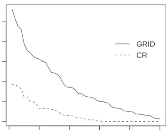
0 10 20 30 40 50 0 50 100 150 200 250 Component number Eigenvalue GRID CR
Figure 1: Scree plot of an artifical data set. For the CR algorithm the eigenvalues are strongly biased, and implode afterk = 30. For the new GRID algorithm no implosion is observed.
described in Section 2 will be faster to compute than the RAPCA algorithm, as was noticed by [6].
In Figure 1 we illustrate the implosion behavior of the CR algorithm. We generate a
data set of size n = 60 in a space of dimension p = 50, similar to the simulation scheme
detailed in Section 4, and containing 10 outliers. Figure 1 plots the obtained ˆλk as a
function ofk, where the MAD was used as a scale estimator. Such a plot is called aScree
Plot. We see that all eigenvalues of order larger than k = 30 are exactly equal to zero.
Of course, one could argue that in practice one is often not interested in the principal components of these higher orders. But we also see that the lower order eigenvalues, although not exactly equal to zero, are subject to severe downward bias to zero. Figure 1 also shows the scree plot when applying the GRID algorithm, which we will explain in the next Section. It is seen that this algorithm is much less vulnerable to downward bias, and finds optimal directions explaining more variability, as shown by their higher values
of ˆλk.
The downward bias of the CR algorithm will also affect the performance of the outliers detection rule associated with the robust PCA. As robust outlier diagnostics we use a robust version of the Mahalanobis Distances
RDi = q (x1 i)tΣˆ −1 x1 i, (10) with x1
covariance matrix we take ˆ Σ= kmaxX k=1 ˆ λkaˆkaˆtk,
withkmaxthe number of retained components, i.e. the ones not corresponding to zero (or
very small) eigenvalues. Properties of this robust covariance matrix estimator have been
discussed in [4], and plugging the above expression in (10) yields the Robust Distances
RDi = v u u tkmaxX k=1 ¡ ˆ atkx1 i ¢2 ˆ λk (11)
for 1≤i≤n. If the robust distance exceeds the critical value χkmax,0.975, the observation
is flagged as an outlier, see also [5]. For the data set used to construct Figure 1, it
follows from inspection of the scree plot that kmax = 30 for the CR algorithm, while
kmax = 50, the maximal value, when using the new GRID algorithm. Recall that this
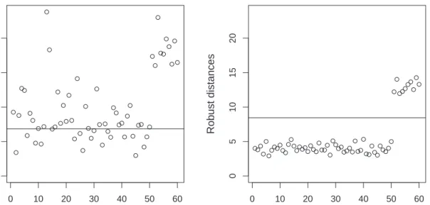
data set contains 10 gross errors, having indices 51 up to 60. Figure 2 plots the robust distances of the observations versus their index, once for the CR algorithm (left panel), and once for the GRID algorithm (right panel). The left panel of Figure 2 shows that the 10 gross-errors are correctly flagged as outliers, but there are also many good observations
having a large robust distance, some of them even a larger RDi than the true outliers.
Hence the CR algorithm suffers from the so-called swamping effect, meaning that good
observations are incorrectly flagged as outliers. This is due to the downward bias of the
estimated eigenvalues when using the CR algorithm, making the values in (11) too large.
On the other hand, the GRID algorithm clearly succeeds to pinpoint the 10 outliers, and separates well the outliers from the normal observations.
4
The GRID algorithm (GRID)
In this Section we propose the GRID algorithm. It is searching the space of all possible directions more thoroughly. A preliminary version of this algorithm was briefly discussed in [26], where it was applied to the robust continuum regression problem of [12]. As for the CR algorithm, we will first apply a pre-processing step by working with the scores
of the singular value decomposition (if p > n). In this section, we use the short hand
notation S(a) = S(xt
1a, . . . ,xtna), and our aim is to find the a maximizing S(a), under
the constraint that kak= 1. We will first explain in detail the algorithm for finding the
first optimal direction a1 in (1).
The basic idea behind the GRID algorithm is that the optimization problem is trivial
0 10 20 30 40 50 60 0 5 10 15 20 CR Index Robust distances 0 10 20 30 40 50 60 0 5 10 15 20 GRID Index Robust distances
Figure 2: Robust distances versus their indices for the artificial data set of Figure 1. Distances are once computed with the CR algorithm (left panel), and once with the GRID algorithm (right panel).
S((cos(θ),sin(θ))tover the interval [−π/2, π/2[.This can be done with an easy grid search,
i.e. we divide the interval in (Ng−1) equal parts, and evaluate the function at the grid
points (−1
2 + j
Ng)π, for j = 0, . . . , Ng−1. For Ng large enough, we will get close enough
to the solution. Note that a grid search is not asking for differentiability of the function to maximize, and can distinguish a global maximum from a local one.
In the general case, p > 2, the idea is to perform an iterative scheme of optimizations
in two-dimensional planes. Before starting, we relabel the indices of the columns of the
data matrix X in decreasing order of the value of Sj = S(x1j, . . . , xnj), for j = 1, . . . , p.
Hence, we may assume that S(e1) ≥ S(e2) ≥ . . . ≥ S(ep), where e1, . . . ,ep are the
canonical basis vectors.
1. Start with ˆa=e1.
Forj = 1, . . . , p
(a) Maximize the objective function in the plane spanned byej and ˆa, by a
grid search of the functionθ →S(cosθaˆ+ sinθej), where the angle θ is
restricted to the interval [−π/(2i);π/(2i)[.Denote θ0 the angle where the
maximum is attained over all grid points.
(b) Update ˆa←cosθ0aˆ+ sinθ0ej
So the first direction ˆawe are looking at is the one corresponding with the variable having
the largest dispersion. During one cycle, a sequence of grid searches over p−1 planes is
carried out; the jth grid search will update the jth coordinate of ˆa. When the second
cycle starts, it is assumed that the direction ˆa is already pointing in the good direction,
but still needs local improvement. Hence, the grid search will not search over the whole
plane, but only over the halfplane determined by the angles [−π/4, π/4[. After every
cycle, the search is limited to a more narrow interval of angles, but keeping the number
of grid pointsNg constant for every search. As such, the first few cycles will allow to find
the region of the search space where the maximum should be, and the subsequent cycles aim at further increasing the precision of the solution.
The subsequent optimal directions are found in a similar way. Once anak−1is obtained
(for k ≥ 2), a Householder transformation is applied to the data, corresponding to a
rotation of the data in such a way that ak−1 is transformed into the (k−1)th canonical
vector. Then the grid algorithm is applied again, but now only using the last (p−k+ 1)
coordinates of the data vectors. As such, a sequence of eigenvalues is obtained and, after inverting the Householder transformations, also a sequence of optimal directions. We refer to [5] for full details on this, and emphasize that due to the easy form of the Householder transformation and its inverse, the additional computational load is marginal.
Ifp > n, then the variables are exactly the scores on the principal components, and the algorithm is equivariant under orthogonal transformations. Furthermore, the algorithm
is completely deterministic, and easy to implement. Default choices are Ng = 10 and
Nc = 10, giving good results, also for noisy data sets containing many outliers. These
default choices are used throughout the paper.
5
Numerical Experiments
Simulation Experiment
of accuracy of the algorithm we take the value of ˆλ1, the maximum of the objective function
in (1). Since the aim of the algorithm is to attain the highest value in (1), better algorithms
provide higher values for ˆλ1. Also, the higher this value, the more informative, in terms
of higher variability, the obtained principal component is. Note that the highest possible
value, λ1 is in general not known, neither isa1. (An exception is the case where the scale
measure S equals the standard deviation, then λ1 and a1 are exactly computable from
an eigenvalue analysis of the sample covariance matrix). More generally, the precision of
the algorithm for finding the first k optimal directions will be measured by
Ik = k X j=1 ˆ λj, (12)
being the total variability accounted for by the firstkprincipal components. The efficiency
of the CR algorithm with respect to the GRID algorithm is then measured by
EFFk(CR;GRID) = ICR k IGRID k . (13)
It will turn out that throughout all numerical experiments we carried out, the above efficiency was nearly always below 100%.
Two situations are of special interest, namely the casen > pand the casen ≤p, where
after data compression the latter case corresponds to n=p. We take p= 50 throughout
this experiment, and set the sample sizen = 50 andn = 1000, respectively. Note that the
smaller sample size is the most important in chemometrical applications. Data are then
generated according to N(0, diag(λ1, . . . , λp)) with λj = 1/j2, yielding a fast decaying
scree plot. Since the algorithms are aimed at data containing outliers, further simulations are done for contaminated data: 80% of the observations of a simulated data set come from the same distribution as before, and the remaining 20% of observations are generated
due to N(0,10·diag(λp, . . . , λ1)). Hence the outlier generating distribution has exactly
the inverse order of principal components.
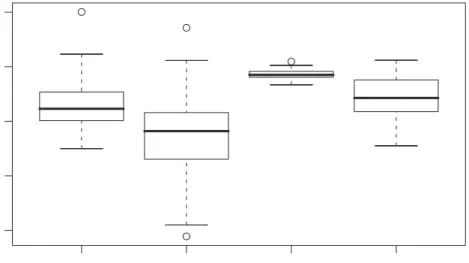
We generate 1000 different samples, and compute then the efficiency in (13), fork = 1.
Boxplots of these 1000 replicates are given in Figure 3, once for n = 50, and once for
n= 1000, for the data with and without contamination. As scale measure, the MAD was
taken here. It is seen from Figure 3 that the efficiencies remain below 100% in nearly
all cases, showing the superiority of the GRID algorithm over the CR algorithm. The difference becomes more pronounced for the lower sample size, where the median efficiency is about 85%. In presence of outliers, the relative performance of the GRID algorithm
n=50, clean n=50, contam. n=1000, clean n=1000, contam. 0.4 0.6 0.8 1.0 1.2 Efficiency
Figure 3: Boxplots of the efficiencies of the CR algorithm with respect to the GRID algorithm, for 1000 simulated samples of sizen = 50 andn = 1000, once without outliers (“clean”) and once with outliers (“contaminated”).
samples where the efficiency gain by the GRID algorithm is very considerable; for example,
for the contaminated case with n = 50, efficiencies of only 40% are observed in the
boxplots. We conclude from Figure3 that the GRID algorithm indeed yields much more
accurate approximations for the case n ≤p. On the other hand, for n = 1000> p = 50,
the CR algorithm performs reasonably well, and is not loosing much w.r.t. the GRID algorithm.
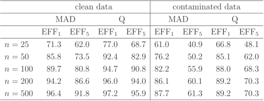
Table 1presents results for the same simulation setup, but with values for the sample
size n ranging from 25 to 500, and for both robust scale measures MAD (4), and once
for Q (5). Average efficiency measures are reported for k = 1 and k = 5. The standard
errors around these reported averages were always less than 1.4%.
The results in Table 1confirm the findings from the boxplots in Figure 3. The GRID
algorithm is much more accurate than the CR algorithm, in particular for the smaller sample sizes. This efficiency gain is even more important for contaminated data,
con-taining outliers. Moreover, the efficiencies EFF5 over the first 5 principal components
are consistently lower than the values EFF1, indicating that the inaccuracy of the CR
algorithm is cumulating over the additional components. It can also be seen that the efficiency gain when using MAD is more pronounced than for Q. This can be explained
Table 1: Average efficiencies of the CR- with respect to the GRID algorithm, forp= 50, several values ofn, for the MAD and Q, and for clean and contaminated simulated data.
clean data contaminated data
MAD Q MAD Q
EFF1 EFF5 EFF1 EFF5 EFF1 EFF5 EFF1 EFF5
n = 25 71.3 62.0 77.0 68.7 61.0 40.9 66.8 48.1
n = 50 85.8 73.5 92.4 82.9 76.2 50.2 85.1 62.0
n = 100 89.7 80.8 94.7 90.8 82.2 55.9 88.0 68.3
n = 200 94.2 86.6 96.0 94.0 86.1 60.1 89.2 70.3
n = 500 96.4 91.8 97.2 95.9 87.7 61.3 89.2 70.3
be much smoother than for MAD. Thus, a more precise algorithm like GRID will be able to identify local jumps close to the optimum whereas CR fails to find these peaks.
The computational effort of the GRID algorithm will be higher than that for the CR
algorithm. In fact, the GRID algorithm requires p×Ng ×Nc evaluations of the scale
measure, while the CR algorithm needs only n evaluations (for finding a single optimal
direction). Hence, to make the comparison more fair, we generated additional directions
to the considered search directions of (7) for the CR algorithm such that the computation
time becomes comparable (i.e. the number of evaluations ofS is the same). Interestingly,
the results of Table1remained almost identical. The only exception is the value of EFF5
forn= 25 and contaminated data, which increased from 40.9 to 51.2 when using the MAD,
and from 48.1 to 54.6 for the Q. Hence, unless the sample size is very small, generating
addition random directions is of little use. The reason is that the trial directions of (7)
are good candidate directions which cannot easily be improved by simply adding some
random directions to (7).
While the above simulation experiment indicates the superior performance of the GRID with respect to the CR algorithm, the efficiencies do not show how close the results
are to the true optimum of (3). Unfortunately, there is only one setting were this could
be verified, namely when the scale measure is the classical standard deviation. In this case, the maximal value of the objective function is given by the largest eigenvalue of the sample covariance matrix of the data. Thus, we repeated the same simulation exercise as above, comparing the GRID algorithm with the exact solution, and obtained that the computational efficiency of GRID with respect to the exact solution is almost 100% (re-sults available upon request). When the standard deviation serves as projection index, the GRID algorithm retrieves the exact solution upon rounding error.
2 4 6 8 10 12 14 0.03 0.04 0.05 0.06 0.07
Scale measure MAD
Number of components Cumulative eigenvalues GRID CR 2 4 6 8 10 12 14 0.03 0.04 0.05 0.06 0.07 Scale measure Q Number of components Cumulative eigenvalues GRID CR
Figure 4: Plot of the cumulated eigenvalues for the ‘Gas data’, as estimated by the algorithms GRID and CR, once using MAD and once for Q as projection index.
Real Data Examples
We compare the performance of the two algorithms also on two real data sets. The first
data set reports the NIR (near-infrared) spectra of n = 60 gasoline samples, measured
in 2nm intervals from 900nm to 1700nm (p = 401). It will be called the ‘Gas data’
being described in [27]. This is an example where the number of variables p is larger
than the number of observationsn. The second data set, called ‘Car data’, is available in
S-Plus ([28]), and illustrates a situation where the number of observations is larger than
the number of variables. In this example, p = 11 variables are evaluated from n = 111
different cars.
For both examples we considered the MAD and Q as robust scale measures. The
results are presented by plotting the cumulated eigenvalues defined by (8) with respect to
k, the number of principal components retained. Recall that (8) measures the variability
explained by the first k components. Figure 4 presents the results for the Gas data.
The plot suggest that after 6 to 8 components the extra gain in explained variability
by adding more components becomes much smaller, suggesting that k about 8 is a good
choice. The same trend as seen from the simulations studies is also visible here. The GRID algorithm yields much higher explained variabilities than the CR algorithm, resulting in more informative principal components.
2 4 6 8 10
250
300
350
400
Scale measure MAD
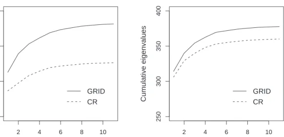
Number of components Cumulative eigenvalues GRID CR 2 4 6 8 10 250 300 350 400 Scale measure Q Number of components Cumulative eigenvalues GRID CR
Figure 5: Plot of the cumulated eigenvalues for the ‘Car data’, as estimated by the algorithms GRID and CR, once using MAD and once for Q as projection index.
can be made. Especially for the first few components the GRID algorithm shows much higher contributions to the explained variability than the CR algorithm. This is true for both scale measures, with the gain of the GRID algorithm being largest when the MAD is used.
6
Summary and Conclusions
Principal component analysis based on projection-pursuit (PP) is very attractive in many respects. By using different scale measures as Projection Index, different types of PCA are obtained. In particular, taking a robust scale measure like MAD or Q, yields a robustification of standard PCA. Moreover, it is possible to stop the computation of the principal components at any desired number of components, which is not the case for PCA based on a robust covariance matrix. Especially for high-dimensional data this is an important feature, since the computational effort can be reduced considerably by computing only the first few robust principal components.
We presented a new algorithm, called GRID, for computing the robust principal com-ponents and showed that it outperforms the currently available CR algorithm. In practi-cally all simulation situations and examples it turned out that the GRID algorithm leads to higher amounts of explained variability. The differences between the algorithms is
sub-stantial for small sample sizes withn < p, being the most pertinent case in chemometrical
applications. For a large sample sizenwith respect to the dimensionp, the CR algorithm
still performs quite well, as can be seen from the simulation results in Section 5. Note that the CR algorithm as proposed by [11] was not aimed at high dimensional applications. For n >> pwe still recommend this algorithm as a fast and reasonably accurate way to
find the robust principal components, but for p > n it should not be used. In particular,
we showed in Section 3 that the CR algorithm suffers from implosion breakdown in the latter case.
Note that the GRID algorithm works for any scale estimator, and no differentiability conditions are needed. Hence it is an “omnibus” algorithm that can serve to maximize any Projection Index. In this paper we focus on the widely used robust scale measures MAD and Q, and demonstrated that for both scale measures the algorithm GRID gives much better approximations to the eigenvalues than the CR algorithm. The choice of the scale estimator to be used must be based on statistical grounds, as discussed in [4]. The MAD is more robust, while the Q has a higher statistical efficiency.
In this paper we did not compare with other robust PCA approaches based on the Projection-Pursuit principle, since several papers have already been devoted to this (see Introduction). This paper is on a comparison of different algorithms for the same estima-tor, and not on comparing robust PCA estimators of different natures. If the aim of the principal component analysis method is to maximize explained variability, then the PP based approach is the natural estimator to use.
Both the GRID and the CR algorithm have been implemented in the freely available statistical software package R. They can be downloaded from (http://www.R-project.org)
as the library pcaPP, including as well further documentation for the user.
Acknowledgments
We would like to thank Heinrich Fritz from the Vienna University of Technology for translating the algorithms into C++ and for preparing the R library. We also thank the reviewers for their constructive comments.
References
[1] P.J. Huber, The Annals of Statistics, 13 (1985) 435-525.
[2] G. Li and Z. Chen, Journal of the American Statistical Association, 80 (1985)
759-766.
[3] Cui, H., He, X., and Ng. K.W, Biometrika, 90 (2003) 953-966.
[4] C. Croux and A. Ruiz-Gazen, Journal of Multivariate Analysis, 95 (2005) 206-226.
[5] M. Hubert, P.J. Rousseeuw, and S. Verboven (2002), Chemometrics and Intelligent
Laboratory Systems, 60 (2002), 101-111.
[6] I. Stanimirova, B. Walczak, D.L. Massart, and V. Simenov, Chemometrics and
In-telligent Laboratory Systems, 71 (2004) 83-95.
[7] M. Daszykowski, S. Serneels, K. Kaczmarek, P. Van Espen, C. Croux, and B.
Wal-czak, Chemometrics and Intelligent Laboratory Systems, to appear.
[8] M. Daszykowski, K. Kaczmarek, Y. Vander Heyden and B. Walczak, Chemometrics
and Intelligent Laboratory Systems (In Press), available online 28 August 2006.
[9] R.A. Johnson and D.W. Wichern, Applied Multivariate Statistical Analysis, 4th
edition, Prentice Hall, New York, 1998.
[10] Y. Xie, J. Wang, Y. Liang, L. Sun, X. Song, and R. Yu, J. Chemometrics 7 (1993)
527-541.
[11] C. Croux and A. Ruiz-Gazen, in A. Prat (Ed.), Compstat: Proceedings in
Compu-tational Statistics, Physica-Verlag, Heidelberg, 1996, pp. 211-216.
[12] S. Serneels, P.Filzmoser, C. Croux, and P.J. Van Espen, Chemometrics and Intelligent
Laboratory Systems, 76 (2005), 197-204.
[13] C. Croux and G. Haesbroeck, Biometrika, 87 (2000) 603-618.
[14] R.A. Maronna, Technometrics, 47 (2005) 264-273.
[15] M. Hubert, P.J. Rousseeuw, and K. Vanden Branden, Technometrics, 47 (2005)
64-79.
[16] P.J. Rousseeuw and C. Croux, Journal of the American Statistical Association, 88
[17] A. Weber, ¨Uber den Standort der Industrien, T¨ubingen. English translation by C. Friedrich (1929): Alfred Weber’s theory of location of industries. University of Chicago Press, 1909.
[18] O. H¨ossjer and C. Croux, Nonparametric Statistics 4 (1995) 293-308.
[19] U. Gather, T. Hilker, and C. Becker, in L.T. Fernholz, S. Morgenthaler, and W.
Stahel (Eds.), Statistics in Genetics and in the Environmental Sciences, Birkhauser, Basel, 2001, pp. 147-157.
[20] G. Boente, A.M. Pires, and I.M. Rodrigues, Biometrika 89 (2002) 861-875.
[21] P. Filzmoser, Environmetrics 10 (1999) 363-375.
[22] I. Stanimirova, M. Daszykowski, E. Van Gyseghem, F.F. Bensaid, M. Lees, J,
Smeyers-Verbeke, D.L. Massart, and Y. Vander Heyden, Analytica Chimica Acta, 552 (2005) 1-12.
[23] D.L. Donoho and P.J. Huber, in P.J. Bickel, K.A. Doksum, and J.L. Hodges (Eds.),
A Festschrift for Erich L. Lehmann, Wadsworth, Belmont, CA, 1983, pp. 157-184.
[24] P.J. Rousseeuw and A.M. Leroy, Robust Regression and Outlier Detection. John
Wiley, New York, 1987.
[25] C. Croux and P.J. Rousseeuw, Communications in Statistics, Theory and Methods,
21 (1992) 1935-1951.
[26] P. Filzmoser, S. Serneels, C. Croux, and P.J. Van Espen, in M. Spiliopoulou, R.
Kruse, C. Borgelt, A. N¨urnberger, and W. Gaul (Eds.), From Data and Information Analysis to Knowledge Engineering, Springer, Berlin Heidelberg, 2006, pp. 270-277.
[27] J.H. Kalivas, Chemometrics and Intelligent Laboratory Systems, 37 (1997) 255-259.